
A Sequential Approach for Aerodynamic Shape Optimization with Topology Optimization of Airfoils †


1
Instituto Superior Técnico, Universidade de Lisboa, Av. Rovisco Pais, 1049-001 Lisboa, Portugal
2
IDMEC, Instituto Superior Técnico, Universidade de Lisboa, Av. Rovisco Pais, 1049-001 Lisboa, Portugal
3
DAEP, ISAE-SUPAERO, Université de Toulouse, 10 av. Edouard Belin, BP 54032, 31055 Toulouse, France
*
Author to whom correspondence should be addressed.
†
This paper is an extended version of our paper published in 5th International Conference on Numerical and Symbolic Computation Developments and Applications (SYMCOMP 2021).
Math. Comput. Appl. 2021, 26(2), 34; https://doi.org/10.3390/mca26020034
Submission received: 11 March 2021
/
Revised: 16 April 2021
/
Accepted: 17 April 2021
/
Published: 20 April 2021
(This article belongs to the Special Issue Numerical and Symbolic Computation: Developments and Applications 2021)
Abstract
:The objective of this work is to study the coupling of two efficient optimization techniques, Aerodynamic Shape Optimization (ASO) and Topology Optimization (TO), in 2D airfoils. To achieve such goal two open-source codes, SU2 and Calculix, are employed for ASO and TO, respectively, using the Sequential Least SQuares Programming (SLSQP) and the Bi-directional Evolutionary Structural Optimization (BESO) algorithms; the latter is well-known for allowing the addition of material in the TO which constitutes, as far as our knowledge, a novelty for this kind of application. These codes are linked by means of a script capable of reading the geometry and pressure distribution obtained from the ASO and defining the boundary conditions to be applied in the TO. The Free-Form Deformation technique is chosen for the definition of the design variables to be used in the ASO, while the densities of the inner elements are defined as design variables of the TO. As a test case, a widely used benchmark transonic airfoil, the RAE2822, is chosen here with an internal geometric constraint to simulate the wing-box of a transonic wing. First, the two optimization procedures are tested separately to gain insight and then are run in a sequential way for two test cases with available experimental data: (i) Mach 0.729 at ; and (ii) Mach 0.730 at . In the ASO problem, the lift is fixed and the drag is minimized; while in the TO problem, compliance minimization is set as the objective for a prescribed volume fraction. Improvements in both aerodynamic and structural performance are found, as expected: the ASO reduced the total pressure on the airfoil surface in order to minimize drag, which resulted in lower stress values experienced by the structure.
1. Introduction
The usage of numerical optimization algorithms has allowed for lighter and more aerodynamically efficient wing designs. These algorithms include, among others, Aerodynamic Shape Optimization (ASO) and Topology Optimization (TO). In the former, a given shape, for example a wing or an airfoil, after being adequately parameterized is optimized for a specific aerodynamic goal, such as lift-to-drag ratio maximization or drag minimization, while fulfilling a prescribed set of constraints. The latter consists in finding an internal structure that minimizes its compliance in a given solid domain for a known set of boundary conditions. ASO [1] and TO [2] have been applied in both academic and industrial applications related to aeronautics, including wings and airfoils.
TO is a useful computational tool that can be used to reach lighter wing structures and so it has been applied to different aircraft types such as transport, unmanned aerial vehicles and even micro air vehicles in recent decades. Maute and Allen [3] developed a framework to optimize the topology of a wing structure considering Fluid-Structure Interaction (FSI). Krog et al. [4] in a joint effort between Airbus and Altair tested different topology optimization strategies considering 10 load cases to optimize a wing-box rib. Gomes and Suleman [5] used TO for the design of a wing-box such that the aileron reversal speed is maximized. Stanford and Ifju [6] used aeroelastic TO to design the membrane structure of a micro air vehicle’s wing, considering different objective functions including lift-to-drag ratio maximization. In [7], the authors tested their TO methodology on the internal structure of a tapered and swept wing-box, formed by a constant symmetrical airfoil, subjected to a pressure load. They observed an asymmetrical structure, formed to withstand the also asymmetrical span-wise pressure load, which presents more material near the root to support the bending and cross trusses to withstand shear. In [8], the internal structure of a unmanned aerial vehicle’s wing is optimized recurring to TO considering aerodynamic loads. Dunning et al. [9] optimized the wing of the Common Research Model (CRM) considering the trimmed lift. Félix et al. [10] considered the wing’s self-weight, besides an aerodynamic load, to design it topologically. Capasso et al. [11] employed TO to design a morphing structure made of a hyperelastic material.
ASO of airfoils and wings can be conducted by means of a gradient-based optimization algorithm or a gradient-free one. The former is more common than the latter and it is particularly efficient when gradients are computed by means of the adjoint method [12] to explore high-dimensional design spaces and find local minima [13]; however, global search gradient-free algorithms (such as genetic algorithms) might be more adequate to find a global minimum. Nemec et al. [14] performed ASO of the RAE2822 airfoil for two objectives and multiple flow conditions, using a gradient-based algorithm where the sensitivities are computed by means of the adjoint method. The results obtained compared well with those reached with a genetic algorithm. Later, Zingg et al. [15] compare these two optimization approaches for ASO of airfoils, reaching the conclusion that despite both reached the same solution, the latter one takes 5 to 200 times longer than the former. Martins and his coworkers have been conducting ASO using gradient-based optimizations for several wing applications, spanning from conventional aircraft configurations [16] to unconventional solutions (e.g., camber morphing [17]) and designs (the blended-wing-body [18] and the strut-braced wing [19]) with the aim of improving performance. Several parameterization techniques are compared for ASO of airfoils in [20], including Free-Form Deformation (FFD), non-uniform rational B-Splines (NURBS), Class Function/Shape Function Transformations (CST) and Hicks-Henne. The authors noticed that 20 to 25 design variables are required to fully cover the design space. De Gaspari and Ricci [21] developed a framework to design camber morphing solutions which consists of two steps: (i) first a gradient-based optimization of the aerodynamic shape of the airfoil is done for a given objective; and (ii) then an internal truss-like structure is optimized such that is able to achieve the desired morphing shape, using a genetic algorithm. Antunes and Azevedo conducted their ASO studies using genetic algorithms [22]. Surrogate models based on machine learning have also been studied for ASO of airfoils using both gradient-free [23,24] and gradient-based [25] algorithms. With these surrogate models the computational burden of ASO can be relieved at a cost of generating large databases. The computational cost of the latter can overpass the former if only a reduced number of optimization iterations are needed as noted by Bouhlel et al. [25].
Despite these optimization algorithms having been employed in several wing and airfoil applications, their combined application is much less common in the literature. ASO is normally done before the TO as in [26], although there are some papers where two optimizations process are carried out simultaneous for performance [27] or aeroelastic applications [28]. Maute and Reich [26] developed a sequential framework to design morphing structures based firstly on ASO and secondly on TO. James et al. [27] coupled both optimization processes in their Multidisciplinary Design Optimization (MDO) framework and compared it with the sequential approach for the design of the Common Research Model (CRM) wing. They noticed that their coupled approach was able to achieve a wing model with 18% less drag than with the sequential approach. Gomes and Palacios [28] applied a fully-coupled aerodynamic and stiffness-based TO methodology for designing a compliant airfoil using FSI. Their methodology consists in two sequential steps: (i) firstly, the airfoil shape is optimized for a given aerodynamic-related objective and a set of constraints considering both ASO and TO; (ii) followed by an inverse design where the internal structure is optimized for a mass minimization objective.
These works [26,27,28] use the Solid Isotropic Material with Penalization (SIMP) model [29] to parameterize the structural domain, while in the present work the Bidirectional Evolutionary Structural Optimization (BESO) model [30] is used. BESO has the main advantage of being able to both remove and add material, and it has been applied to solve both academic and industrial problems [31]. This model has been applied to the structural design of a hypersonic wing considering aerothermoelasticity by Munk et al. [32]. For the present work, the authors developed a sequential framework to optimize airfoils considering both ASO and TO. To the authors’ best knowledge TO with BESO has not been coupled with ASO for airfoil applications.
This paper is organized as follows: first a literature review is provided in Section 1; followed by the theoretical background required to conduct aerodynamic shape optimization and topology optimization of airfoils in Section 2; then the methodology employed in this work is presented in Section 3; followed by the obtained results in Section 4; and ending with the concluding remarks drawn from this study in Section 5.
2. Background
This section presents a brief introduction to the theory behind the methods used in the aerodynamic shape optimization and topology optimization parts of this work.
2.1. Aerodynamic Shape Optimization
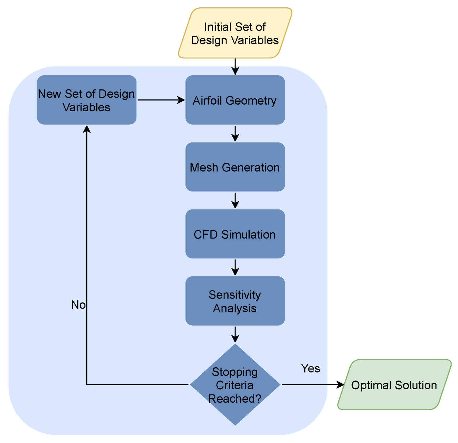
Aerodynamic shape optimization is the process of obtaining the set of design variables that produce the best (minimum) value of a single or a set of objective functions , while coping with a set of inequality and equality constraints. The objective function is dependent on both the design variables and the solution of some equations (represented by the vector of conservative variables ) that can be expressed as the residual . A general view of the problem can be defined as
Typical objective functions are the lift or drag produced by an airfoil (or their ratio), and the design variables are parameters that define the shape of the airfoil by means of a particular parameterization. A flowchart depicting the Aerodynamic Shape Optimization process followed is provided in Figure 1.
2.1.1. Flow Governing Equations
In this work, the flow is modeled by the Reynolds Averaged Navier–Stokes (RANS) equations, using the turbulent model provided by Spalart and Allmaras [33]. The final formulation for the RANS model can be described in a differential form [34] as
where is the domain, is the vector of conservative variables defined as , being the density, the velocity and E the total energy. is the numerical residual, the source terms and the respective convective and viscous fluxes, defined as
and
with T being the temperature obtained from the ideal gas equation of state, p the static pressure, the thermal conductivity and the viscous stress tensor. Further information on the details of the equations can be found in [34].
2.1.2. Adjoint-Based Gradient Computation
The adjoint method provides an efficient way of computing the gradients of a set of objective functions with respect to a set of design parameters with a computational cost that is nearly independent of the number of design parameters. It is particularly advantageous in aerodynamic shape optimization problems where the number of objective functions (and constraints) is usually much smaller than the number of design parameters. The adjoint of the flow governing equations can be expressed as
where is the adjoint vector, or solution, which can be used to compute the total gradient of f with respect to as
The system of equations in (5) only has to be solved once for each objective function f (and for each constraint). The choice of design variables is only limited to the possibility of being able to define the objective function, constrains and residual as a function of those same variables. Typically, in ASO, the computational mesh coordinates are used, and the sensitivity of the function of interest to a more meaningful design parameter can be obtained using the chain-rule as
The last term of the previous equation will depend not only on the geometry definition approach but also on the mesh generation/deformation technique that is used.
2.1.3. Parametrization Technique: Free-Form Deformation
In this work, the Free-Form Deformation (FFD) methodology is used. Developed by Sederberg [35] to model solids, it has its recognition not only due to its versatility but also since it does not manipulate directly the geometry of the object, in opposition to other parametrization techniques, but rather the lattice of a certain region in the domain where the object is embedded. For two-dimensional cases the region looks like a rectangle and like a parallelpiped for 3D cases. A set of control points are defined on the surface of the enclosing region. Their number depends on the order of the chosen Bernstein polynomials. The points inside this region can then be parameterized as a FFD function
where are the degrees of the FFD function, are the parametric coordinates of and , and are the Bernstein polymonials. By modifying the control points defined along the boundaries of the parallelpiped region, the points inside (and thus, the geometry they define) inherit a smooth deformation.
2.2. Topology Optimization
Topology optimization is a numerical method used to determine the best material distribution for a given set of boundary conditions. Different algorithms can be used for this task, such as the SIMP or BESO. The latter is used for this work.
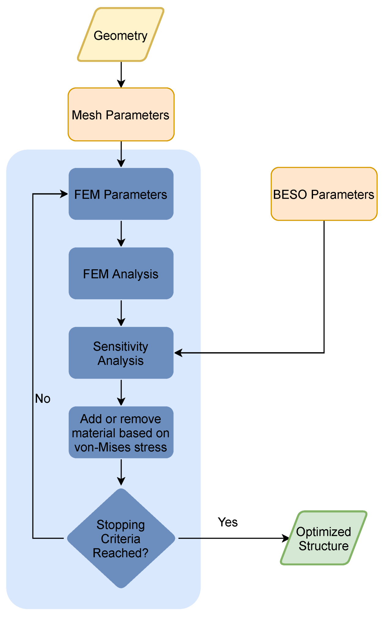
The BESO algorithm removes material from the low-stressed areas of a domain which is understood to be inefficient and adds material where it is strictly necessary to provide a higher stiffness to the structure. A ’hard-kill’ method is used, which uses two ratios: (i) a rejection ratio to mark as removable the material at elements with values lower than this parameter; and (ii) an addition ratio to identify elements which are assigned material for value higher than this ratio. The rejection criteria uses the von Mises stress of a cell, , and compares it with a threshold, , which could be a maximum or a prescribed value, thus:
The followed procedure aims at finding the stiffest geometry for a given volume, one of the most common goals in topology optimization. The objective is thus to minimize the strain energy (and consequently the compliance) for a given volume fraction, by attributing material or void to each element of a previously defined mesh of the structure. A standard formulation of this problem is as follows:
In the above equation: C is the mean compliance of the structure; u and f are the displacement and load vectors, respectively; denotes the target volume fraction; is the volume of each element; N is the total amount of elements, which corresponds to the number of design variables; is the binary description of the presence of mass, being 0 a void and an 1 a filled state; and K is the stiffness matrix of the structure.
A general view of the algorithm followed is depicted in Figure 2.
Regarding the solid mechanics theory behind the case of study, the airfoil structure is considered to behave inside the elastic region of the material, specifically within the linear region. Therefore, the Hooke’s law is valid, which implies a proportional relation between the stresses and the correspondent strains by means of the constitutive matrix D:
For isotropic materials, the constitutive matrix requires only the Young’s modulus E and the Poison ratio . The strains relate with displacements by means of the strain-displacement matrix B as follows:
3. Methodology
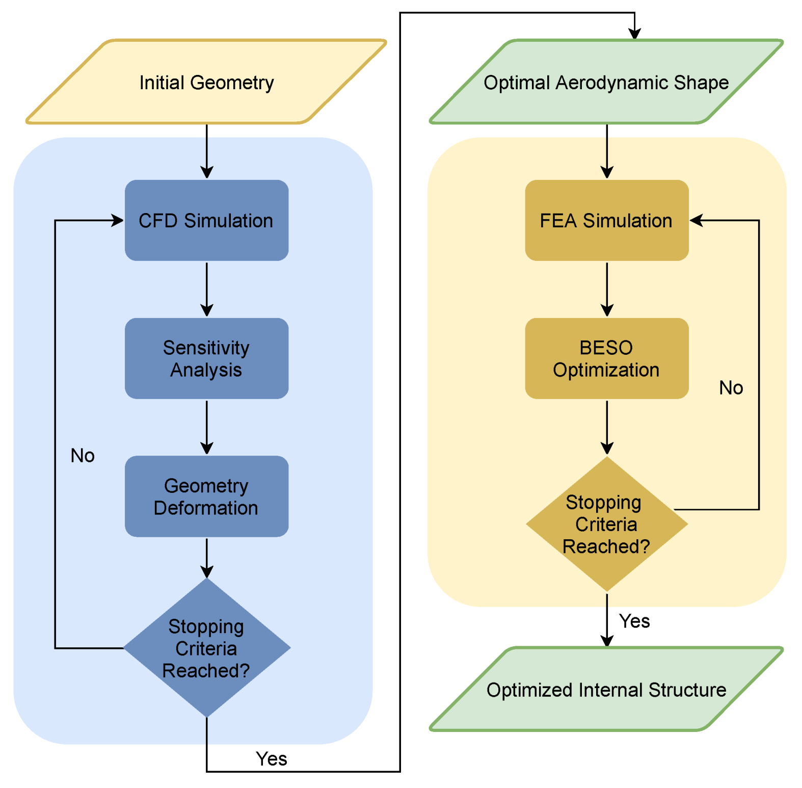
In this work, a sequential optimization approach is followed, where for a given airfoil: (i) first its shape is optimized considering only aerodynamics; and (ii) then its internal structure is topologically optimized for the resulting aerodynamic load. This process is depicted in Figure 3 and its steps are thoroughly discussed in this section.
The RAE2822 transonic airfoil is chosen for this work since it is widely used in the literature [14,20], due to the availability of experimental data [36] to validate the obtained Computational Fluid Dynamics (CFD) results. It was designed specifically for transonic regimes where a shock-wave is present, specially at the Reynolds number for which the simulations are established, i.e., . Given the fact that experimental data is available in [36] the following conditions of Reynolds number, Re, Mach number, M and angle of attack, , are considered in this work: (1) , and and (2) , and .
3.1. Aerodynamic Shape Optimization
The flow governing equations of the aerodynamic problem are solved using the finite-volume solver SU [34]. Widely used in aerodynamic shape optimization problems, it is coupled with the SciPy library for gradient-based optimization, with the gradients being computed using the adjoint method. The Sequential Least Squares Programming (SLSQP) is used as the optimization algorithm.
3.1.1. Mesh Definition
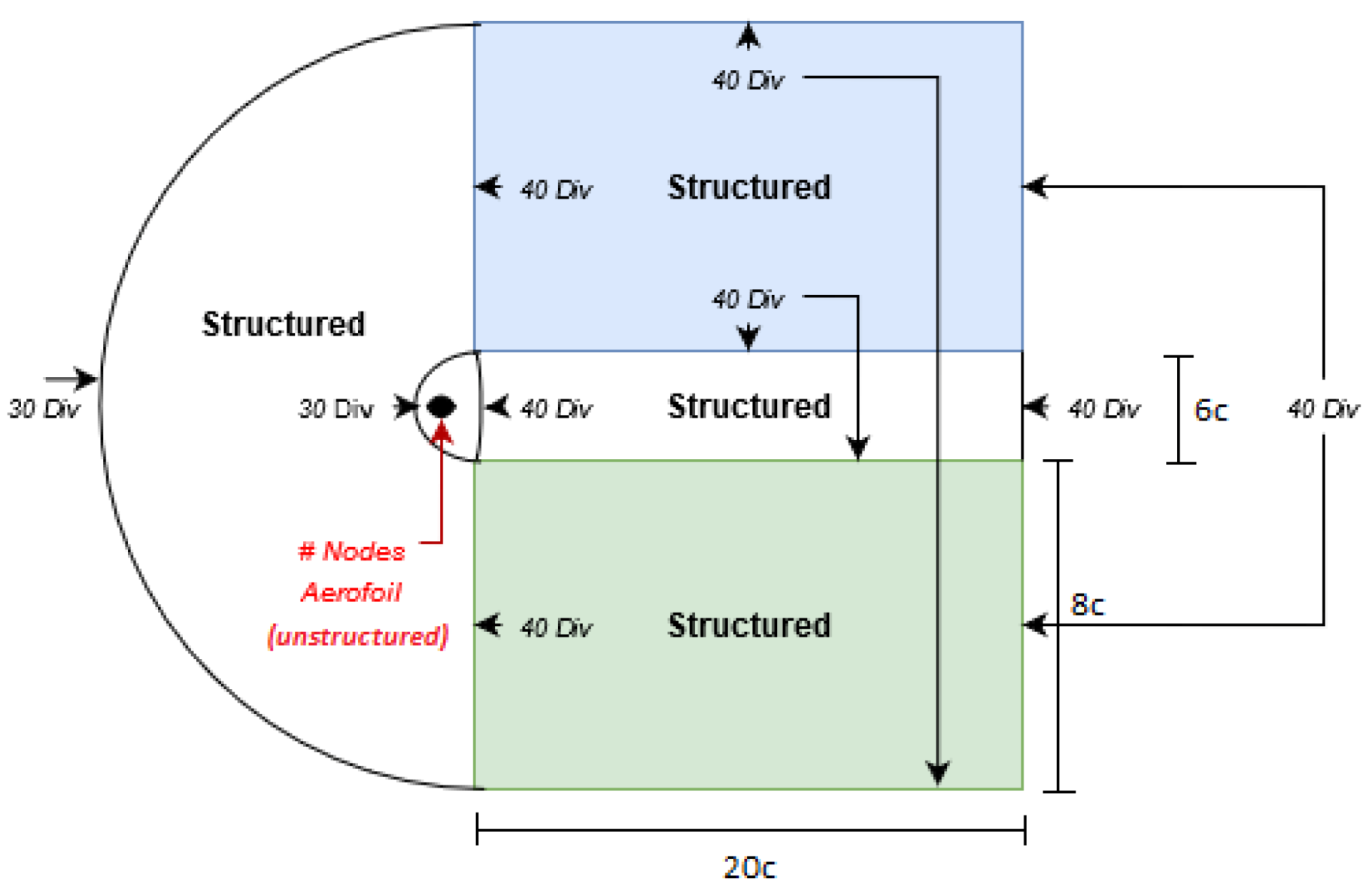
The computational mesh for the aerodynamics simulation is a C-type mesh, as illustrated in Figure 4, generated using Gmsh while taking the following considerations into account, to obtain good mesh quality: (i) the constraints are applied at the domain’s boundaries such that they do not have a noticeable influence on the results [37]; (ii) mesh quality parameters are evaluated (e.g., element’s orthogonality and flow alignment); (iii) the magnitude of the parameter is tracked to adequately represent the flow in the boundary layer; and (iv) a far-field boundary condition is set.
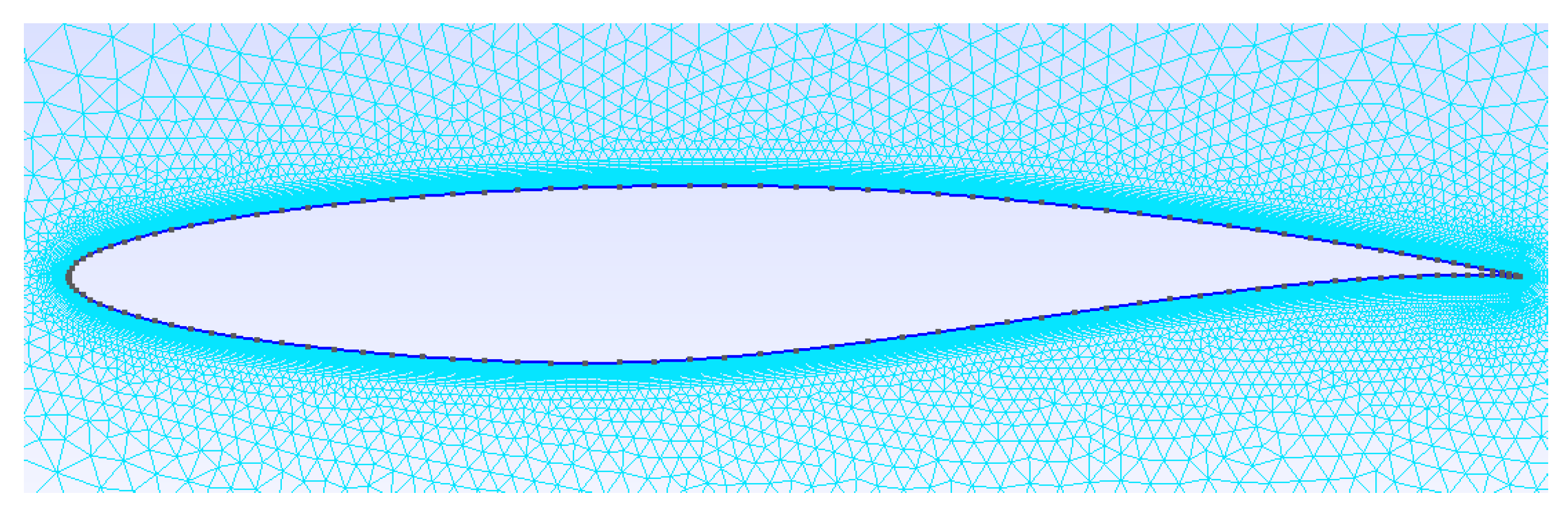
Moreover, a mesh refinement is applied at the airfoil geometry to adequately represent the boundary layer development, converting the grid into a structured distribution with several layers surrounding the airfoil (see Figure 5) aiming at a wall-grid spacing of c, where c is the airfoil chord.
Following a mesh convergence study, presented in Table 1, a mesh with a total number of 53,492 elements was selected, providing a trade-off between results accuracy and computational requirements. Though aware that a finer mesh would provide more accurate results, the limited computational resources available together with a relative difference of only 5% in the drag coefficient (lift coefficient was already converged) led to the selection of the medium mesh in the ASO. In what concerns the lift and drag coefficients, listed in Table 2, the results of the medium mesh also compare well with the experimental data. Relative differences of 3.7% and 8.2% are obtained for the lift and drag coefficients, respectively, which is deemed acceptable for the purpose of this work.
3.1.2. Optimization Problem
After defining a suitable mesh for the fluid domain, the optimization problem can be defined in the SU environment by setting the objective function, constraints and design variables.
To explore the potential of ASO, two case studies previously mentioned are optimized. Both aim at drag minimization for a given lift coefficient, which are set as objective function and constraint, respectively. Table 3 presents the initial values of and for the two cases.
The design variables are defined based on the FFD method, which is used to parametrize the airfoil. The airfoil is enveloped in a box, as illustrated in Figure 7, that can be deformed by a given set of control points, acting as design variables. This box is designed such that it is close but does not intersect the airfoil surface. Since in a wing model the airfoil would have a wing-box crossing it, no design variables are added to the problem in the region of the wing box (delimited in Figure 7 in red) to prevent the surface deformation in that region. The hypothetical wing-box is defined between 25% and 75% of the chord. In the end, a total of 30 design variables, as identified in Figure 7, is used in the optimization process.
3.2. Topology Optimization
The topology optimization problem is solved using the BESO algorithm as described in [38] and available in [39]. The structural analysis is performed with the Finite Element Model (FEM) open-source solver Calculix.
3.2.1. Finite Element Model Definition
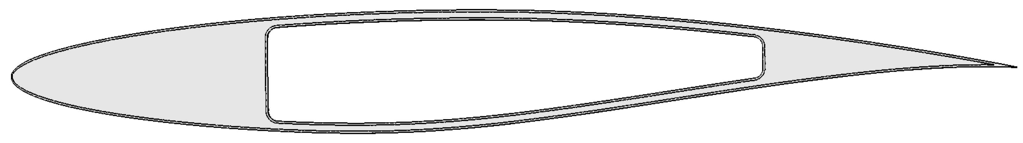
Once the aerodynamic optimization results are obtained, the pressure distribution along the airfoil’s surface is set as an input for the Finite Element Model (FEM) to be built. The structural domain, marked in gray in Figure 8, is discretized in triangular elements and is delimited externally (airfoil’s surface) and internally (wing-box) by skins of constant thickness 0.002c and 0.008c, respectively. An aluminum with the following properties is considered for this work: Young’s modulus GPa; Poisson ratio ; and material density kg/m.
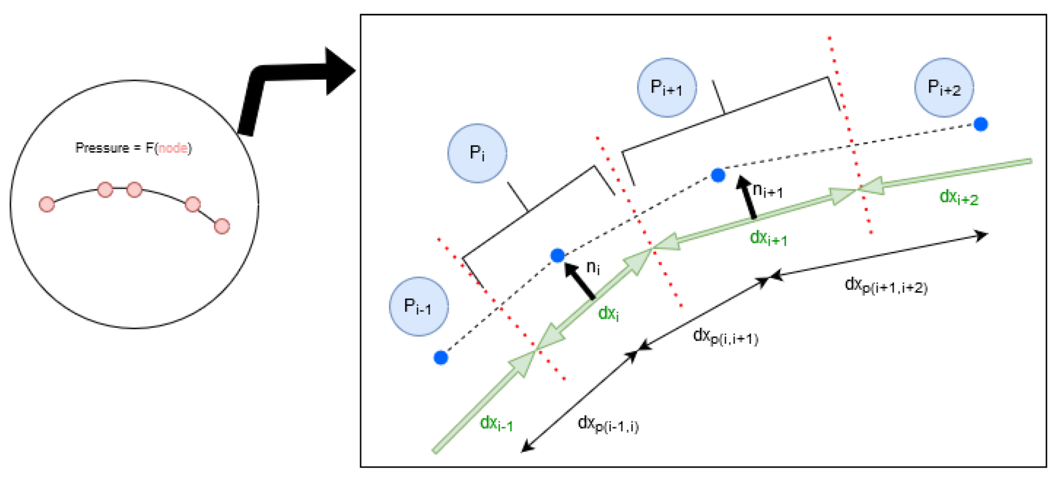
The pressure distribution obtained from the CFD simulations is applied on the airfoil’s skin as a load, after preprocessing it. As the pressure is discretized in the nodes, the loads should follow the same behavior. Therefore, the load should be applied at the node where its correspondent pressure value is obtained. To do so, the second space variable is defined using the initial geometry lines between nodes. By coupling the halves of the previous segment and the following one coming from the primary geometry, a balanced and accurate representation is achieved. Furthermore, the pressure value is not applied then at the node but at the new formed line following the direction of its normal vector. Then, the force direction depends on the magnitude of the pressure, being towards the inner structure when it is positive and outwards when it is negative. An illustration of this process is given in Figure 9.
In Figure 9, the initial nodes are marked in blue and the geometry is represented by black dashed lines. Then, the distance between nodes is also provided with the variable . Before the FEM analysis, the initial segments are divided in their mid-point, as seen in the red dotted lines; subsequently new segments are formed which connect the mid-nodes and save the information in the variable, which also has its own normal vector . Therefore, and shown by the brackets, the pressure value from the specific aerodynamic node is applied along that surface defined by .
As a boundary condition for the FEM analysis, the displacements and rotations in the wing-box are set to zero, thus constraining the airfoil on that internal surface.
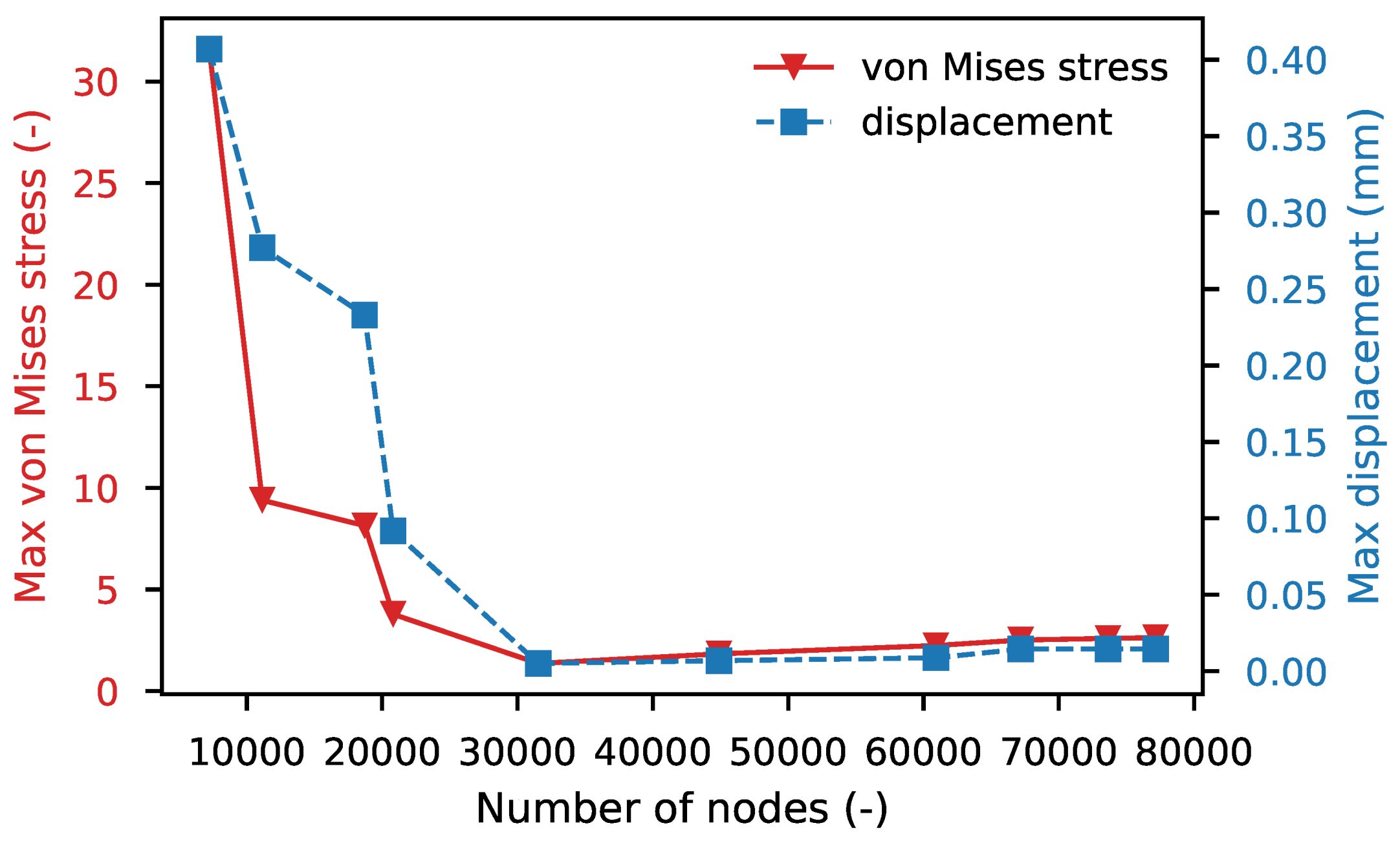
A mesh convergence study to evaluate its impact on the results is then carried out for the gray domain in Figure 8. Different meshes are generated for this task and their results are shown in Figure 10 for the maximum values of von Mises stress and displacement. Even though convergence is reached for about 30,000 nodes, the largest mesh (77,144 nodes) is chosen due to the reasonable computational cost and potential to better explore the design space in the TO problem.
3.2.2. Optimization Problem Definition
The objective function for the TO problem is set to minimize the compliance-to-weight ratio (i.e., to maximize the stiffness-to-weight ratio) for a given volume fraction; the latter is set as a problem constraint. The design variables are the presence or absence of material in the previously defined design domain.
To avoid instabilities such as the checkerboard pattern [40], a filter as described in [30] is employed for this work. Some parameters are then defined to improve the results, such as the filter radius and the mass addition and removal rates. These parameters are set after performing some studies, which led to the following choices: filter radius of 0.01c, which represents 8 to 10 times the mesh element size; mass addition and removal ratios of 1% and 4%, respectively, which means that at each iteration, the solver can add up to 1% material or remove up to 4%.
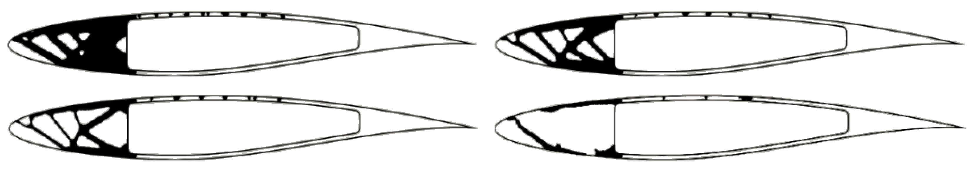
The influence of the prescribed volume on the structural topology is also evaluated. Figure 11 shows the layouts obtained for 50%, 35%, 25% and 10%. Despite the failure index criteria being lower than 1 for the 10% structural layout, the authors opted to use the 25% volume fraction for the results section.
4. Results
This section is divided intro three subsections. The first presents the results of the aerodynamic optimization of the profile, aiming at the drag minimization. In the second subsection, the results of the structural analysis of a filled aerodynamically optimized airfoils (with the exception of the wing box) are presented and discussed. Lastly, the third section presents the results of the topological optimization of the optimal airfoils of the two study cases.
4.1. Aerodynamic Optimization
As previously stated, two case studies are aerodynamically optimized by fixing the lift coefficient and minimizing the drag. Furthermore, the wing-box area of the airfoil is also set as fixed (as illustrated in Figure 7), thus any shape modifications only appear at the leading and trailing edges.
4.1.1. Case 1
The optimized solution for the first case study involves small deformations which, despite small, reduced the drag coefficient by 13.9% as it can be seen from Table 4.
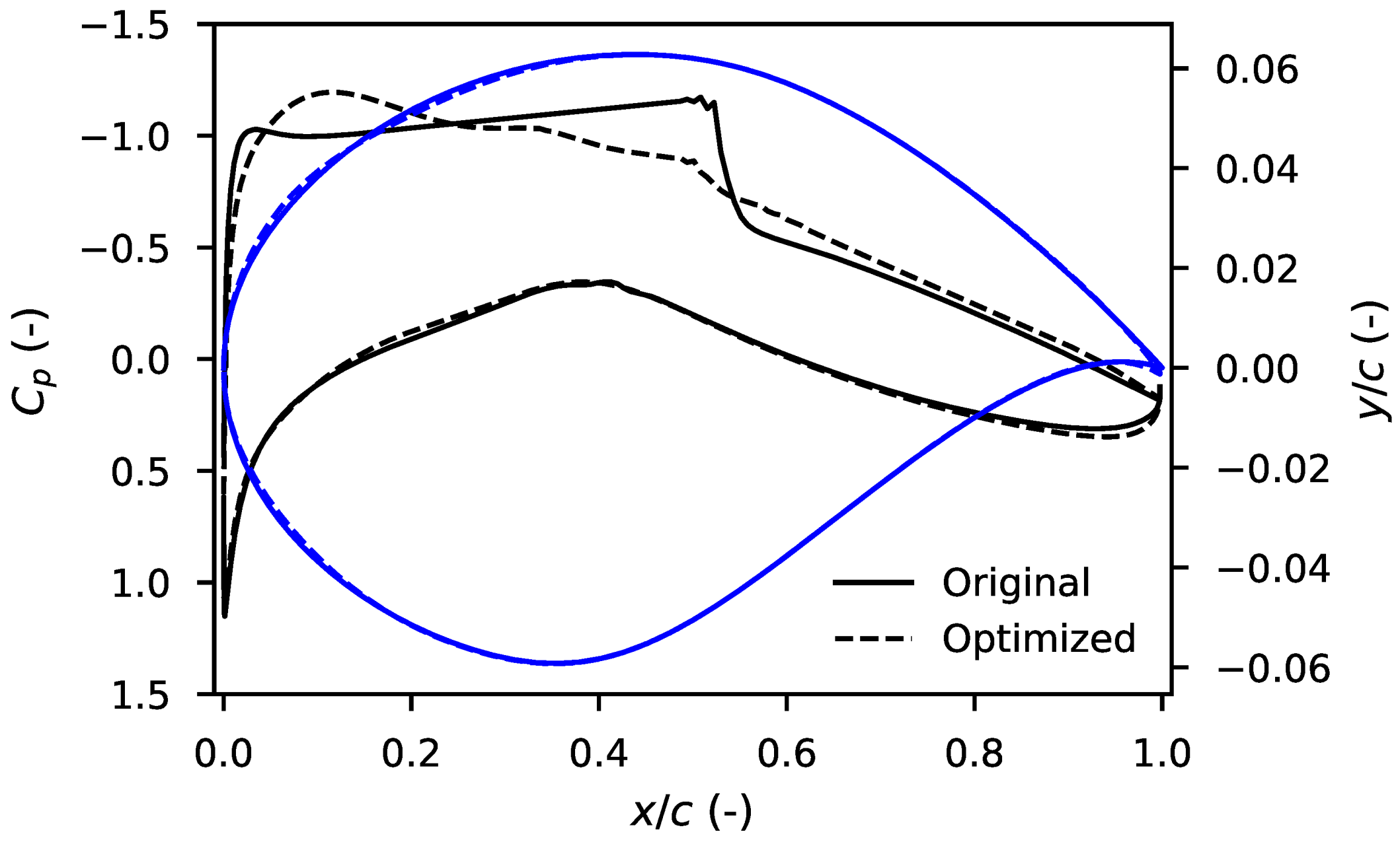
When analyzing the pressure distribution shown in Figure 12, it is possible to observe that even for small modifications in shape the pressure distribution substantially changes. The magnitude of the highest shape deformation is , thus highlighting the impact that sensitivity analysis has on the optimized result. Note that in order to reduce the drag while constraining the lift, the solver tries to increase the curvature near the leading edge in order to absorb some of the kinetic energy near the shock-wave formation.
4.1.2. Case 2
For the second case study, an even higher drag reduction (29.04%) than in the first case is reached, as shown in Table 5. Despite the geometric changes in the leading edge being more visible for this case, a similar approach as before is followed.
Regarding the pressure coefficient distribution along the airfoil, Figure 13, there is a higher peak of suction closer to the leading edge than in Figure 12. As well as in the previous case, the greater magnitude of the modifications of the geometry is in the order of (if the chord was defined as 1 m, the deformation would be 5 mm), thus it is not easily noticed.
4.2. Structural Results
For the two aerodynamically optimized airfoils, a completely-filled airfoil structure is studied in terms of the displacements and stresses caused by the pressure load. In this section, visual and numerical comparisons are provided for the two case studies.
When aerodynamically optimizing the airfoil’s shape, the stress and displacements distributions inside the airfoil change completely for both case studies, not only in magnitude, as it can be seen in Table 6, but also in its location. The aerodynamic load is reduced for the optimized airfoils since drag is minimized for the same lift coefficient. As a consequence, the stress and displacement values are also lower for the optimized airfoil’s structure.
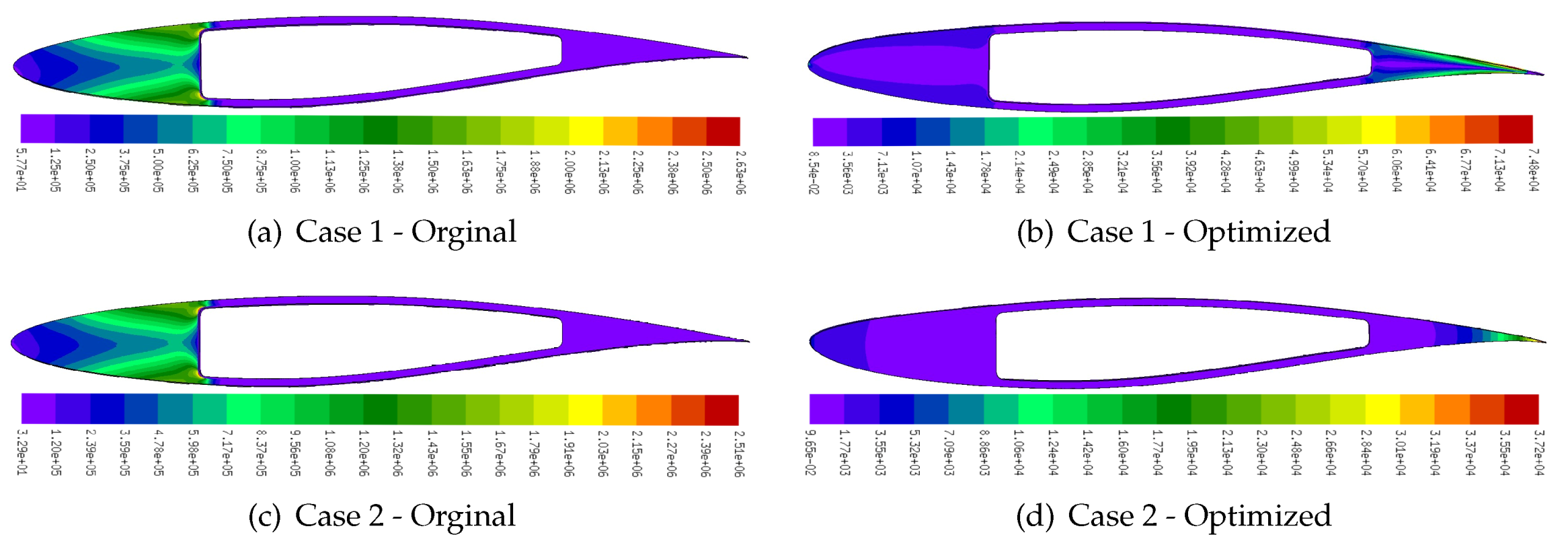
In Figure 14, the von Mises stress distribution is compared for the two case studies, considering the original and aerodynamically optimized airfoils. The displacement distribution is not plotted since its magnitude is very small when compared to the chord.
Regarding the first case, the maximum von Stress value has substantially decreased in 97%, from 2.63 MPa to 74.8 kPa, while the stress distribution has moved towards the trailing edge, where it has the lowest material density. For the second case study, the new stress distribution represents only 1.48% of the loading state for case 1, reaching a maximum value of 37.2 KPa. It is worth noting how very small changes to the airfoil surface can influence so considerably the stress distribution.
4.3. Aerodynamic and Structural Optimizations
As previously mentioned and illustrated in Figure 3, a sequential approach is followed in this work since it can provide useful insights on the design of aerostructurally optimized airfoils, even though the authors recognize that a fully coupled approach would have the potential to reach further optimized solutions. Here, an aerodynamic shape optimization is first conducted to the airfoil, followed by a topology optimization to its structure.
4.3.1. Case 1
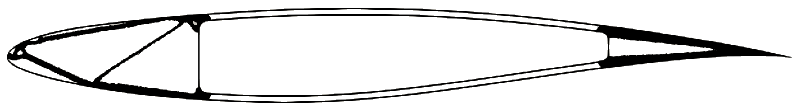
The topologically optimized structure is depicted in Figure 15, considering a volume fraction of 25%.
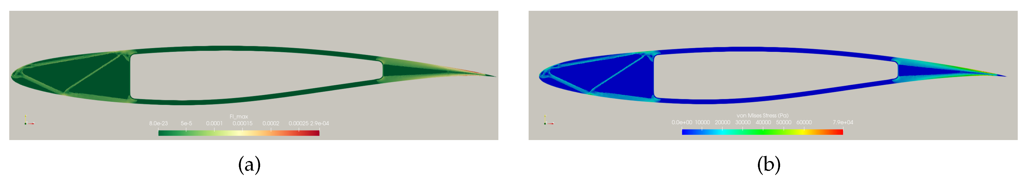
It is worth pointing out how the Failure Index (FI) of Figure 16a is two orders of magnitude lower than in the original airfoil suggesting that, from a first case, the structure should perfectly withstand the loading state. In terms of stresses (Figure 16b), the structure finds itself in a more relaxed situation, because the pressure loads are softened when the airfoil is aerodynamically optimized and are also absorbed in the leading edge region due to the appearance of new material. Apart from this latest statement, note how the inner stresses have a higher value than in the completely material-filled airfoil shown in Figure 14b (but in the same magnitude range), which is expected since the main purpose of the topology optimization is to redistribute the loads towards specific regions of the geometry while removing the unnecessary ones.
4.3.2. Case 2
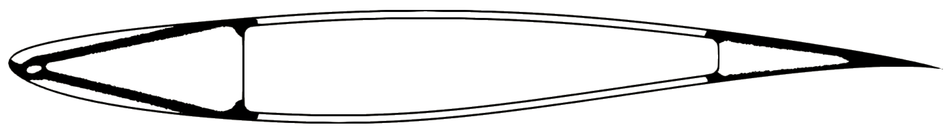
The second case study resulted in a slightly different topologically optimized structure depicted in Figure 17, as expected since the load is also slightly different.
A similar comment regarding the failure index and stresses distribution can be made for this second case study. It is worth noting that these two parameters are now slightly smaller as can be seen from Figure 18.
5. Concluding Remarks
This research aimed at coupling both aerodynamic and structural designs of airfoils using efficient optimization tools such as aerodynamic shape optimization and topology optimization. Firstly, based on the analysis carried out along the process to reach the stated target, it allowed the researchers to conclude that this field has the capacity to develop highly-influential new designs.
In terms of the aerodynamics, the study has shown that, for very small geometric modifications, noticeable changes in the behavior were found. For instance, the shock-wave was softened even for small shape changes of , leading to considerable drag reductions of 13.9% and 29.04% for case 1 and 2, respectively. Then, the research showed that by improving the aerodynamic behavior of the airfoil, the structure stress state is alleviated.
Discussing then the inner topology distribution, the BESO method has proved to be a robust and practical optimization algorithm since it allows for adding material besides removing it from the structural domain.
The development of a sequential methodology for both optimization processes has enabled the aerostructural optimization of airfoils. This approach has shown synergies between both optimization processes since by designing the airfoil to reduce drag for a given lift coefficient, the load is also reduced and as a consequence the material required to withstand the aerodynamic load is also decreased.
Author Contributions
Conceptualization, F.A., S.R. and F.L.; methodology, I.G.M., F.A., S.R. and F.L.; software, I.G.M.; validation, I.G.M., F.A., S.R. and F.L.; formal analysis, I.G.M.; investigation, I.G.M.; data curation, I.G.M., F.A. and S.R.; writing—original draft preparation, F.A. and S.R.; writing—review and editing, F.L.; visualization, I.G.M., F.A. and S.R.; supervision, F.L.; project administration, F.L.; funding acquisition, F.L. All authors have read and agreed to the published version of the manuscript.
Funding
The authors acknowledge Fundação para a Ciência e a Tecnologia (FCT), through IDMEC, under LAETA, project UIDB/50022/2020.
Data Availability Statement
The new data presented in this study is available on request from the corresponding author. The publicly available data analyzed in the study can be found in [36].
Conflicts of Interest
The authors declare no conflict of interest.
References
- Skinner, S.; Zare-Behtash, H. State-of-the-art in aerodynamic shape optimisation methods. Appl. Soft Comput. 2018, 62, 933–962. [Google Scholar] [CrossRef]
- Zhu, J.H.; Zhang, W.H.; Xia, L. Topology Optimization in Aircraft and Aerospace Structures Design. Arch. Comput. Methods Eng. 2016, 23, 595–622. [Google Scholar] [CrossRef]
- Maute, K.; Allen, M. Conceptual design of aeroelastic structures by topology optimization. Struct. Multidiscip. Optim. 2004, 27, 27–42. [Google Scholar] [CrossRef]
- Krog, L.; Tucker, A.; Kemp, M.; Boyd, R. Topology optimisation of aircraft wing box ribs. In Proceedings of the 10th AIAA/ISSMO Multidisciplinary Analysis and Optimization Conference, Albany, NY, USA, 30 August–1 September 2004. [Google Scholar] [CrossRef] [Green Version]
- Gomes, A.; Suleman, A. Topology Optimization of a Reinforced Wing Box for Enhanced Roll Maneuvers. AIAA J. 2008, 46, 548–556. [Google Scholar] [CrossRef]
- Stanford, B.; Ifju, P. Aeroelastic topology optimization of membrane structures for micro air vehicles. Struct. Multidiscip. Optim. 2009, 38, 301–316. [Google Scholar] [CrossRef]
- James, K.; Martins, J. An isoparametric approach to level set topology optimization using a body-fitted finite-element mesh. Comput. Struct. 2012, 90–91, 97–106. [Google Scholar] [CrossRef] [Green Version]
- Oktay, E.; Akay, H.; Sehitoglu, O. Three-dimensional structural topology optimization of aerial vehicles under aerodynamic loads. Comput. Fluids 2014, 92, 225–232. [Google Scholar] [CrossRef]
- Dunning, P.; Stanford, B.; Kim, H. Coupled aerostructural topology optimization using a level set method for 3D aircraft wings. Struct. Multidiscip. Optim. 2015, 51, 1113–1132. [Google Scholar] [CrossRef] [Green Version]
- Félix, L.; Gomes, A.; Suleman, A. Topology optimization of the internal structure of an aircraft wing subjected to self-weight load. Eng. Optim. 2020, 52, 1119–1135. [Google Scholar] [CrossRef]
- Capasso, G.; Morlier, J.; Charlotte, M.; Coniglio, S. Stress-based topologyoptimization of compliant mechanisms using nonlinear mechanics. Mech. Ind. 2020, 21, 1–17. [Google Scholar] [CrossRef] [Green Version]
- Jameson, A. Aerodynamic design via control theory. J. Sci. Comput. 1988, 3, 233–260. [Google Scholar] [CrossRef] [Green Version]
- Martins, J.; Ning, A. Engineering Design Optimization; Cambridge University Press: Cambridge, UK, 2021. [Google Scholar]
- Nemec, M.; Zingg, D.; Pulliam, T. Multipoint and Multi-Objective Aerodynamic Shape Optimization. AIAA J. 2004, 42, 1057–1065. [Google Scholar] [CrossRef]
- Zingg, D.; Nemec, M.; Pulliam, T. A comparative evaluation of genetic and gradient-based algorithms applied to aerodynamic optimization. Eur. J. Comput. Mech. 2008, 17, 103–126. [Google Scholar] [CrossRef] [Green Version]
- Chen, S.; Lyu, Z.; Kenway, G.; Martins, J. Aerodynamic Shape Optimization of the Common Research Model Wing-Body-Tail Configuration. J. Aircr. 2016, 53, 276–293. [Google Scholar] [CrossRef] [Green Version]
- Burdette, D.; Martins, J. Design of a Transonic Wing with an Adaptive Morphing Trailing Edge via Aerostructural Optimization. Aerosp. Sci. Technol. 2018, 81, 192–203. [Google Scholar] [CrossRef]
- Lyu, Z.; Martins, J. Aerodynamic Design Optimization Studies of a Blended-Wing-Body Aircraft. J. Aircr. 2014, 51, 1604–1617. [Google Scholar] [CrossRef] [Green Version]
- Secco, N.; Martins, J. RANS-based Aerodynamic Shape Optimization of a Strut-braced Wing with Overset Meshes. J. Aircr. 2019, 56, 217–227. [Google Scholar] [CrossRef]
- Masters, D.; Taylor, N.; Rendall, C.; Poole, D. Geometric Comparison of Aerofoil Shape Parameterization Methods. AIAA J. 2017, 55, 1575–1589. [Google Scholar] [CrossRef] [Green Version]
- De Gaspari, A.; Ricci, S. A Two-Level Approach for the Optimal Design of Morphing Wings Based On Compliant Structures. J. Intell. Mater. Syst. Struct. 2011, 22, 1091–1111. [Google Scholar] [CrossRef]
- Antunes, A.; Azevedo, J. Studies in Aerodynamic Optimization Based on Genetic Algorithms. J. Aircr. 2014, 51, 1002–1012. [Google Scholar] [CrossRef]
- Tao, J.; Sun, G. Application of deep learning based multi-fidelity surrogate model to robust aerodynamic design optimization. Aerosp. Sci. Technol. 2019, 92, 722–737. [Google Scholar] [CrossRef]
- Renganathan, S.A.; Maulik, R.; Ahuja, J. Enhanced data efficiency using deep neural networks and Gaussian processes for aerodynamic design optimization. Aerosp. Sci. Technol. 2021, 111, 106522. [Google Scholar] [CrossRef]
- Bouhlel, M.A.; He, S.; Martins, J.R.R.A. Scalable gradient-enhanced artificial neural networks for airfoil shape design in the subsonic and transonic regimes. Struct. Multidiscip. Optim. 2020, 61, 1363–1376. [Google Scholar] [CrossRef]
- Maute, K.; Reich, G. Integrated multidisciplinary topology optimization approach to adaptive wing design. J. Aircr. 2006, 43, 253–263. [Google Scholar] [CrossRef]
- James, K.; Kennedy, G.; Martins, J. Concurrent aerostructural topology optimization of a wing box. Comput. Struct. 2014, 134, 1–17. [Google Scholar] [CrossRef]
- Gomes, P.; Palacios, R. Aerodynamic-driven topology optimization of compliant airfoils. Struct. Multidiscip. Optim. 2020, 62, 2117–2130. [Google Scholar] [CrossRef]
- Bendsøe, M. Optimal shape design as a material distribution problem. Struct. Optim. 1989, 1, 193–202. [Google Scholar] [CrossRef]
- Huang, X.; Xie, Y. Convergent and mesh-independent solutions for the bi-directional evolutionary structural optimization method. Finite Elem. Anal. Des. 2007, 43, 1039–1049. [Google Scholar] [CrossRef]
- Xia, L.; Xia, Q.; Huang, X.; Xie, Y. Bi-directional Evolutionary Structural Optimization on Advanced Structures and Materials: A Comprehensive Review. Arch. Comput. Methods Eng. 2018, 25, 437–478. [Google Scholar] [CrossRef]
- Munk, D.; Verstraete, D.; Vio, G. Effect of fluid-thermal–structural interactions on the topology optimization of a hypersonic transport aircraft wing. J. Fluids Struct. 2017, 75, 45–76. [Google Scholar] [CrossRef]
- Spalart, P.; Allmaras, S. A one-equation turbulence model for aerodynamic flows. In Proceedings of the 30th Aerospace Sciences Meeting and Exhibit, Reno, NV, USA, 6–9 January 1992. [Google Scholar] [CrossRef]
- Economon, T.; Palacios, F.; Copeland, S.; Lukaczyk, T.; Alonso, J. SU2: An open-source suite for multiphysics simulation and design. AIAA J. 2016, 54, 828–846. [Google Scholar] [CrossRef]
- Sederberg, T.; Parry, S. Free-form deformation of solid geometric models. In Proceedings of the 13th Annual Conference on Computer Graphics and Interactive Techniques, Dallas, TX, USA, 18–22 August 1986. [Google Scholar] [CrossRef]
- North Atlantic Treaty Organization, Advisory Group for Aerospace Research and Development. Experimental Data Base for Computer Program Assessment; Technical Editing and Reproduction Ltd: London, UK, 1979. [Google Scholar]
- Allmaras, S.; Venkatakrishnan, V.; Johnson, F. Farfield Boundary Conditions for 2-D Airfoils. In Proceedings of the 17th AIAA Computational Fluid Dynamics Conference, Toronto, ON, Canada, 6–9 June 2005. [Google Scholar] [CrossRef]
- Löffelmann, F. Failure Index Based Topology Optimization for Multiple Properties. In Proceedings of the 23rd International Conference on Engineering Mechanics, Svratka, Czech Republic, 15–18 May 2017. [Google Scholar]
- Löffelmann, F. Python Code for Topology Optimization Using CalculiX FEM Solver. Available online: https://github.com/fandaL/beso (accessed on 20 April 2021).
- Díaz, A.; Sigmund, O. Checkerboard patterns in layout optimization. Struct. Optim. 1995, 10, 30–45. [Google Scholar] [CrossRef]
Figure 1.
General algorithm for the ASO methodology.

Figure 2.
General algorithm for the BESO methodology.

Figure 3.
Sequential approach algorithm followed in this work.

Figure 4.
Topology of the C-type mesh used in the aerodynamic simulations.

Figure 5.
Detailed view of the refinement near the airfoil surface.

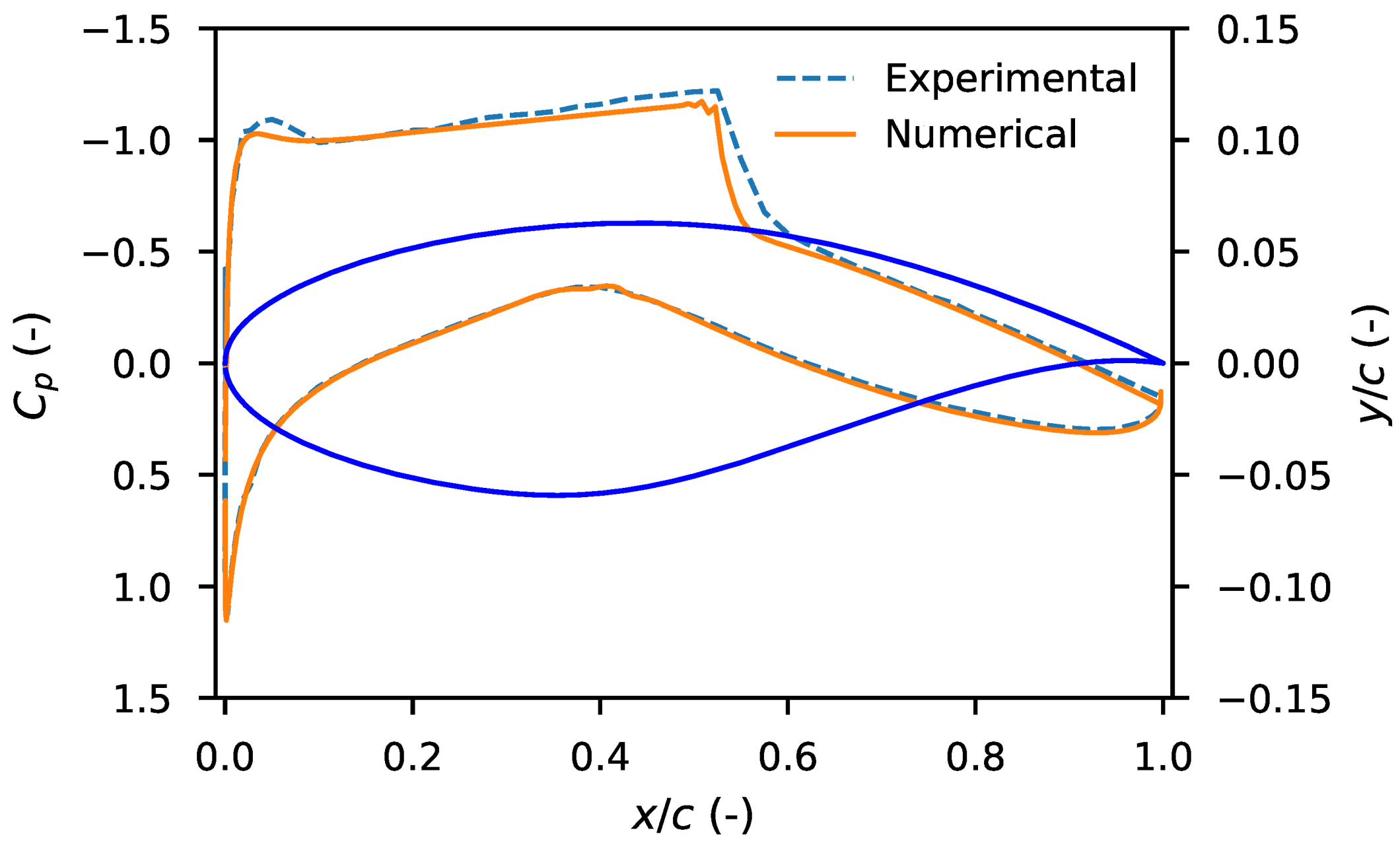
Figure 6.
Comparison of the computational pressure coefficient distribution with the experimental one from [36].
Figure 6.
Comparison of the computational pressure coefficient distribution with the experimental one from [36].

Figure 7.
Control points defined for the FFD method that are used as design variables in the ASO process. The red box marks the hypothetical wing-box which control points remain fixed during the optimization.
Figure 7.
Control points defined for the FFD method that are used as design variables in the ASO process. The red box marks the hypothetical wing-box which control points remain fixed during the optimization.

Figure 8.
Graphical representation of the RAE2822 case of study complemented with the airfoil and wing-box skins.
Figure 8.
Graphical representation of the RAE2822 case of study complemented with the airfoil and wing-box skins.

Figure 9.
Methodology used to apply concentrated loads from discrete pressure values.

Figure 10.
Structural variables’ evolution with the number of nodes.

Figure 11.
Material layout distribution for the general case study, considering 50%, 35%, 25% and 10% mass constraint reduction targets.
Figure 11.
Material layout distribution for the general case study, considering 50%, 35%, 25% and 10% mass constraint reduction targets.

Figure 12.
Pressure coefficient comparison for Case 1.

Figure 13.
Pressure coefficient distribution comparison for case 2.

Figure 14.
von Mises stress distributions (in MPa) for the two case studies and for the original and aerodynamically optimized airfoils.
Figure 14.
von Mises stress distributions (in MPa) for the two case studies and for the original and aerodynamically optimized airfoils.

Figure 15.
Topologically optimized structure for case 1.

Figure 16.
(a) Failure index distribution and (b) von Mises stress distribution for the topologically optimized structure of case 1.
Figure 16.
(a) Failure index distribution and (b) von Mises stress distribution for the topologically optimized structure of case 1.

Figure 17.
Topologically optimized structure for case 2.

Figure 18.
(a) Failure index distribution and (b) von Mises stress distribution for the topologically optimized structure of case 2.
Figure 18.
(a) Failure index distribution and (b) von Mises stress distribution for the topologically optimized structure of case 2.


Table 1.
Mesh convergence study for the CFD simulations.
| Number of Elements (-) | Cl (-) | Cd (Drag Counts) | |
|---|---|---|---|
| Coarse | 43,322 | 0.6737 | 138.8 |
| Medium | 53,492 | 0.7164 | 137.4 |
| Fine | 75,130 | 0.7205 | 130.2 |
| Refined | 85,098 | 0.7215 | 130.5 |
Table 2.
Comparison between the numerical and the experimental results for the RAE2822 airfoil.
| Cl (-) | Cd (Drag Counts) | |
|---|---|---|
| Present Work | 0.7164 | 137.4 |
| Experimental Work [36] | 0.7436 | 127.0 |
Table 3.
Case studies for the RAE2822 airfoil analyzed and optimized in the work.
| Case | Initial (-) | Initial (Drag Counts) |
|---|---|---|
| 1 | 0.7164 | 137.4 |
| 2 | 0.8030 | 183.6 |
Table 4.
Aerodynamic coefficients for the optimized airfoil’s shape.
| Shape | Cl (-) | Cd (Drag Counts) |
|---|---|---|
| Original | 0.7164 | 137.40 |
| Optimized | 0.7164 | 118.23 |
Table 5.
Aerodynamic coefficients for the second case optimized airfoil’s shape.
| Shape | Cl (-) | Cd (Drag Counts) |
|---|---|---|
| Original | 0.803 | 183.62 |
| Optimized | 0.803 | 130.29 |
Table 6.
Structural parameters comparison between the aerodynamically optimized and the original airfoil’s geometries.
Table 6.
Structural parameters comparison between the aerodynamically optimized and the original airfoil’s geometries.
| Case | Geometry | [Pa] | [c] |
|---|---|---|---|
| 1 | Original | ||
| Optimized | |||
| 2 | Original | ||
| Optimized |
Publisher’s Note: MDPI stays neutral with regard to jurisdictional claims in published maps and institutional affiliations. |
© 2021 by the authors. Licensee MDPI, Basel, Switzerland. This article is an open access article distributed under the terms and conditions of the Creative Commons Attribution (CC BY) license (https://creativecommons.org/licenses/by/4.0/).
Share and Cite
MDPI and ACS Style
Gibert Martínez, I.; Afonso, F.; Rodrigues, S.; Lau, F. A Sequential Approach for Aerodynamic Shape Optimization with Topology Optimization of Airfoils. Math. Comput. Appl. 2021, 26, 34. https://doi.org/10.3390/mca26020034
AMA Style
Gibert Martínez I, Afonso F, Rodrigues S, Lau F. A Sequential Approach for Aerodynamic Shape Optimization with Topology Optimization of Airfoils. Mathematical and Computational Applications. 2021; 26(2):34. https://doi.org/10.3390/mca26020034
Chicago/Turabian StyleGibert Martínez, Isaac, Frederico Afonso, Simão Rodrigues, and Fernando Lau. 2021. "A Sequential Approach for Aerodynamic Shape Optimization with Topology Optimization of Airfoils" Mathematical and Computational Applications 26, no. 2: 34. https://doi.org/10.3390/mca26020034