New Stable, Explicit, Shifted-Hopscotch Algorithms for the Heat Equation


1
Institute of Physics and Electrical Engineering, University of Miskolc, 3515 Miskolc, Hungary
2
Department of Mechanical Engineering, University of Technology, 19006 Baghdad, Iraq
*
Author to whom correspondence should be addressed.
Math. Comput. Appl. 2021, 26(3), 61; https://doi.org/10.3390/mca26030061
Submission received: 28 July 2021
/
Revised: 20 August 2021
/
Accepted: 24 August 2021
/
Published: 26 August 2021
Abstract
:Our goal was to find more effective numerical algorithms to solve the heat or diffusion equation. We created new five-stage algorithms by shifting the time of the odd cells in the well-known odd-even hopscotch algorithm by a half time step and applied different formulas in different stages. First, we tested 105 = 100,000 different algorithm combinations in case of small systems with random parameters, and then examined the competitiveness of the best algorithms by testing them in case of large systems against popular solvers. These tests helped us find the top five combinations, and showed that these new methods are, indeed, effective since quite accurate and reliable results were obtained in a very short time. After this, we verified these five methods by reproducing a recently found non-conventional analytical solution of the heat equation, then we demonstrated that the methods worked for nonlinear problems by solving Fisher’s equation. We analytically proved that the methods had second-order accuracy, and also showed that one of the five methods was positivity preserving and the others also had good stability properties.
1. Introduction
Heat and mass transport has a central importance in many scientific and engineering applications. One of the most fundamental ways for these phenomena is the diffusion of heat or particles, described, in the simplest case, by the following linear parabolic partial differential equation (PDE), the so-called heat or diffusion equation. If the medium in which the diffusion takes place is not homogeneous, one can use a more general form.
where, in case of diffusion of particles, denotes the concentration and α is the diffusion coefficient. In the case of conductive heat transfer, u is the temperature and is the thermal diffusivity, while , , and refer to the following nonnegative quantities: heat conductivity, specific heat, and mass density, respectively. These equations and their generalizations, such as the diffusion-convection-reaction equation [1], can describe the diffusive transport of particles in very different physical, chemical, and biological systems, such as in semiconductor devices [2] and the human brain [3]. Furthermore, mathematically similar PDEs can be applied to simulate damped material flow through porous media, such as moisture [4], ground water, crude oil, or natural gas in reservoirs below the Earth’s surface [5]. In this work, we examined only one nonlinear reaction-diffusion equation, the so-called Fisher’s equation [6], apart from the original, linear diffusion equation.
The simple diffusion Equation (1) or more sophisticated equations containing a diffusion term have more and more analytical solutions [7,8,9,10,11,12]. Unfortunately, most of these solutions consider the parameters like the diffusion coefficient or the heat conductivity as constants, which do not depend on space, time, or the dependent variable u. There are counter-examples, such as the work of Zoppou and Knight, in which “analytical solutions have been derived for the two- and three-dimensional advection-diffusion equation with a particular form of the spatially variable coefficients” [13]. However, for space-dependent coefficients in general, one needs to use numerical calculations; therefore, finding effective numerical methods are still important. This is especially true in the nontrivial case of systems where the physical properties are extremely different at different points even in the vicinity of each other [5,14] (p. 15). This often implies that the eigenvalues of the problem have a range of several orders of magnitude; therefore, the problem can be severely stiff. When the PDE is spatially discretized, one obtains a system of ordinary differential equations (ODEs). If the number of variables is very large (which is the case almost always in three space dimensions), the numerical solution of these systems still forms a challenge either by explicit or by implicit methods. It is well known that the traditional explicit methods (such as the Runge–Kutta types) are only conditionally stable, and very small (sometimes unacceptably small) time step sizes have to be applied. Implicit methods are typically unconditionally stable (there are exceptions, e.g., the higher order backward difference methods), but a system of algebraic equations must be solved at each time-step. These calculations can be still very time consuming (note that the matrix is generally not tridiagonal) and, therefore, immense efforts have been made to develop several sophisticated tricks and modifications of the implicit methods (see, e.g., [15] and the references therein). Currently, the implicit methods with these extensions are usually proposed to solve these kinds of problems [16,17,18]. The main obstacle to further progress in the feasibility of large-scale simulations is that the parallelization of these implicit methods are nontrivial, albeit, some progress has been achieved [19,20]. However, there is a tendency towards increasing parallelism in high-performance computing [21,22] due to the halt of the formerly rapid increase of the CPU clock frequencies in the last decades.
Keeping in mind these facts, we are working on the development of novel, easily parallelizable, explicit, and unconditionally stable methods. One of the most important example of these is the two-stage odd-even hopscotch (OEH) algorithm, which was introduced by Gordon [23], then reformulated and analyzed by Gourlay [24,25,26] (see also [27]). This method has been modified to increase its reliability and accuracy, but, as far as we know, always in the direction of a larger extent of implicitness. More concretely, a hierarchy of algorithms was constructed, from the fully explicit OEH through the line hopscotch to the alternating direction implicit (ADI) hopscotch, with increasing accuracy at the expense of programming and running time [25]. These methods were soon applied for the calculation of the heat flow in a thermal print head by Morris and Nicoll. They found that, in case of isotropic media, the OEH method is indeed faster than its more implicit versions with the same accuracy, but in anisotropic cases, the OEH and the line hopscotch give very inaccurate results and the ADI hopscotch is necessary to give a meaningful solution [28]. Later, the OEH method was applied to many problems, e.g., the incompressible Navier–Stokes Equations [29], the Frank–Kamenetskii [30] and the Gray–Scott reaction-diffusion equations [31], and even to the nonlinear Dirac equation [32]. Goede and Boonkkamp applied a vectorized implementation of the OEH scheme to the two-dimensional system of Burgers’ equations and found that the vectorization seriously increased the speed and the obtained solver was very powerful [33]. Recently, Maritim et al. constructed hybrid algorithms containing the hopscotch, the Crank–Nicolson, the Du Fort Frankel, etc. schemes for the two-dimensional system of Burgers’ equations, and concluded that their implicit algorithms are stable and accurate [34,35]. Surprisingly, all modifications of the OEH algorithm increased the level of implicitness and we found no traces of trying to construct similar schemes while keeping the fully explicit property. In our previous paper series [36,37,38], we constructed three new hopscotch combinations by choosing other formulas instead of the original explicit and implicit Euler schemes. The tests showed [36] that, for stiff systems, the original OEH method can produce a so huge inaccuracy for large time step sizes that the relative errors can reach 104, which, in fact, can be more dangerous than instability if not noticed by an inexperienced user. We found that two of the three new combinations behaved much better. In this paper, we extended our research by modifying the underlying space and time structure as well.
The organization of the paper is as follows. In Section 2 we review the OEH structure very briefly and introduce the new algorithms, first for the simplest, one dimensional, equidistant mesh, then, for a general, arbitrary mesh as well. In Section 3, first, we report very concisely the results of the numerical tests for the first assessment of the 105 methods. Then, in Section 3.3 and Section 3.4, we present two numerical experiments in two space-dimensional stiff systems consisting of a large number of cells. Based on the results, we selected the top five combinations with the most valuable properties. In Section 3.5 we verify these five methods by comparing the numerical results produced by them to analytical solutions of the heat equation in one space dimension. The behavior of the algorithms is examined in the case of Fisher’s equation in Section 3.6. Finally, we analyze the convergence and stability properties of these methods. Section 4 will be about the conclusions and our future research goals.
2. The New Methods
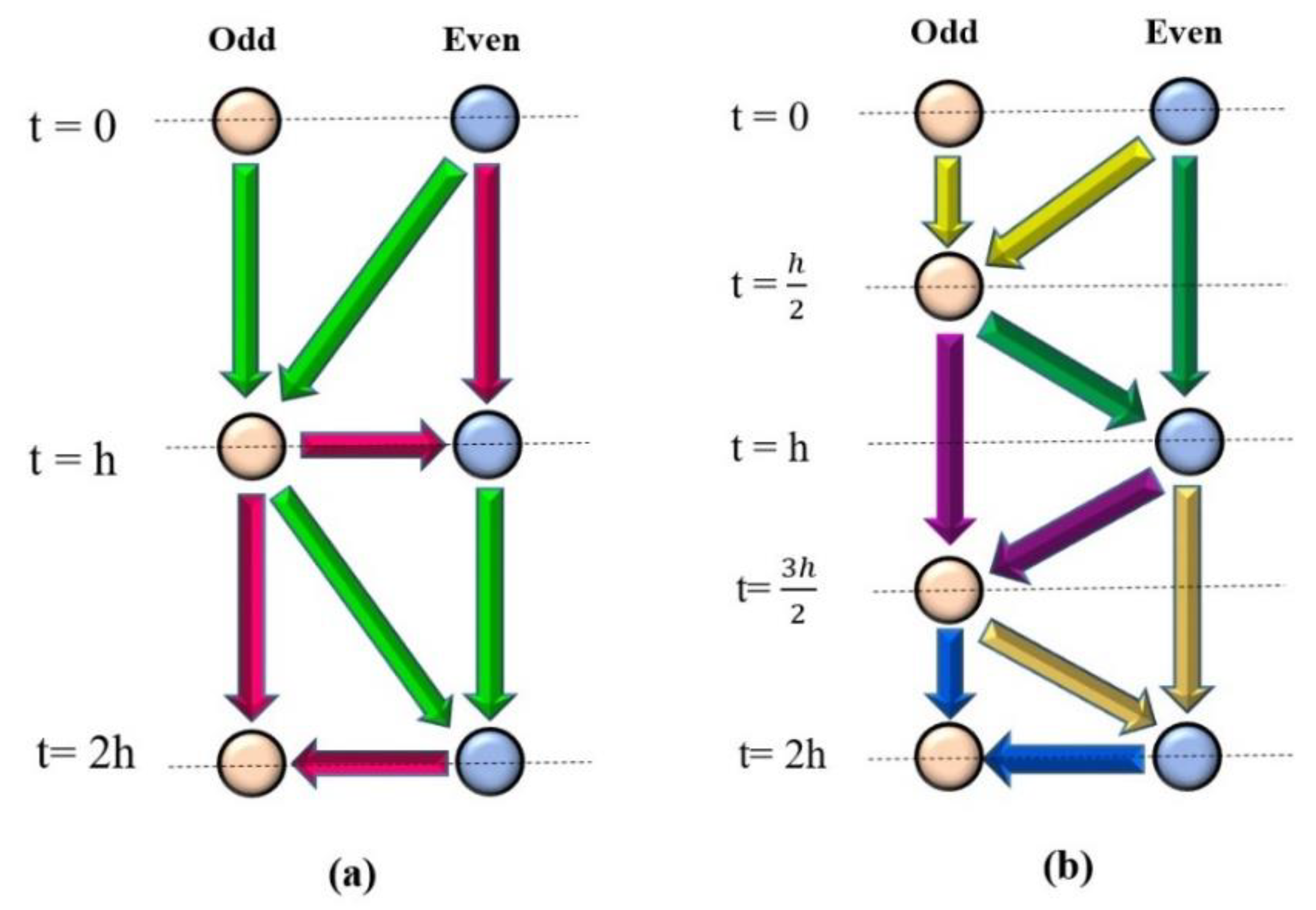
First, we recall the original OEH method for the simple one dimensional equation form of Equation (1). The space and the time variable is discretized by setting nodes according to the most standard rules: , . To introduce the OEH algorithm, we defined a so-called bipartite grid, in which the set of nodes is divided into two similar subsets A and B (with odd and even space index) such that all nearest neighbors of nodes in subset A belong to subset B and vice versa, like on a checkerboard. This space structure is in an intimate connection with the time discretization in the following way. At the first stage of the first time step, the new values of u were calculated only at the points of A, using the latest available values of the neighbors, i.e., the values at the beginning of the time step (see green arrows in Figure 1a). At the second stage, the remaining node values, which belong to subset B, were calculated, using again the latest values at subset A, which were now valid at the end of the time step and already calculated at stage one (red arrows). At the next time step, the roles of subsets A and B were interchanged, etc., as one can see in Figure 1a.
The original OEH method applied the well-known explicit Euler formula at the first stage and the implicit Euler formula at the second stage. However, when the second stage calculations began, the new values of the neighbors and were known, which made the implicit formula effectively explicit. We note, again, that earlier we created new OEH methods by applying different formulas instead of the abovementioned. Now, we modified not only the formulas, but the underlying space and time structure as well, as follows.
The calculation started with taking a half-sized time step for the odd nodes (subset A) using the already calculated values. Then, a full time step was made for the even nodes (subset B), then for the odd cells and the even nodes again. Finally, a half-size time step closed the calculation of the values, as one can see in Figure 1b. In each stage, we used the latest available u values of the neighbors, which meant that the constructed methods were fully explicit and the previous values did not need to be stored at all. Thus, we had a structure consisting of five stages, which corresponded to five partial time steps, which altogether spanned two time steps for odd and even cells, too.
By applying the well-known central difference formula
to Equation (1) in one dimension, a system of ordinary differential equations (ODEs) were obtained for nodes :
The form of this equation for the first and last node depended on the concrete boundary conditions, which will be discussed later. We defined a matrix M with the following elements:
which is tridiagonal in the currently discussed one-dimensional case. Now, equation-system Equation (3) can be written into a condensed matrix-form:
We recall that the following general time discretization
leads to the so-called theta method:
where is the usual mesh ratio and . For one obtains the implicit Euler, the Crank–Nicolson, and the explicit Euler (or, more concretely, the forward-time central-space, FTCS) schemes, respectively [39]. If , the theta method is implicit. Now, in our shifted-hopscotch scheme, the neighbors were always taken into account at the same, latest time level. Thus, we inserted into Equation (6) instead of and , where at the first, middle, and last stages, respectively (see the colored rows in Figure 1b as well). Now, instead of Equation (6) we can write
i.e., our final formula reads as follows:
In the case of , this formula gives back the UPFD method [40,41] with m = n, which takes the form for a half and a full time step, respectively:
The other formula we used was the constant neighbor (CNe) method, which was introduced in our papers [42,43] and now briefly restated here. The starting point is Equation (3), where an approximation is made: When the new value of a variable was calculated, we neglected the fact that the neighbors and were also changing during the time step. It means that the values of uj were considered as constants (that is why we call it constant-neighbor method), so a set of uncoupled ODEs remained:
where the unknowns ui are still functions of the (continuous) time, and a quantity is introduced to collect information about the neighbors of cell i:
These quantities were considered as constant during one time step, but must be recalculated after each time step. The CNe method takes the analytical solution of these simple Equation (10) at the end of the time step or stage to obtain the new values of the u variable:
At the one-dimensional case, this can be written as follows:
At this point, we extended the used methods to general cases where, as happens frequently in real-life problems, the quantities α, k, c, and ρ, describing material properties, are not constants but functions of the space (and time) variables. The interested reader can find more details about this treatment for the case of petroleum reservoirs in Chapter 5 of the book [44]. Let us start with a one-dimensional, still equidistant grid to solve Equation (2). We again discretized the second-order space derivatives by the central difference formula, but now k is a function of x and cannot be simply merged with c and ρ. Thus, we have
Now, we change from node to cell variables, and , , and will be the (average) temperature, specific heat, and density of cell i, respectively, while will be the heat conductivity between cell i and its (right) neighbor. The previous formula will have the form
We go on with a still one-dimensional, but non-equidistant, grid with non-uniform cross section. Let us denote by and the length and the (average) cross section of the cell. One can write the distance between the cell-center of the cell and its arbitrary neighbor j as , and let us approximate the area of the interface between the two neighboring cells as . Using these we can write, more generally than above, that
Now, the volume and the heat capacity of the cell is , and , respectively, while the inverse thermal resistance between these cells can be approximated as . It is obvious that this quantity is zero between non-neighboring cells. Using these new quantities, we obtain the expression for the time derivative of each cell-variable:
which can be easily generalized further to the case with arbitrary number of neighbors:
Let us introduce the characteristic time or time constant τi of cell i as follows:
Here, mii is a diagonal element of the matrix M if we write Equation (13) into the same matrix form as in Equation (5). To restate the used formulas for the general case Equation (13), we introduce the following notations
Now, the general form of Equation (7) is
thus, the generalized theta method for integer time steps reads as follows:
Similarly, the generalized CNe formula is
and, of course, for halved time steps, ri and Ai must be divided by 2.
For the sake of brevity, we will use a compact notation of the individual combinations, where five data are given in a bracket and the numbers are the values of the parameter θ, while the letter ‘C’ is for the CNe constant-neighbor method. For example, (¼, ½, C, ½, ¾) means the following five-stage algorithm will be selected into the top five algorithm in Section 3.3 and named as S2.
Example 1.
Algorithm S2(¼, ½, C, ½, ¾), general from.
Stage 1. Take a half time step with the Equation (16) formula with θ = ¼ for odd cells:
Stage 2. Take a full time step with the Equation (16) formula with θ = ½ for even cells:
Stage 3. Take a full time step with the Equation (17) formula for odd cells:
Stage 4. The same as Stage 2.
Stage 1. Take a half time step with the Equation (16) formula with θ = ¾ for odd cells:
All other combinations can be constructed in this manner straightforwardly.
3. Results
3.1. General Definitions and Circumstances
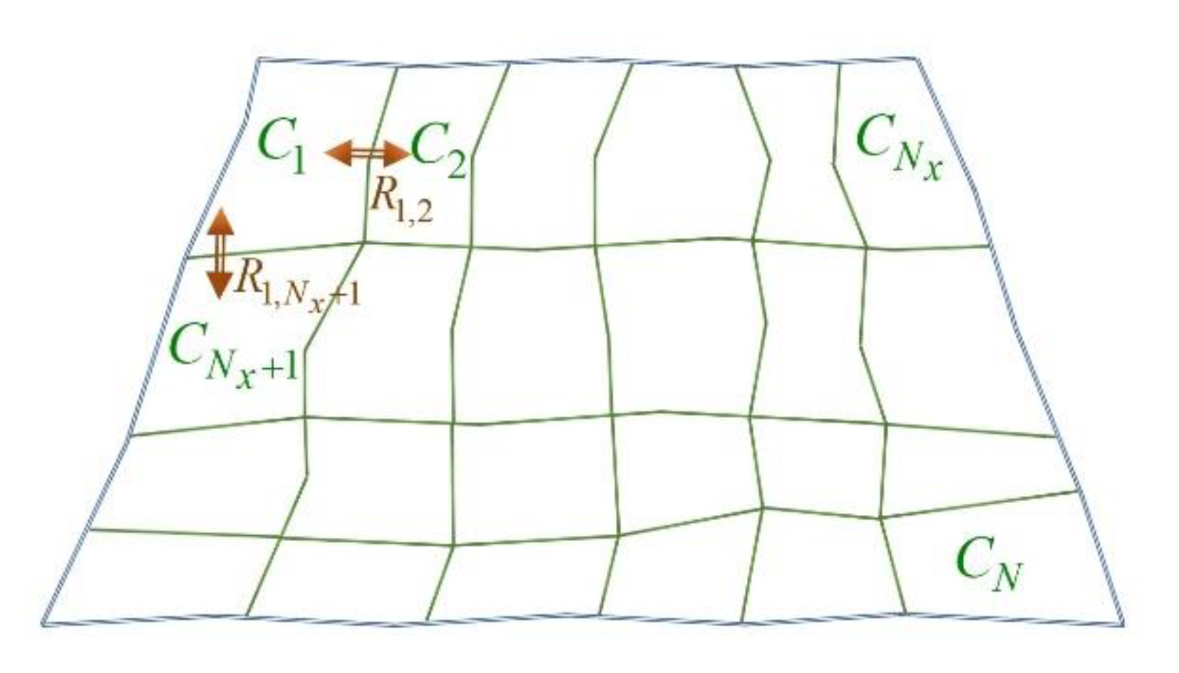
If not stated otherwise, we examined 2-dimensional, rectangle-structured lattices with cells, similar to what can be seen in Figure 2. We solved Equation (13) subjected to randomly generated initial conditions , where rand is a (pseudo)random number with a uniform distribution in the interval (0, 1), generated by the MATLAB for each cell. We also generated different random values for the heat capacities and for the thermal resistances, but with a log-uniform distribution:
where the coefficients in the exponents were concretized later.
We used zero Neumann boundary conditions, i.e., the system was thermally isolated. This was implemented naturally at the level of Equation (13) since it was enough to omit those terms of the sum, which had infinite resistivity in the denominator due to the isolated border. This implied that the system matrix M had one zero eigenvalue, belonging to the uniform distribution of temperatures, and all other eigenvalues must be negative. Let us denote by the (nonzero) smallest (largest) absolute value eigenvalues of matrix M. The stiffness ratio of the system was defined as . The maximum possible time step size for the FTCS (explicit Euler) scheme (from the point of view of stability) was exactly calculated as , above which the solutions were expected to blow up. This threshold time step (often called CFL limit) was essentially valid for the second-order explicit Runge–Kutta (RK) methods as well, since, in the case of them, the border of the stability domain in the negative real axis was the same as for the first-order RK method [45]. We used these two numbers to characterize the “difficulty level” of the problem.
We calculated the numerical error by comparing our numerical solutions with the reference solution at final time . In Section 3.5, the reference solution will be an analytical solution; otherwise, it is a very accurate numerical solution, which has been calculated by the ode15s built-in solver of MATLAB with very strict error tolerance. We used the following three types of (global) error. The first one was the maximum of the absolute differences:
The second one was the average absolute error:
The third one gave the error in terms of energy in case of the heat equation. It took into account that an error of the solution in a cell with a large volume or heat capacity had more significance in practice than in a very small cell
It is well known that the true solution always follows the maximum and minimum principles [39] (p. 87). We say a method is positivity preserving if it never violates this principle, i.e., in our case no value of u was outside of the interval. We were interested in how these errors depend on the time step size in different concrete situations. As one can see in Figure 1, there were five time steps (five stages) altogether, instead of four in the shifted hopscotch structure. Therefore, for the sake of honesty, we had to calculate the effective time step size as , and the errors were plotted as a function of this quantity.
We used a desktop computer with an Intel Core i5-9400 as CPU, 16.0 GB RAM, for the simulations with the MATLAB R2020b software, in which there was a built-in tic-toc function to measure the running time.
3.2. Preliminary Tests
We applied the following nine different values for parameter theta: in Equation (16). It means that, together with the CNe formula, we had 10 different formulas and we inserted all of these into the shifted-hopscotch structure in all possible combinations. As there were five stages in the structure, we had 105 = 100,000 different algorithm-combinations. We wrote a code, which systematically constructed and tested all these combinations. After some tests, we chose the few best combinations, and continued the work only with them. For this, we needed an automatic assessment of the performance of the combinations. The difficulty was in the fact that methods that are very inaccurate or even unstable for large time step sizes can be the most accurate for small time step sizes. Therefore, we chose two different final times, , and calculated the solution with a large time step size (typically ), then repeated the calculation for subsequently halved time step sizes R times until h reached a small value (typically around ). We introduced aggregated relative error (ARE) quantities for each type of errors defined above, which were calculated for the error as follows:
which means that was the average of the difference between the error of the original OEH method and the actual shifted combination in terms of orders of magnitude. Then the code calculated the simple average of these errors:
and finally sorted the 100,000 combinations in descending order, according to this quantity. In the obtained list, usually positive ARE values were assigned the first few thousands of combinations, with the largest ones typically around 2, which means that some combinations were roughly two orders of magnitude more accurate than the original OEH method. We performed this procedure in the case of four different small systems with . The parameters of the distribution of the mesh-cells data were chosen to construct test problems with various stiffness ratios and , for example, . We give the best 12 combinations in their short form:
(0, ½, ½, ½, 1), (½, ½, ½, ½, ½), (0, C, ½, C, 1), (0, C, C, C, 1),
(¾, ⅔, ½, ⅓, ¼), (¼, ½, C, ½, ¾), (⅓, ⅔, C, ⅓, ⅔), (C, ½, C, ½, C),
(⅕, ½, ½, ½, ⅘), (¼, ½, ½, ½, ¾), (⅓, ½, ½, ½, ⅔), (0, ½, ½, C, 1).
(¾, ⅔, ½, ⅓, ¼), (¼, ½, C, ½, ¾), (⅓, ⅔, C, ⅓, ⅔), (C, ½, C, ½, C),
(⅕, ½, ½, ½, ⅘), (¼, ½, ½, ½, ¾), (⅓, ½, ½, ½, ⅔), (0, ½, ½, C, 1).
Later, we proved that formulas θ = 1 and CNe preserved positivity of the solution and, therefore, if only these two formulas are used in a combination, the whole algorithm will preserve positivity. Since this property is considered valuable [40,46], we repeated the above experiments for these 25 = 32 combinations (instead of the 100,000 above). We concluded that the (C, C, C, C, C) combination was the most accurate among these; therefore, we further investigate d13 combinations altogether. We emphasize that these are the results of only preliminary (one might say tentative) tests, with the sole purpose of reducing the huge number of combinations into a manageable number, and we have not stated anything exactly until this point.
3.3. Case Study I and Comparison with Other Solvers
We examined a grid similar to the one in Figure 2 with isolated boundary, but the sizes were fixed to and ; thus, the total cell number was 10,000, while the final time was . The exponents introduced above were set to the following values
which means that log-uniformly distributed values between 0.01 and 100 were given to the capacities. The generated system can be characterized by its stiffness ratio and values, which are and , respectively. The performance of new algorithms was compared with all available MATLAB solvers:
- ode15s, a first- to fifth-order (implicit) numerical differentiation formula with variable step and variable order (VSVO), developed for solving stiff problems;
- ode23s, a second-order modified (implicit) Rosenbrock formula;
- ode23t, applies (implicit) trapezoidal rule with using free interpolant;
- ode23tb, combines backward differentiation formula and trapezoidal rule;
- ode45, a fourth/fifth-order explicit Runge–Kutta–Dormand–Prince formula;
- ode23, second/third-order explicit Runge–Kutta–Bogacki–Shampine method;
- ode113, first- to 13th- order VSVO Adams–Bashforth–Moulton numerical solver.
For all used MATLAB solvers, tolerances were changed over many orders of magnitude, from the maximum value to the minimum value . We also used the following methods for comparison purposes. The original UPFD, the CNe method, and the Dufort–Frankel (DF) algorithm
are explicit unconditionally stable schemes. The DF scheme is a two-step method, which is not self-starter; thus, we calculated the first time step by two subsequent UPFD steps with halved time step sizes. Finally, the widely used Crank–Nicolson (CN) is a widely used implicit scheme:
where I is the unit matrix. The A and B matrixes did not depend on time here, so they were calculated only once, before the first time step. This scheme was implemented two different ways: by calculating before the first time step and then each time step was just a simple matrix multiplication , which is denoted by ‘CrN invert’, and by the command, which is denoted by ‘CrN lins’. One will see that this implicit method was still very slow for the actual system size.
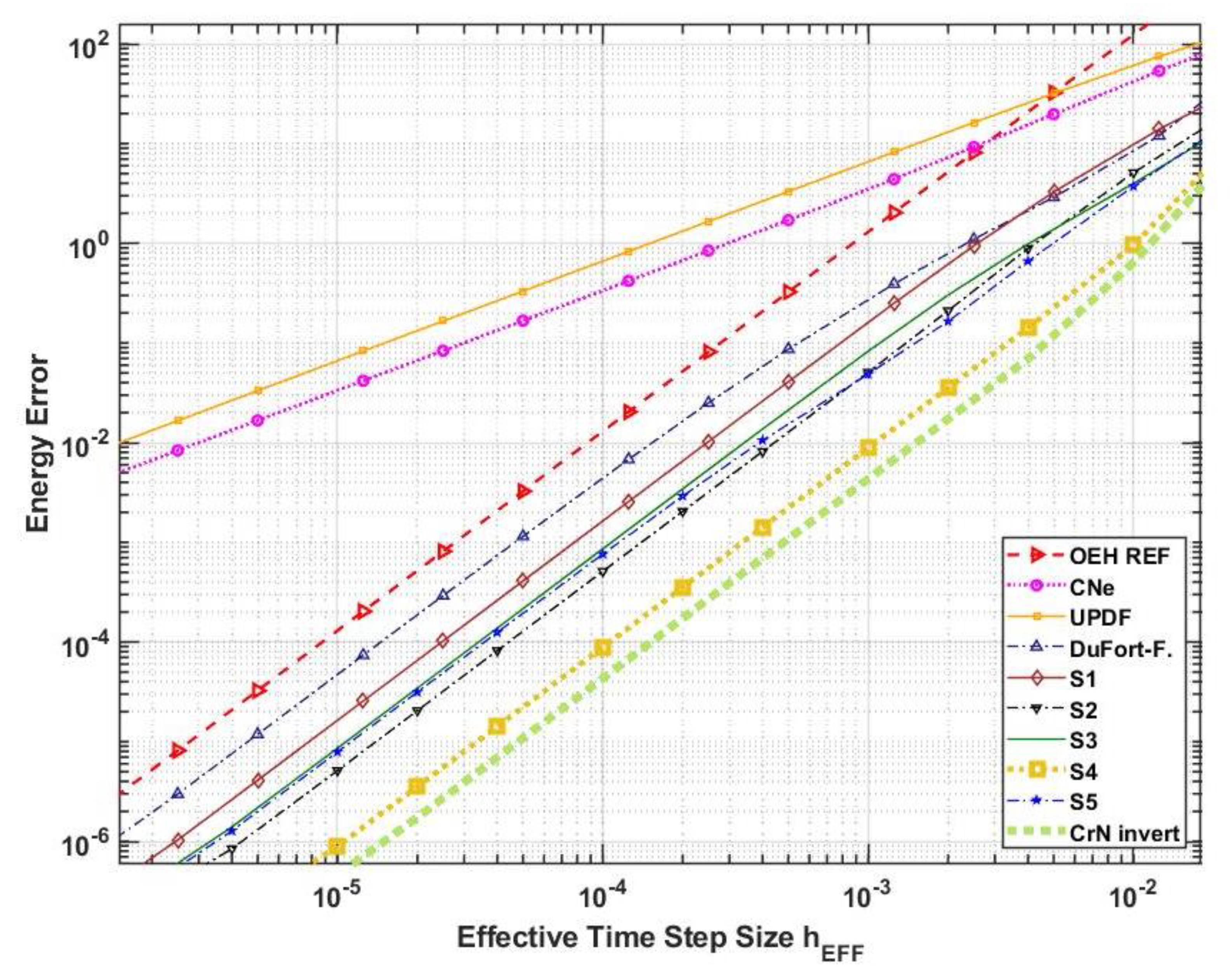
We plotted the , the , and the energy errors as a function of the effective time step size , and, based on this (and on similar data belonging to the more stiff system in the next subsection), we selected the following top five combinations from those listed in Equation (24) and after that:
S1 (C, C, C, C, C),
S2 (¼, ½, C, ½, ¾),
S3 (¼, ½, ½, ½, ¾),
S4 (0, ½, ½, ½, 1),
S5 (0, ½, ½, C, 1)
S2 (¼, ½, C, ½, ¾),
S3 (¼, ½, ½, ½, ¾),
S4 (0, ½, ½, ½, 1),
S5 (0, ½, ½, C, 1)
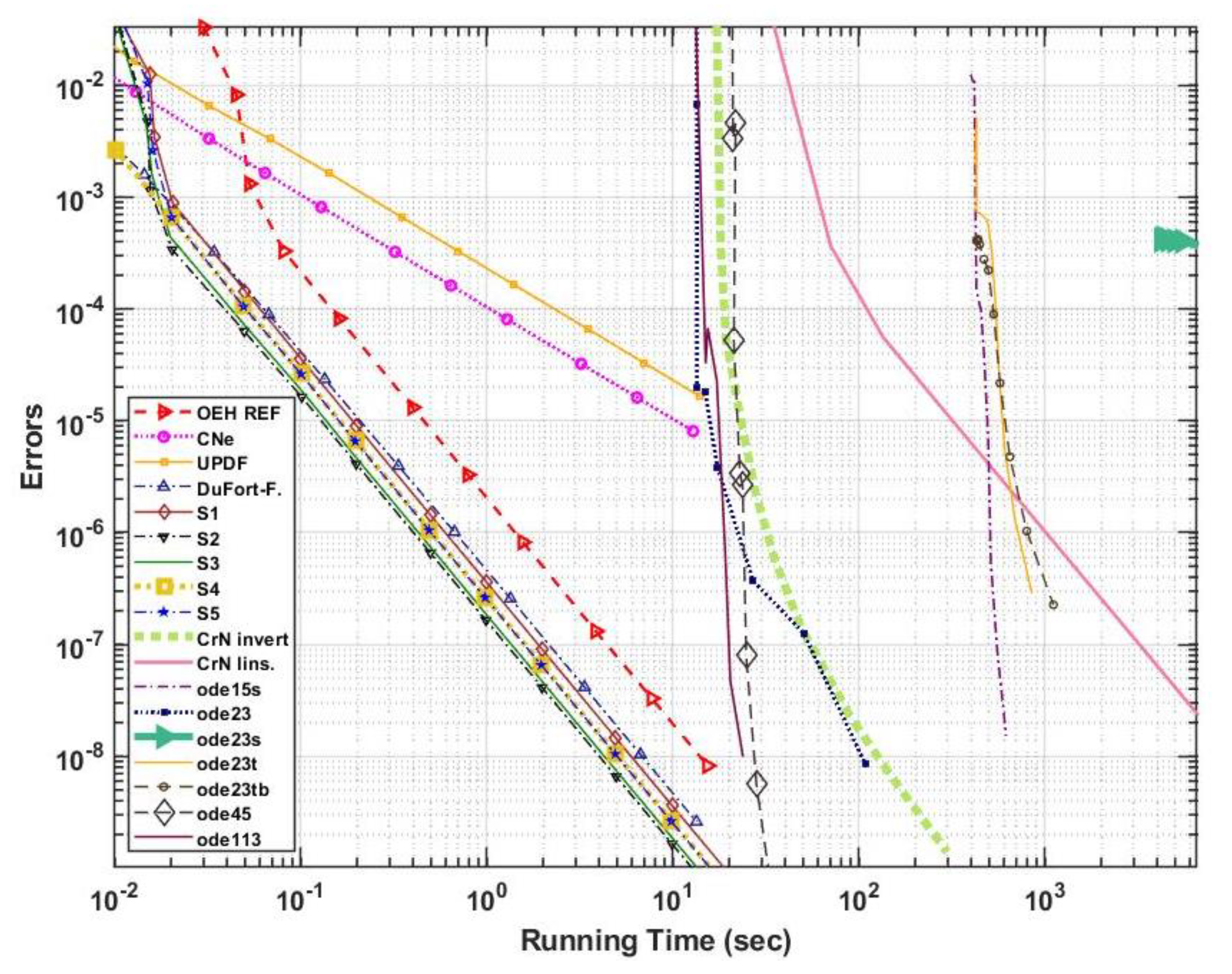
In Figure 3, we present the error functions only for these top five combinations and some other, known methods, while in Figure 4 and Figure 5 one can see the and the energy errors vs. the total running times. Furthermore, Table 1 presents some results that were obtained by our numerical schemes, the two implementations of the Crank–Nicolson method and the “ode” routines of MATLAB.
3.4. Case Study II and Comparison with Other Solvers
We tested our new algorithms and the conventional solvers for a harder problem as well. Thus, new values were set for the α and β exponents:
This means that the width of the distribution of the capacities and thermal resistances were increased. Now, the largest capacity was six orders or magnitude larger than the smallest one. The system acquired some anisotropy as well, since the resistances in the x direction were two orders of magnitude larger than in the z direction, on average, . With this modification we gained a system with a much higher stiffness ratio, , while the maximum allowed time step size for the standard FTCS was . All other parameters and circumstances remained the same as in Section 3.3. In Figure 6 and Figure 7, energy errors and the errors are presented as a function of the time step size and the total running time, respectively, while in Table 2 some results are collected for the same system.
One can see that the implicit MATLAB solvers performed much better than the explicit ones, unlike in the previous case. As all of our cases had considerable stiffness, the implicit Crank–Nicolson method was more accurate than our explicit methods, but the difference was not always large. On the other hand, all implicit methods required much longer time for running than the unconditionally stable explicit algorithms. However, we remind the reader that this system of 10,000 cells was still rather small, and, for a growing number of cells, the implicit methods have an increasing disadvantage. Moreover, the performance of the standard explicit solvers declined with increasing stiffness, so solving very large and stiff systems is a very tough problem. In Figure 7, the otherwise very powerful ode45 solver is represented only by one point (right side of the figure) because, for large tolerances, it diverged, while for low tolerances, the running of the program was stopped by an error message. In fact, we did not test our methods in the case of larger systems (with 20,000 or more cells) because no solvers of MATLAB could produce a reference solution.
3.5. Verification by Comparison to Analytical Results
We considered very recent nontrivial analytical solutions of Equation (1) found by Barna and Mátyás [10] by a similarity transformation technique. Both of them are given, on the whole, a real number line for positive values of t, as follows
and
We reproduced these solutions only in finite space and time intervals and , where . The space interval was discretized by creating nodes as follows: . We prescribed the appropriate Dirichlet boundary conditions at the two ends of the interval:
and
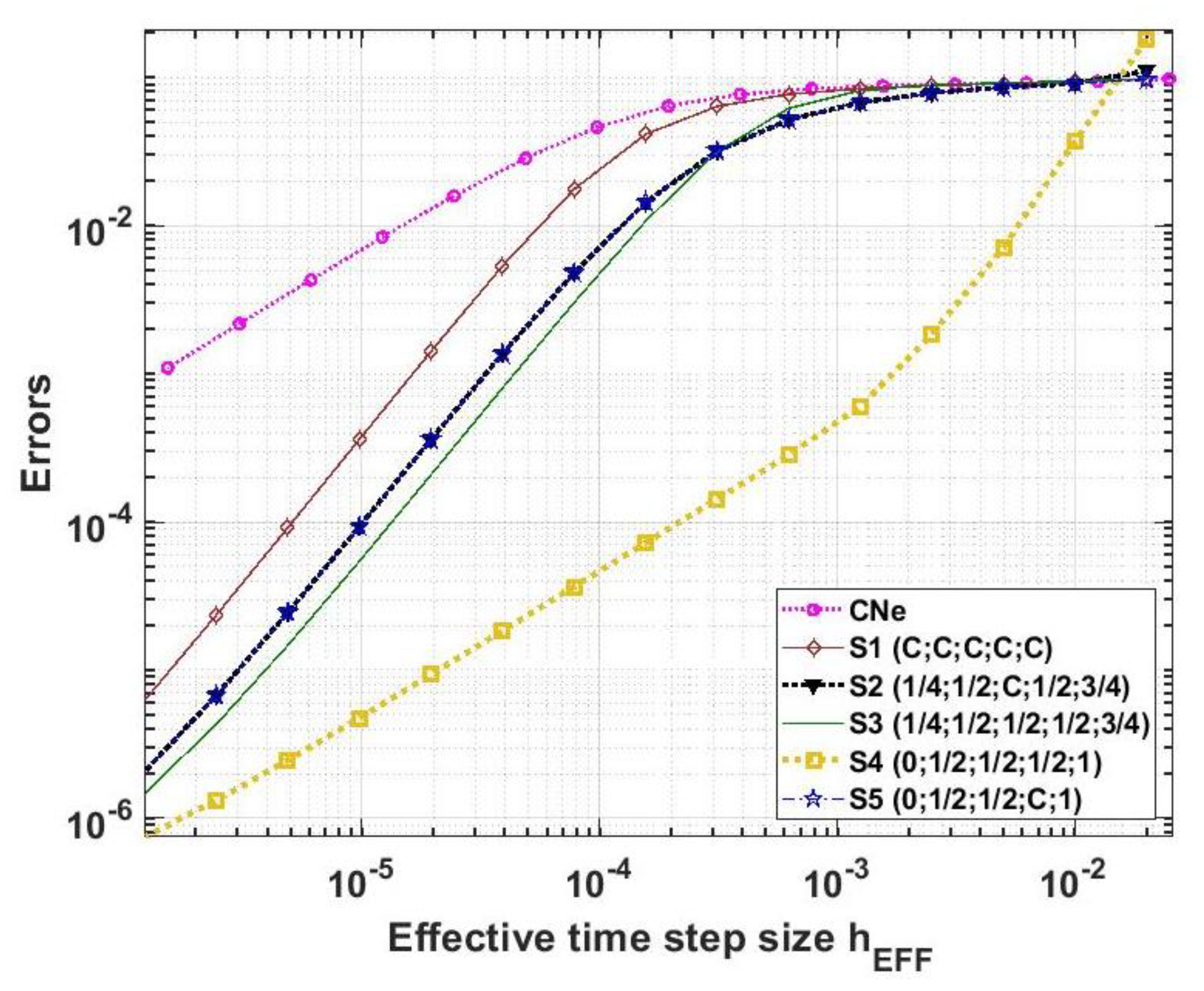
where . We obtained that the new methods were convergent and the order of convergence was 2. In Figure 8, the errors as a function of the effective time step size hEFF are presented for the case of the u2 solution for the top five algorithms and a first-order “reference curve” for the original CNe method. We note that very similar curves were obtained for the u1 solution, as well as for other space and time intervals.
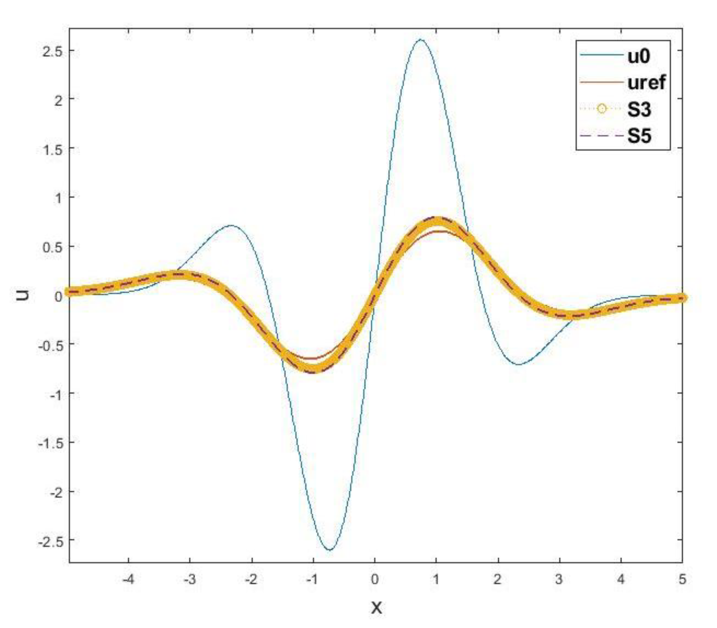
We also present the graphs of the initial function , the analytical solution , and two corresponding numerical solutions for in Figure 9. We emphasize that, at this time step size range, the algorithm S4 was the most accurate, but we did not present its graph, as it would be completely indistinguishable from the exact solution.
3.6. Verification for the Nonlinear Fisher’s Equation
We considered
for α = 1 and solved it, subject to the following initial condition:
The Dirichlet boundary conditions appropriate to the exact solution were prescribed at both ends of the interval:
We reproduced this analytical solution in the case of several values of the parameters , and , but here we present results only for , and . In order to have good stability properties, we took account the effect of the nonlinear term via the following semi-implicit treatment
which can be rearranged into a fully explicit form:
where is the actual value of after performing the previous stage calculations, which deal with the diffusion term. This operation was performed in two extra, separate stages, where a loop was going through all the nodes (both odd and even). The first extra stage was after (the original) Stage 2, while the second was after Stage 4, at the same moments in which the boundary conditions were refreshed.
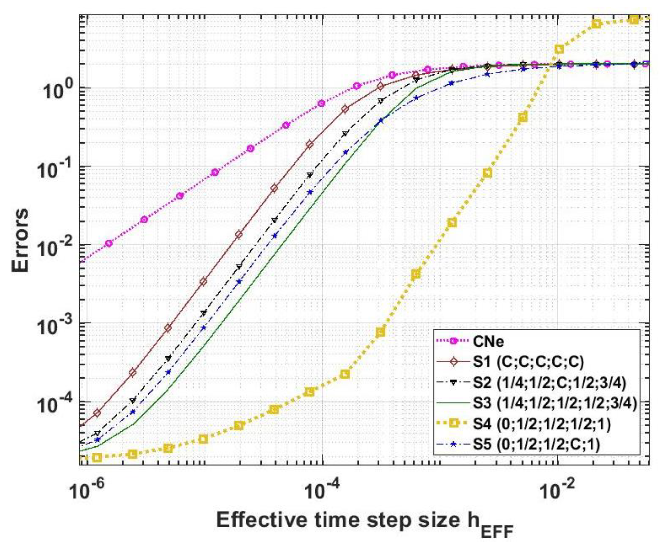
With this procedure we obtained that the new methods behaved very similarly as in the linear case. In Figure 10, the errors as a function of the effective time step size hEFF are presented for the top five algorithms and the original CNe method. We note that very similar curves were obtained for other space and time intervals and values of parameter β.
We emphasize that this subsection is only to demonstrate that these shifted-hopscotch methods can be successfully applied for other, possibly nonlinear, equations as well, and there is some chance that the relative strength of the S1–S5 algorithms is preserved. The systematic investigation of the behavior of the new methods in case of nonlinear equations was out of the scope of this paper and plans to be published in future works.
3.7. Analytical Investigations
We started with the analysis of the convergence properties of the five most advantageous methods in the one-dimensional case for constant values of mesh ratio r: In other words, when the equidistant spatial discretization was fixed.
Theorem 1.
The order of convergence of the S1…S5 shifted hopscotch algorithms is 2 for the Equation (5) system of linear ODEs:
where M is defined in Equation (4) and is an arbitrary vector.
The proof is presented in the Appendix A. Now, we turn our attention to the question of stability. First, we examined the two types of formulas (the UPFD and the CNe), about which we already stated that they are positivity preserving.
Lemma 1.
The newvalues are the convex combinations of the old values in Equations (9), (11) and (17) formulas, as well as in the Equation (16) formula for.
The proofs of these statements are very easy, and they are given in our previous papers (see Theorem 2 in [37] for the UPFD and also Theorem 2 in [43] for the CNe). We also recalled a lemma on the associativity of convex combinations [47] (p. 28).
Lemma 2.
A convex combinationof convex combinations is again a convex combination:
for any .
Corollary 1.
All shifted hopscotch algorithms containing only the CNe and the UPFD formulas mentioned in Lemma 1, the new values are the convex combinations of the old values.
This immediately implies that all algorithms mentioned in Corollary 1, especially S1 (C, C, C, C, C), followed the minimum and maximum principle, and, therefore, preserved positivity, which is a much stronger property than unconditional stability.
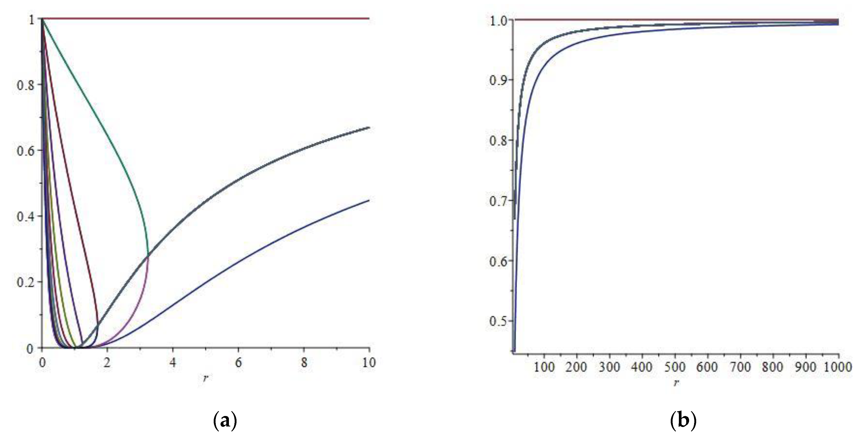
We examined the stability of the S2–S5 algorithms through their eigenvalues. We constructed the five stages of these algorithms in a matrix form. If we denote these matrices by M1,…, M5, respectively, the matrix of a two-step, five-stage algorithm can be written as , and . We calculated and plotted the absolute values of the eigenvalues of this matrix H as a function of the mesh ratio r for several values of N, and found that the largest one was always exactly 1, which implies that no perturbation vector could grow unboundedly. In Figure 11, we present here only the eigenvalue functions of S4 (0, ½, ½, ½, 1), which produced the largest errors for large time step sizes (see, e.g., the top right corner of Figure 8) and, therefore, one might question its stability first. These results verify that the S2…S4 methods were unconditionally stable, even if they could not be considered as exact analytical proofs.
4. Discussion and Summary
In this article, we constructed and tested novel numerical algorithms to solve the non-stationary diffusion (or heat) equation. The new algorithms were fully explicit time-integrators obtained by applying half and full time steps in the odd-even hopscotch structure. All of the algorithms consisted of five stages, but they were one-step methods in the sense that when the new values of the unknown function u were calculated, only the most recently calculated u values were used. Thus, the methods could be implemented such that only one array of storage was required for the u variable, which means that the memory requirement was very low. We applied the conventional theta method with nine different values of and the non-conventional CNe method to construct 105 combinations and chose the top five of them via numerical experiments. We showed concrete results of these five algorithms in the case of two 2-dimensional stiff systems containing 10,000 cells with highly inhomogeneous, randomly generated parameters and discontinuous initial conditions. These experiments suggest that the proposed methods are, indeed, competitive, as they can give fairly accurate results orders of magnitude faster than the well-optimized MATLAB routines or the Crank–Nicolson method, and they are also significantly more accurate for stiff systems than the UPFD, the Dufort–Frankel, or the original odd-even hopscotch method. We think that, if high accuracy is required, the S4 (0, ½, ½, ½, 1) combination can be proposed; however, when preserving positivity is crucial, the S1 (C, C, C, C, C) algorithm should be used.
We verified these new algorithms by reproducing a recently found nontrivial analytical solution of the heat equation, and then also showed that the nonlinear Fisher’s equation can be solved by them. We proved analytically that the new methods are second order for fixed spatial discretization. It must be noted that the original explicit Euler, UPFD, and CNe formulas are only first order and the shifted-hopscotch structure made their combinations second order. On the other hand, the original theta method for (which is the trapezoidal rule) is second order, but it is either an implicit method (the CN scheme) or, if made explicit by a predictor step, it requires an extra (predictor) stage and, at the same time, becomes only conditionally stable. At the end of the paper, we conveyed evidence about the good stability properties of the new methods.
In our next papers we would like to extend our investigations in order to find even more effective algorithms and perform more comprehensive tests to clarify which are the best under specific circumstances. Then, we also plan to apply the methods for more complicated, mostly nonlinear equations, as well as in case of real-life engineering problems such as heat transfer by conduction and radiation in buildings or machine tools. We already started the application of the methods to equations where additional terms are present besides the diffusion term, such as the advection-diffusion and the Kardar–Parisi–Zhang equations, but these investigations are still at an embryonic stage. In principle, the shifted hopscotch structure and the concrete proposed methods can be adapted to hyperbolic equations like the Euler equations as well, but we have doubts about their stability properties under those circumstances.
Author Contributions
Conceptualization, E.K. and H.K.; methodology, E.K. and M.S.; software, Á.N. and I.O.; validation, E.K., H.K. and I.O.; formal analysis, M.S.; investigation, Á.N., I.O. and H.K.; resources, E.K.; data curation, Á.N.; writing—original draft preparation, E.K. and M.S.; writing—review and editing, E.K. and Á.N.; visualization, Á.N. and I.O.; supervision, E.K.; project administration, E.K. and Á.N. All authors have read and agreed to the published version of the manuscript.
Funding
This research received no external funding.
Data Availability Statement
Data are available at the following link: http://dx.doi.org/10.17632/sdxrxf68jg.1#folder-649cdd07-097d-43de-b61b-87a74f9b2eec (accessed on 24 August 2021).
Conflicts of Interest
The authors declare no conflict of interest.
Appendix A
Proof of Theorem 1.
First, we give the general form of the new vector elements expressed by the old elements for odd and even cells far from the boundaries for the top 5 algorithms.
S1 (C, C, C, C, C), i is odd:
S1 (C, C, C, C, C), i is even:
S2 (¼, ½, C, ½, ¾), i is odd:
S2 (¼, ½, C, ½, ¾), i is even:
S3 (¼, ½, ½, ½, ¾), i is odd:
S3 (¼, ½, ½, ½, ¾), i is even:
S4 (0, ½, ½, ½, 1), i is odd:
S4 (0, ½, ½, ½, 1), i is even:
S5 (0, ½, ½, C, 1), i is odd:
S5 (0, ½, ½, C, 1), i is even:
We have to show that the zeroth-, first-, and second-order local errors are zero, i.e., the numerical solution is identical to the exact solution of the PDE initial value problem Equation (A1) up to second order. We will use the usual series expansion up to second order
The exact solution at the end of a doubled time step is the following:
After some simple algebraic calculations, we obtain:
Now we calculate the coefficients of Equation (A1) up to the second order:
Substituting these terms into Equation (A1) we obtain
It can be immediately seen that this expression is identical to the analytical solution Equation (A12) up to second order. Equation (A2) can be handled similarly to obtain the same expression as in Equation (A12) or (A14), which proves the theorem for the S1 algorithm. For the S2…S5 methods we use the power series expansion , so we have
etc. These expressions can be substituted back to Equations (A3) and (A4) to obtain Equation (A14) again. In the same manner, we proved the second-order property of algorithms S3…S5, which is not detailed here, being even more trivial than the case of S1 and S2. □
References
- Zhong, J.; Zeng, C.; Yuan, Y.; Zhang, Y.; Zhang, Y. Numerical solution of the unsteady diffusion-convection-reaction equation based on improved spectral Galerkin method. AIP Adv. 2018, 8, 045314. [Google Scholar] [CrossRef]
- Blaj, G.; Kenney, C.J.; Segal, J.; Haller, G. Analytical Solutions of Transient Drift-Diffusion in P–N Junction Pixel Sensors. arXiv 2017, arXiv:1706.01429. [Google Scholar]
- Le Bihan, D. Diffusion MRI: What water tells us about the brain. EMBO Mol. Med. 2014, 6, 569–573. [Google Scholar] [CrossRef] [PubMed]
- Gasparin, S.; Berger, J.; Dutykh, D.; Mendes, N. Stable explicit schemes for simulation of nonlinear moisture transfer in porous materials. J. Build. Perform. Simul. 2018, 11, 129–144. [Google Scholar] [CrossRef] [Green Version]
- Zimmerman, R.W. The Imperial College Lectures in Petroleum Engineering; World Scientific Publishing: Singapore; London, UK, 2018; ISBN 9781786345004. [Google Scholar]
- Fisher, R.A. The Wave of Advance of Advantageous Genes. Ann. Eugen. 1937, 7, 355–369. [Google Scholar] [CrossRef] [Green Version]
- Mojtabi, A.; Deville, M.O. One-dimensional linear advection-diffusion equation: Analytical and finite element solutions. Comput. Fluids 2015, 107, 189–195. [Google Scholar] [CrossRef] [Green Version]
- Barna, I.F.; Bognár, G.; Guedda, M.; Mátyás, L.; Hriczó, K. Analytic self-similar solutions of the Kardar–Parisi–Zhang interface growing equation with various noise terms. Math. Model. Anal. 2020, 25, 241–256. [Google Scholar] [CrossRef]
- Barna, I.F.; Kersner, R. Heat conduction: A telegraph-type model with self-similar behavior of solutions. J. Phys. A Math. Theor. 2010, 43, 375210. [Google Scholar] [CrossRef]
- Mátyás, L.; Barna, I.F. General self-similar solutions of diffusion equation and related constructions. arXiv 2021, arXiv:2104.09128. [Google Scholar]
- Bastani, M.; Salkuyeh, D.K. A highly accurate method to solve Fisher’s equation. Pramana J. Phys. 2012, 78, 335–346. [Google Scholar] [CrossRef]
- Agbavon, K.M.; Appadu, A.R.; Khumalo, M. On the numerical solution of Fisher’s equation with coefficient of diffusion term much smaller than coefficient of reaction term. Adv. Differ. Eq. 2019, 146. [Google Scholar] [CrossRef]
- Zoppou, C.; Knight, J.H. Analytical solution of a spatially variable coefficient advection-diffusion equation in up to three dimensions. Appl. Math. Model. 1999, 23, 667–685. [Google Scholar] [CrossRef]
- Lienhard, J.H., IV; Lienhard, J.H., V. A Heat Transfer Textbook, 4th ed.; Phlogiston Press: Cambridge, MA, USA, 2017; ISBN 9780971383524. [Google Scholar]
- Cusini, M. Dynamic Multilevel Methods for Simulation of Multiphase Flow in Heterogeneous Porous Media; Delft University of Technology: Delft, The Netherlands, 2019. [Google Scholar]
- Appau, P.O.; Dankwa, O.K.; Brantson, E.T. A comparative study between finite difference explicit and implicit method for predicting pressure distribution in a petroleum reservoir. Int. J. Eng. Sci. Technol. 2019, 11, 23–40. [Google Scholar] [CrossRef] [Green Version]
- Moncorgé, A.; Tchelepi, H.A.; Jenny, P. Modified sequential fully implicit scheme for compositional flow simulation. J. Comput. Phys. 2017, 337, 98–115. [Google Scholar] [CrossRef]
- Chou, C.S.; Zhang, Y.T.; Zhao, R.; Nie, Q. Numerical methods for stiff reaction-diffusion systems. Discret. Contin. Dyn. Syst. Ser. B 2007, 7, 515–525. [Google Scholar] [CrossRef]
- Gumel, A.B.; Ang, W.T.; Twizell, E.H. Efficient parallel algorithm for the two-dimensional diffusion equation subject to specification of mass. Int. J. Comput. Math. 1997, 64, 153–163. [Google Scholar] [CrossRef]
- Xue, G.; Feng, H. A new parallel algorithm for solving parabolic equations. Adv. Differ. Eq. 2018, 2018, 1–6. [Google Scholar] [CrossRef] [Green Version]
- Gagliardi, F.; Moreto, M.; Olivieri, M.; Valero, M. The international race towards Exascale in Europe. CCF Trans. High Perform. Comput. 2019, 3–13. [Google Scholar] [CrossRef] [Green Version]
- Reguly, I.Z.; Mudalige, G.R. Productivity, performance, and portability for computational fluid dynamics applications. Comput. Fluids 2020, 199, 104425. [Google Scholar] [CrossRef]
- Gordon, P. Nonsymmetric Difference Equations. J. Soc. Ind. Appl. Math. 1965, 13, 667–673. [Google Scholar] [CrossRef]
- Gourlay, A.R. Hopscotch: A Fast Second-order Partial Differential Equation Solver. IMA J. Appl. Math. 1970, 6, 375–390. [Google Scholar] [CrossRef]
- Gourlay, A.R.; McGuire, G.R. General Hopscotch Algorithm for the Numerical Solution of Partial Differential Equations. IMA J. Appl. Math. 1971, 7, 216–227. [Google Scholar] [CrossRef]
- Gourlay, A.R. Some recent methods for the numerical solution of time-dependent partial differential equations. Proc. R. Soc. Lond. A Math. Phys. Sci. 1971, 323, 219–235. [Google Scholar] [CrossRef]
- Hundsdorfer, W.H.; Verwer, J.G. Numerical Solution of Time-Dependent Advection-Diffusion-Reaction Equations; Springer: Berlin, Germany, 2003. [Google Scholar]
- Morris, J.L.; Nicoll, I.F. Hopscotch methods for an anisotropic thermal print head problem. J. Comput. Phys. 1973, 13, 316–337. [Google Scholar] [CrossRef]
- ten Thije Boonkkamp, J.H.M. The Odd-Even Hopscotch Pressure Correction Scheme for the Incompressible Navier–Stokes Equations. SIAM J. Sci. Stat. Comput. 1988, 9, 252–270. [Google Scholar] [CrossRef]
- Harley, C. Hopscotch method: The numerical solution of the Frank–Kamenetskii partial differential equation. Appl. Math. Comput. 2010, 217, 4065–4075. [Google Scholar] [CrossRef]
- Al-Bayati, A.; Manaa, S.; Al-Rozbayani, A. Comparison of Finite Difference Solution Methods for Reaction Diffusion System in Two Dimensions. AL-Rafidain J. Comput. Sci. Math. 2011, 8, 21–36. [Google Scholar] [CrossRef] [Green Version]
- Xu, J.; Shao, S.; Tang, H. Numerical methods for nonlinear Dirac equation. J. Comput. Phys. 2013, 245, 131–149. [Google Scholar] [CrossRef] [Green Version]
- de Goede, E.D.; ten Thije Boonkkamp, J.H.M. Vectorization of the Odd–Even Hopscotch Scheme and the Alternating Direction Implicit Scheme for the Two-Dimensional Burgers Equations. SIAM J. Sci. Stat. Comput. 1990, 11, 354–367. [Google Scholar] [CrossRef]
- Maritim, S.; Rotich, J.K.; Bitok, J.K. Hybrid hopscotch Crank–Nicholson-Du Fort and Frankel (HP-CN-DF) method for solving two dimensional system of Burgers’ equation. Appl. Math. Sci. 2018, 12, 935–949. [Google Scholar] [CrossRef]
- Maritim, S.; Rotich, J.K. Hybrid Hopscotch Method for Solving Two Dimensional System of Burgers’ Equation. Int. J. Sci. Res. 2018, 8, 492–497. [Google Scholar]
- Saleh, M.; Nagy, Á.; Kovács, E. Construction and investigation of new numerical algorithms for the heat equation: Part 1. Multidiszcip. Tudományok 2020, 10, 323–338. [Google Scholar] [CrossRef]
- Saleh, M.; Nagy, Á.; Kovács, E. Construction and investigation of new numerical algorithms for the heat equation: Part 2. Multidiszcip. Tudományok 2020, 10, 339–348. [Google Scholar] [CrossRef]
- Saleh, M.; Nagy, Á.; Kovács, E. Construction and investigation of new numerical algorithms for the heat equation: Part 3. Multidiszcip. Tudományok 2020, 10, 349–360. [Google Scholar] [CrossRef]
- Holmes, M.H. Introduction to Numerical Methods in Differential Equations; Springer: New York, NY, USA, 2007. [Google Scholar]
- Chen-Charpentier, B.M.; Kojouharov, H.V. An unconditionally positivity preserving scheme for advection-diffusion reaction equations. Math. Comput. Model. 2013, 57, 2177–2185. [Google Scholar] [CrossRef]
- Appadu, A.R. Performance of UPFD scheme under some different regimes of advection, diffusion and reaction. Int. J. Numer. Methods Heat Fluid Flow 2017, 27, 1412–1429. [Google Scholar] [CrossRef] [Green Version]
- Kovács, E. New Stable, Explicit, First Order Method to Solve the Heat Conduction Equation. J. Comput. Appl. Mech. 2020, 15, 3–13. [Google Scholar] [CrossRef]
- Kovács, E. A class of new stable, explicit methods to solve the non-stationary heat equation. Numer. Methods Partial Differ. Eq. 2020, 37, 2469–2489. [Google Scholar] [CrossRef]
- Munka, M.; Pápay, J. 4D Numerical Modeling of Petroleum Reservoir Recovery; Akadémiai Kiadó: Budapest, Hungary, 2001; ISBN 963-05-7843-3. [Google Scholar]
- Muñoz-Matute, J.; Calo, V.M.; Pardo, D.; Alberdi, E.; van der Zee, K.G. Explicit-in-time goal-oriented adaptivity. Comput. Methods Appl. Mech. Eng. 2019, 347, 176–200. [Google Scholar] [CrossRef] [Green Version]
- Appadu, A.R. Analysis of the unconditionally positive finite difference scheme for advection-diffusion-reaction equations with different regimes. In Proceedings of the AIP Conference Proceedings; American Institute of Physics Inc.: College Park, MD, USA, 2016; Volume 1738, p. 030005. [Google Scholar]
- Hiriart-Urruty, J.-B.; Lemaréchal, C. Fundamentals of Convex Analysis; Springer: Berlin, Germany, 2001. [Google Scholar]
Figure 1.
The stencil of the odd-even hopscotch structures for two nodes. (a) The original OEH algorithm. Green arrows represent first-stage operations and data usage while red arrows are for the second stage. (b) The new, shifted OEH algorithm. Yellow, green, purple, brown, and blue arrows indicate operations at Stages 1, 2, 3, 4 and 5, respectively.

Figure 2.
Arrangement of the generalized variables. The double-line, red arrows symbolize conductive (heat) transport through the resistances Rij. The blue line symbolizes thermal isolation at the boundaries of the system. We emphasize that, although topologically the grid should be rectangular to keep the explicit nature of the OEH-type methods, the geometrical shape of the cells is not necessarily rectangular.

Figure 3.
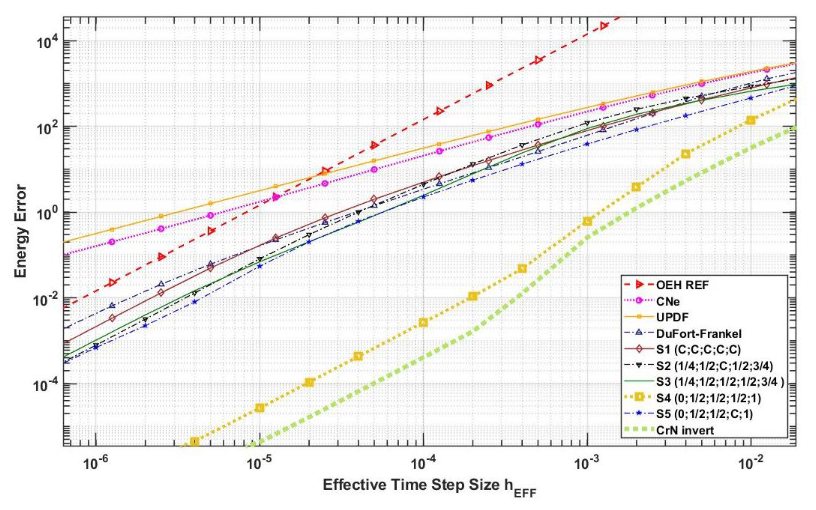
Energy errors as a function of the effective time step size for the first (moderately stiff) system, in the case of the original OEH method (OEH REF), the original one-stage CNe and UPFD method, the new algorithms S1–S5, and the Crank–Nicholson method. For the detailed description of the algorithms, see Section 2 and Section 3.2.
Figure 3.
Energy errors as a function of the effective time step size for the first (moderately stiff) system, in the case of the original OEH method (OEH REF), the original one-stage CNe and UPFD method, the new algorithms S1–S5, and the Crank–Nicholson method. For the detailed description of the algorithms, see Section 2 and Section 3.2.

Figure 4.
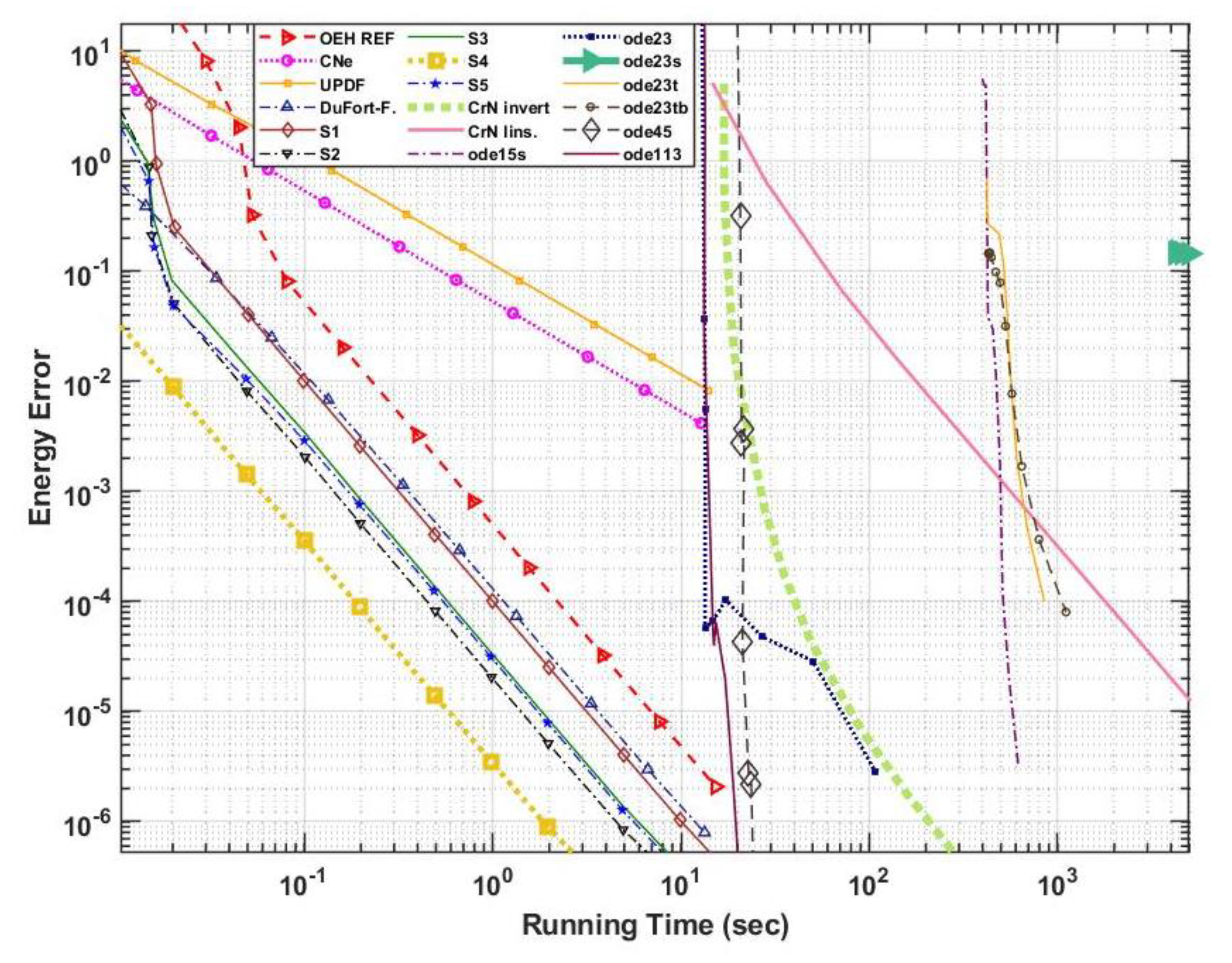
Errors as a function of the running time for the first (moderately stiff) system, in the case of the original OEH method (OEH REF), one-stage CNe and UPFD methods, the Dufort–Frankel method, the new Algorithms S1–S5, and the Crank–Nicolson with two implementations and different MATLAB routines.
Figure 4.
Errors as a function of the running time for the first (moderately stiff) system, in the case of the original OEH method (OEH REF), one-stage CNe and UPFD methods, the Dufort–Frankel method, the new Algorithms S1–S5, and the Crank–Nicolson with two implementations and different MATLAB routines.

Figure 5.
Energy errors as a function of the running time for the first (moderately stiff) system, in the case of the original OEH method (OEH REF), one-stage CNe and UPFD methods, the Dufort–Frankel method, the new Algorithms S1–S5, and the Crank–Nicolson with two implementations and different MATLAB routines.

Figure 6.
Energy errors as a function of the time step size for the second (very stiff) system, in the case of the original OEH method (OEH REF), the original one-stage CNe, UPFD and the Dufort-Frankel methods, the new algorithms S1–S5, and the Crank–Nicholson method.
Figure 6.
Energy errors as a function of the time step size for the second (very stiff) system, in the case of the original OEH method (OEH REF), the original one-stage CNe, UPFD and the Dufort-Frankel methods, the new algorithms S1–S5, and the Crank–Nicholson method.

Figure 7.
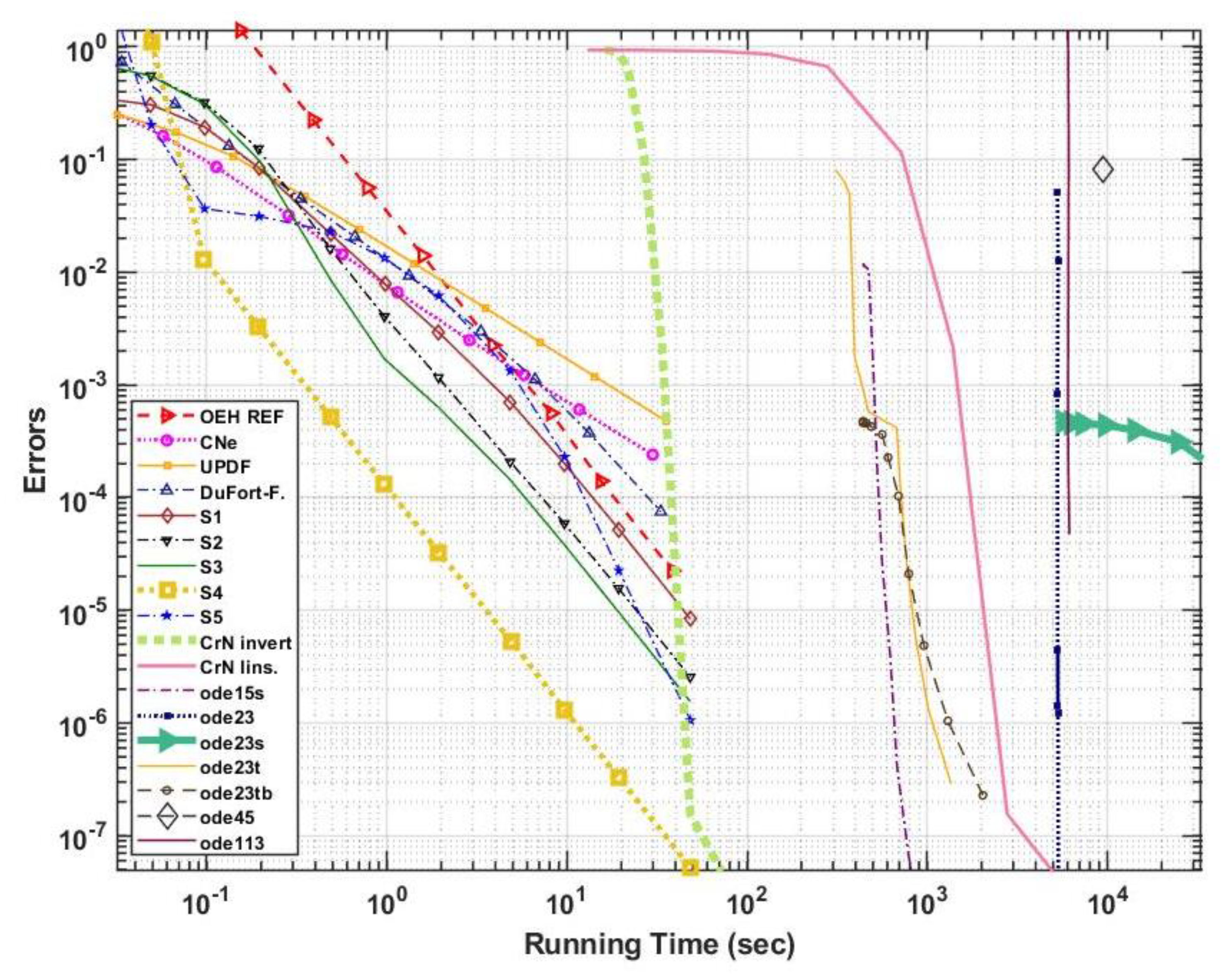
errors as a function of the running time for the second (very stiff) system, in the case of the original OEH method (OEH REF), one-stage CNe and UPFD methods, the Dufort–Frankel method, the new algorithms S1–S5, and the Crank–Nicolson with two implementations and different MATLAB routines.
Figure 7.
errors as a function of the running time for the second (very stiff) system, in the case of the original OEH method (OEH REF), one-stage CNe and UPFD methods, the Dufort–Frankel method, the new algorithms S1–S5, and the Crank–Nicolson with two implementations and different MATLAB routines.

Figure 8.
The errors as a function of for the u2 solutions of the heat equation for .

Figure 9.
The graphs of the second solution, where u0 is the initial function and uref is the analytical solution at the final time, while S3 and S5 are the corresponding numerical solutions served by the S3 (¼, ½, ½, ½, ¾) and the S5 (0, ½, ½, C, 1) algorithms for .
Figure 9.
The graphs of the second solution, where u0 is the initial function and uref is the analytical solution at the final time, while S3 and S5 are the corresponding numerical solutions served by the S3 (¼, ½, ½, ½, ¾) and the S5 (0, ½, ½, C, 1) algorithms for .

Figure 10.
The errors as a function of for the numerical solutions of Fisher’s equation for and .

Figure 11.
The graphs of the eigenvalues of H vs. mesh ratio functions for the S4 (0, ½, ½, ½, 1) algorithm for N = 20. (a) (b) .
Figure 11.
The graphs of the eigenvalues of H vs. mesh ratio functions for the S4 (0, ½, ½, ½, 1) algorithm for N = 20. (a) (b) .


Table 1.
Comparison of different algorithms for the moderately stiff system of 10,000 cells.
| Numerical Method | Running Time (s) | |||
|---|---|---|---|---|
| ode15s, | ||||
| ode23s, | ||||
| ode23t, | ||||
| ode23tb, | ||||
| ode45, | ||||
| ode23, | ||||
| ode113, | ||||
| S1, | ||||
| S2, | ||||
| S3, | ||||
| S4, | ||||
| S5, | ||||
| CrN inv | ||||
| CrN lins |
Table 2.
Comparison of different algorithms for the very stiff system of 10,000 cells.
| Numerical Method | Running Time (s) | |||
|---|---|---|---|---|
| ode15s, | ||||
| ode23s, | ||||
| ode23t, | ||||
| ode23tb, | ||||
| ode45, | ||||
| ode23, | ||||
| ode113, | ||||
| S1, | ||||
| S2, | ||||
| S3, | ||||
| S4, | ||||
| S5, | ||||
| CrN inv | ||||
| CrN lins |
Publisher’s Note: MDPI stays neutral with regard to jurisdictional claims in published maps and institutional affiliations. |
© 2021 by the authors. Licensee MDPI, Basel, Switzerland. This article is an open access article distributed under the terms and conditions of the Creative Commons Attribution (CC BY) license (https://creativecommons.org/licenses/by/4.0/).
Share and Cite
MDPI and ACS Style
Nagy, Á.; Saleh, M.; Omle, I.; Kareem, H.; Kovács, E. New Stable, Explicit, Shifted-Hopscotch Algorithms for the Heat Equation. Math. Comput. Appl. 2021, 26, 61. https://doi.org/10.3390/mca26030061
AMA Style
Nagy Á, Saleh M, Omle I, Kareem H, Kovács E. New Stable, Explicit, Shifted-Hopscotch Algorithms for the Heat Equation. Mathematical and Computational Applications. 2021; 26(3):61. https://doi.org/10.3390/mca26030061
Chicago/Turabian StyleNagy, Ádám, Mahmoud Saleh, Issa Omle, Humam Kareem, and Endre Kovács. 2021. "New Stable, Explicit, Shifted-Hopscotch Algorithms for the Heat Equation" Mathematical and Computational Applications 26, no. 3: 61. https://doi.org/10.3390/mca26030061