Statistical Techniques for Environmental Sciences: A Review

Abstract

This paper reviews the interdisciplinary collaboration between Environmental Sciences and Statistics. The usage of statistical methods as a problem-solving tool for handling environmental problems is the key element of this approach. This paper enhances a clear pavement for environmental scientists as well as quantitative researchers for their further collaborative learning with an analytical base.

1. Introduction

In its simplest sense, the environment means the surrounding external conditions influencing the growth of people, animals or plants, living or working conditions, etc. Environmental Sciences (EVS) is an integrated multidisciplinary approach that studies the environment and solutions of environmental problems. In the present scenario, the environment has become a global agenda item, which has increased the scope and importance of EVS. In the development of different stages of civilization, humans were accompanied both by the environment and statistics. Since the early days, they were found to be knowingly accustomed to the environment and unknowingly played with statistics. Thus, both statistics and the environment have shared a long history of mutual reciprocation. In modern times, these two subjects are independently able to attract the academic attention of scholars throughout the world (see [1]).

The United Nations Statistics Division (UNSD) has an exclusive branch for environmental statistics, established in 1995. Its major area of work is data collection, methodology, capacity development, and coordination of environmental statistics and indicators. They have a dedicated newsletter called “ENVSTATS”, which publishes the activities of UNSD in the area of environmental statistics. The Framework for the Development of Environmental Statistics (FDES 2013) is an updated version of the original FDES, which was published by UNSD in 1984. In India, the Ministry of Statistics and Programme Implementation has a specific publication report in the branch of environmental statistics called “EnviStats” which updates recent developments in the field of environmental statistics.

The extensive use of statistics in EVS led to the development of a new branch called Environmental Statistics. We all know that statistics are an inevitable context in any scientific arena. Even so, the motivation for conducting this specific review is that environmental statistics have an integrated multidisciplinary face, which will shed light on the pure biological field of modern science with its analytical nature. That undiscovered interconnection with statistics and environmental science will be revealed through this review, which will be an easy access point for future investigators. This review has been conducted in two parts, i.e., the pure statistical techniques and those specific techniques that have been exclusively invented for environmental science. A brief state of the art is presented below. The authors of [2] discussed different statistical techniques which are helpful to environmental engineers. It addresses different environmental problems with a solution-oriented approach that encourages students to view statistics as a problem-solving tool.

The use of statistical techniques to understand various environmental phenomena was explained in [3]. He examined different statistical tools, such as probabilistic and stochastic models, data collection, data analysis, inferential statistics, etc. In addition, he discussed principles and methods applicable to a wide range of environmental issues (including pollution, conservation, management, control, standards, sampling, monitoring, etc.) across all fields of interest and concern (including air and water quality, forestry, radiation, climate, food, noise, soil condition, fisheries and environmental standards). Accordingly, he considered sophisticated statistical techniques, such as extreme processes, stimulus response methodology, linear and generalized linear models, sampling principles and methods, time series, spatial models, multivariate techniques, design of experiments, etc.

This article is an attempt to describe some basic statistical concepts used in EVS, thereby establishing a link between the two subjects. It studies some basic statistical concepts relevant to environmental study. Illustrations are discussed on the basis of [4,5].

In this article, Section 2 presents the basic concepts in statistics, Section 3 describes the application of statistical tools in EVS, Section 4 is about the various illustrations regarding the topic, and Section 5 is the conclusion.

2. Basic Concepts

With the advent of the theory of probability and games of chance in the mid-seventeenth century, the concept of modern statistics was born. The name “statistics” appears to have come from the German word “Statistik,” the Italian word “statista,” or the Latin word “status,” all of which mean “political state” or “state craft”, respectively. The term statistics can be used in two different senses.

In the plural sense, it means “a collection of numerical facts”. According to Horace Secrist, “Statistics may be defined as the aggregate of facts, affected to a marked extent by a multiplicity of causes, numerically expressed, enumerated or estimated according to a reasonable standard of accuracy, collected in a systematic manner, for a predetermined purpose and placed in relation to each other”. This definition explains the characteristics of statistical data.

In its singular sense, it means “statistical methods for dealing with numerical data”. According to Croxton and Cowden, “Statistics is the science of collection, presentation, analysis, and interpretation of numerical data”. This definition points out different stages of statistical investigation. Hence, statistics is concerned with exploring, summarizing, and making inferences about the state of complex systems, for example, the state of a nation (social statistics), the state of people’s health (medical and health statistics), the state of the environment (environmental statistics), as extensively described in [6].

In the midst of its wide range of applications and advantages, one important allegation about statistics is that the concerned parties may make misleading statements in their favor. However, the fact is that, as in the case of any science, only an expert can make use of statistical tools effectively. One should make sure that the statistical study is conducted by the right person. There are lots of good ways, many more bad and wrong ways too. So, be sure about the correctness of the tool used. The notorious allegation by Mark Twain citing the British Prime Minister Benjamin Disraeli that “there are three types of lies: lies, damned lies, and statistics” (but the phrase is nowhere in Disraeli’s works, and the earliest known appearances were years after his death, so it is assumed to be by some anonymous writer in mid-1891) is just a lie, provided the precaution is served. In such a context, it is interesting that the author of [7] beautifully coined the title “Truth, Damn Truth and Statistics” for his article.

3. Application of Statistical Tools in EVS

In statistics, data analysis is divided into two sections: descriptive statistics and inferential statistics. The authors of [5] discussed the two in depth, and Section 3.1 and Section 3.2 below present them in summary form.

3.1. Descriptive Statistics

Descriptive statistics are the initial stage of data analysis where exploration, visualization and summarization of data are done. We will look at the definitions of population and random sample in this section. Different types of data, viz. quantitative or qualitative, discrete or continuous, are helpful for studying the features of the data distribution, patterns, and associations. The frequency tables, bar charts, pie diagrams, histograms, etc., represent the data distribution, position, spread and shape efficiently. This descriptive statistical approach is useful for interpreting the information contained in the data and, hence, for drawing conclusions.

Further, different measures of central tendency viz. mean, median, etc., were calculated for analyzing environmental data. It is also useful to study dispersion measures, such as range, standard deviation, etc., to measure variability in small samples. One of the important measures of relative dispersion is the coefficient of variation, and it is useful for comparing the variability of data with different units. Skewness and kurtosis characterize the shape of the sample distribution. The concepts of association and correlation demonstrate the relationships between variables and are useful tools for a clear understanding of linear and non-linear relationships. Important measures of these fundamental characteristics are briefly discussed here in the following.

3.1.1. Central Tendency

The tendency of the observations to cluster around some central value is called central tendency. Any measure of central tendency is termed “average”. The most commonly used averages are the following:

$$\begin{array}{c}\hfill \mathrm{Mean}\overline{x}=\sum _{i=1}^n\frac{x_i}{n},\end{array}$$

where $x_i$ denotes the ith observation and n is the number of observations.

$$\begin{array}{c}\mathrm{Median}\mathrm{is}\mathrm{the}\mathrm{middle}-\mathrm{most}\mathrm{observation}\mathrm{when}\mathrm{observations}\mathrm{are}\mathrm{arranged}\mathrm{in}\mathrm{ascending}\mathrm{or}\hfill \\ \mathrm{descending}\mathrm{order}\hfill \end{array}$$

and

$$\mathrm{Mode}\mathrm{is}\mathrm{the}\mathrm{most}\mathrm{frequently}\mathrm{occurring}\mathrm{observation}.$$

3.1.2. Dispersion

The scattering of observations about the central value is called dispersion. Important measures of dispersion are range, quartile deviation, mean deviation, standard deviation and coefficient of variation. These four measures depend on the unit of measurement of the observations, hence, they are absolute measures. They can be defined as:

$$\mathrm{Range}\mathrm{is}\mathrm{the}\mathrm{difference}\mathrm{between}\mathrm{largest}\mathrm{and}\mathrm{smallest}\mathrm{observations}.$$

Measure based on quartiles:

• Quartile deviation

  $$\begin{array}{c}\hfill QD=\frac{Q_3-Q_2}{2}\end{array}$$

  where $Q_3$ and $Q_2$ are the third and first quartile in the frequency distribution, respectively;
• Mean deviation

  $$\begin{array}{c}\hfill MD=\sum _{i=1}^n\frac{|x_i-\overline{x}|}{n}\end{array}$$

  where $\overline{x}$ is mean of $x_i$ (observed values);
• Standard deviation

  $$\begin{array}{c}\hfill SD=\sqrt{\sum _{i=1}^n\frac{{(x_i-\overline{x})}^2}{n}};\end{array}$$
• Coefficient of variation

  $$\begin{array}{c}\hfill CV=\frac{SD}{\mathrm{Mean}}\times 100.\end{array}$$
  Thus, CV is the relative measure (measure independent of unit) corresponding to SD.

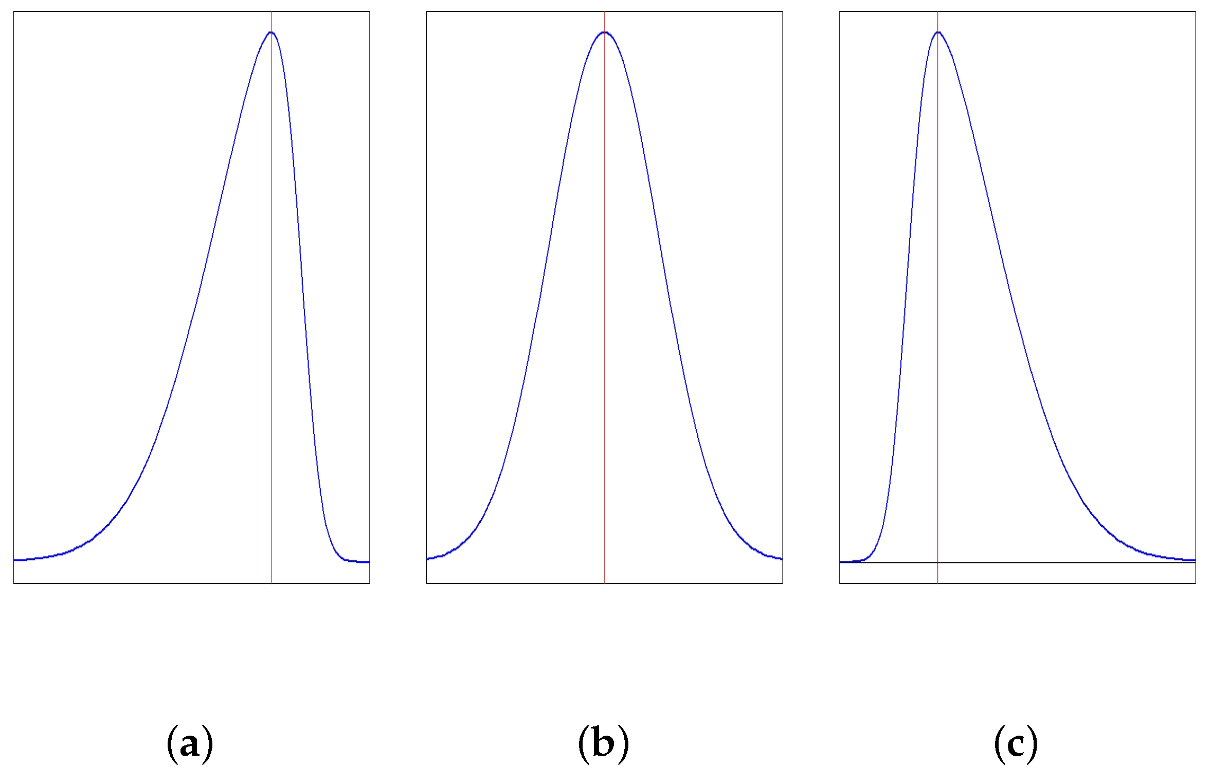
3.1.3. Skewness

The lack of symmetry is termed as skewness or asymmetry. In a frequency curve, if both the sides of the mode are distributed in the same manner, the distribution is symmetric, otherwise it is skewed. When more area is on the right side of the mode, the distribution is positively skewed. If more area is on the left side of the mode, the distribution is negatively skewed. Figure 1 depicts the three situations. There are mainly two measures:

• Pearson’s measure

  $$\begin{array}{c}\hfill S=\frac{\mathrm{Mean}-\mathrm{Mode}}{SD}\end{array}$$
  If $S=0$, the distribution is symmetric, if $S>0$, positively skewed and if $S<0$, negatively skewed.
• Moment measure

  $$\begin{array}{c}\hfill {\beta }_1=\frac{{\mu }_3}{{\mu }_2^{3/2}}\end{array}$$

  where

  $$\begin{array}{c}\hfill {\mu }_2=S{D}^2\end{array}$$

  and

  $$\begin{array}{c}\hfill {\mu }_3=\sum _{i=1}^n\frac{(x_i-\overline{x}{)}^3}{n}.\end{array}$$
  If ${\beta }_1=0$, it is symmetric, if ${\beta }_1>0$, positively skewed and if ${\beta }_1<0$, negatively skewed.

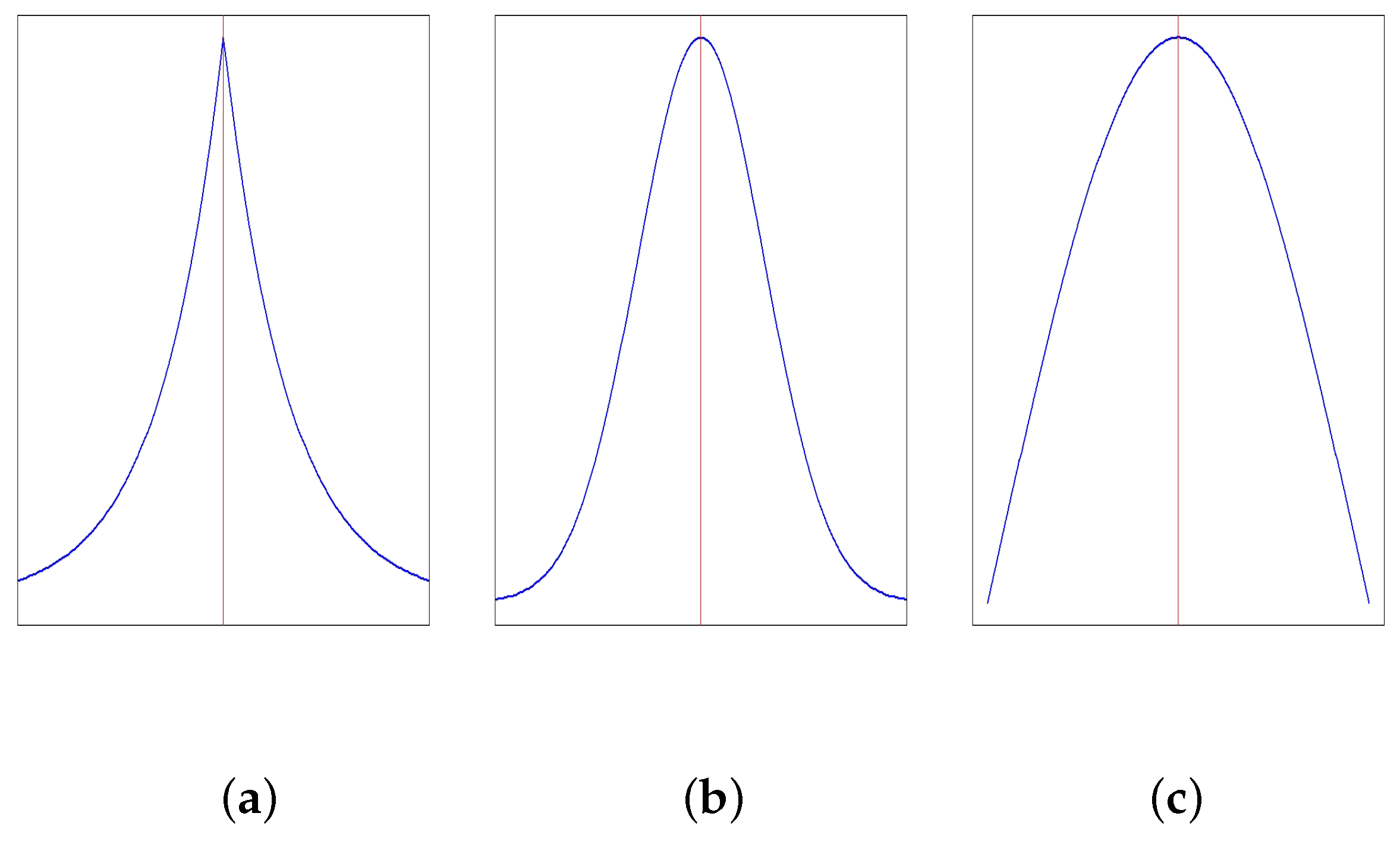
3.1.4. Kurtosis

Kurtosis measures the degree of peakedness or flatness of a curve. The normal curve is called mesokurtic. If the curve is more peaked than normal, it is called leptokurtic. If it is flatter than normal, it is called platykurtic. Figure 2 illustrates the nature of different types of kurtosis.

The moment measure of kurtosis is

$$\begin{array}{c}\hfill {\beta }_2=\frac{{\mu }_4}{{\mu }_2^2}\end{array}$$

where

$$\begin{array}{c}\hfill {\mu }_4=\sum _{i=1}^n\frac{{(x_i-\overline{x})}^4}{n}\end{array}$$

If ${\beta }_2=3$, the distribution is mesokurtic, if ${\beta }_2>3$, the distribution is leptokurtic, and if ${\beta }_2<3$, the distribution is platykurtic.

3.2. Inferential Statistics

In inferential statistics, the concept of probability is important for studying the uncertainties in the environment. For example, whether it will rain or not tomorrow can be best inferred by using probability. Several theoretical probability distributions, such as the Bernoulli distribution, the binomial distribution, the Poisson distribution, etc., are useful for modeling the probability distribution of real environmental data. For example, decisions, such as coin tossing, rain/no rain, yes/no, etc., are explained by Bernoulli variables since their outcomes are binary. In addition, if we are interested in counting the number of times floods occurred in the Dhemaji district of Assam, India, out of the total number of floods that occurred, because we are counting the number of times a flood (X), a Bernoulli event, occurs with a probability of p out of a total, i.e., out of n trials, the probability distribution of such variables is given by a binomial distribution. In addition, if we do not know the total number of flood occurrences but know the meaning of the flood occurrences, the distribution is modeled by the Poisson distribution. Statistical tools such as estimation, hypothesis testing, etc., play a vital role in analyzing environmental data. Some of the frequently used statistical tests in atmospheric and environmental science are the “Z-test,” “T-test,” “F-test,” etc. Another statistical approach is time series analysis, which studies environmental quantities with respect to time. For example, the monthly/yearly mean temperature, rainfall, humidity, etc., are best studied by time series (see [8]).

4. Illustrations

In this section, we are discussing the available statistical techniques that are used in the field of environmental sciences along with some practical examples in the context of data based on environmental sciences. There are examples of how collaboration between environmental scientists and quantitative researchers has aided future learning in both fields, based primarily on two works: [4], which deals with statistical techniques, and [5], which deals with practical examples.

The statistical techniques available are given below, based on [4].

4.1. Methods of Plotting Species Abundance Data

4.1.1. Whittaker Plot

One of the best informative methods is the rank/abundance plot, or dominance diversity curve. Here, species are plotted from most to least abundant along the x axis and abundance in the y axis in ${log}_{10}$ format (here, abundance of several orders of magnitude can be accommodated in the same graph). Proportional or percentage abundance are used in order to facilitate easy comparison.

The authors of [9] named this plot the Whittaker plot in remembrance of R. H. Whittaker for his famous contribution described in [10]. This plot has several advantages. Contrasting patterns of species richness are clearly displayed. If there are only a few of some species, all the information concerning their relative abundance is visible, as they are represented in their histogram format (see [11]). For following environmental impacts and succession, this plot is very effective. For that, we should plot a rank/abundance graph. The shape of the curve gives inference about which species abundance model best fits the data. The steep plot describes assemblages with high dominance, while the shallower plot symbolizes low dominance. High dominance plots are consistent with geometric or log series, while low dominance plots suit the log normal or broken stick model. However, the curves of different models are rarely fitted with empirical data (see [11]).

4.1.2. k-Dominance Plot

This kind of plot shows the relationship between percentage cumulative abundance (y axis) and species rank/log series rank (x axis). Here, the elevated curve represents the less diverse assemblages (see [12,13]).

4.1.3. Abundance/Biomass Comparison Curve or ABC Curve

A variant of the k-dominance plot was introduced by [14]. The related curve is constructed using two measures of abundance: the number of individuals and biomass. The level of disturbance, pollution-induced or otherwise, affecting the assemblage can be inferred from the resulting curve.

The method was developed for benthic macrofauna and has been used productively by a number of investigators in this context.

The ABC plot is used to study the entire species abundance distribution. The author of [15] has introduced a summary statistic specified as W (named after R. M. Warwick), and defined by

$$\begin{array}{c}\hfill W=\sum _{i=1}^S\frac{B_i-A_i}{50(S-1)}\end{array}$$

where $B_i$ denotes the biomass value of each species rank (i) in the ABC curve, S represents the number of species, and $A_i$ represents the abundance (individuals) value of each species rank (i). $A_i$ and $B_i$ do not necessarily refer to the same species, since species are ranked separately for each abundance measure. The result will be positive if the biomass curve is consistently above the individual curve. This symbolizes undisturbed abundance. In contrast, a grossly perturbed assemblage will give a negative value (consistently above the biomass curve). A curve that produces a value of W close to 0 and overlaps signifies moderate disturbance. W ranges usually from $-1$ to +1.

The W statistics are generally computed for each sample separately. ANOVA can be used to test for significant differences, if treatments have been replicated. Alternatively, graphing W values can be a very effective way of illustrating shifts in the composition of the assemblage if un-replicated samples have been taken along a transect or over a time series (such as before, during and after a pollution event). While considering ABC curves at discriminating samples, W statistics are most useful (see [16]).

4.2. Species Abundance Models

Statistical models were initially devised as the best empirical fits to the observed data (see [17]). They help the investigator to objectively compare different assemblages, which is one of its advantages. In some cases, a parameter of the distribution can be used as an index of diversity. Another set of models is biological or theoretical models.

4.2.1. Statistical Models

• log series model
  In this model, the number of species (y axis) is displayed in relation to the number of individuals per species (x axis), the abundance classes which are presented on log scale. This plot is typically used when the log normal distribution is chosen. This type of graph is sometimes dubbed the “Preston plot” (see [18]) in remembrance of Preston F., who pioneered the use of the log normal model in [19]. In the log series model, the mode will fall to the class with the lowest abundance, which represents a single individual, and in the case of this plot, it is more focused on rare species. In log transformation, the x axis has a tendency to shift a mode to the right so as to reveal a log normal pattern.
• Negative binomial model
  The author of [20] describes many applications of the negative binomial model in ecology. Particularly in estimating species richness (see [21]). However, the authors of [22] remarked that it is only rarely fitted to data of species abundance (one exception being [23]). Since it came from a stable log series model, it has some potential interest.
• Zipf-Mandelbrot model
  This model has its roots in linguistics and information theory. This model has several applications in environmental diversity, which are well described in [24,25,26,27,28]. The Zipf-Mandelbrot model is important for a rigorous sequence of colonists from the same species, always present at the same point in the succession in identical habitats. According to [29], this model is not better than the log series or log normal model. This model, however, has been successfully used in [28,30,31,32]. We also refer to [33,34,35] for the use of this model in terrestrial studies, and [36] for the use of this model in aquatic systems. The author of [37] states that it can be used to test the performance of various diversity estimators. The Zipf-Mandelbrot model provided the best description of the cover data, while the biomass data are compatible with the log normal distribution.

4.2.2. Goodness of Fit Tests

A goodness of fit test, often called ${\chi }^2$, is used to find the relationship between the observed and expected frequencies of a species in each abundance class [38]. To fit a deterministic model, the conventional method used is to assign the observed data to abundance classes. Classes based on ${log}_2$ are usually used. According to the model used, the number of species expected in each abundance class is determined.

The model takes the S (number of species) as observed values and N (total abundance), and then determines how these N individuals should be distributed among the S species. If $p<0.05$ (p-value), the model is rejected because it does not adequately describe the pattern of species abundances. If $p>0.05$, the fit fails to be rejected or, ideally, $p>>0.05$ is assumed to be a good fit. Tests of empirical data typically involve a very small number of abundance classes (10 or fewer). This causes a reduction in the degrees of freedom (d.f.) available. The more the degrees of freedom get the least value, the harder it becomes to reject a model.

The authors of [29] remarked that goodness of fit tests work most effectively with large assemblages (but might not be ecologically coherent units). Instead of ${\chi }^2$ he recommends the Kolmogorov–Smirnov (K–S) goodness of fit ($GOF$) test, as said in [38,39]. Indeed, Tokeshi suggests adopting the K–S-$GOF$ test, as the standard method of assessing the goodness of fit of deterministic models. He also suggests the K–S two-sample test can be used to compare two datasets directly to describe their abundance patterns.

The author of [11] reinforces that, if one model fits the data and another does not, it is not possible to conclude that the fit of the two is significantly different. His solution is to use replicated observations. The deviations can be log transformed, if necessary to achieve normality. A multiple comparison test, for example, Duncan’s new multiple range test (see [38]) can then be used to infer which models are significantly different from one another.

4.2.3. Biological or Theoretical Models

• Deterministic and stochastic models
  Deterministic models assume that N individuals will be distributed amongst the S species in the assemblage. The geometric series is the only deterministic niche apportionment model. Stochastic models recognize that replicate communities structured according to the same set of rules will vary according to the relative abundances of species found there, and they try to capture the random elements inherent in natural processes. This makes biological sense. Perhaps not surprisingly, stochastic models are more challenging to fit than their deterministic counterparts. In a practical sense, it is necessary to know whether a model is deterministic or stochastic. Stochastic models have a complexity that requires replicated data, and this problem is solved in Tokeshi’s refinements (see [40]).
• Geometric series
  Assume that the dominant species pre-empts a limiting resource percentage k, and the second most dominant species pre-empts the same k of the remaining part, and so on, until all S have been chosen. If the species abundance is proportional to the resource amount and the assumption stated above is fulfilled, the resulting pattern will follow a geometric series (or niche pre-emption hypothesis). Here, species abundance is ranked from most to least. Ratio of abundance of each species to abundance of predecessor is being a constant through the species and the ranked list is the reason. In addition, the series will appear as a straight line when plotted on log abundance/species rank graph. This plot helps identify whether the dataset is consistent or not with a geometric series. A full mathematical treatment of the geometric series can be found in [41], who also presents the species abundance distribution corresponding to the rank/abundance series. In a geometric series, the abundances of species, ranked from the most to least abundant will be (see [41,42]):

  $$\begin{array}{c}\hfill n_i=N{C}_{k}k{(1-k)}^{i-1}\end{array}$$

  where $n_i$ is the total number of individuals in the ith species, n is the total number of species, N is total number of individuals, k is the proportion of the remaining niche space occupied by each successively colonizing species (k is a constant), and $C_k={\left[1-{(1-k)}^S\right]}^{-1}$ is a constant that insures that ${\sum }_{i=1}^n{n}_i=N$. Because the ratio of the abundance of each species to the abundance of its predecessor is constant through the ranked list of species, the series will appear as a straight line when plotted on a log abundance/species rank graph.
• Broken stick model
  The broken stick model, alias the random niche boundary hypothesis, was proposed in [43]. This model plots relative species abundance in the y axis on a linear scale, and in the x axis, they plot the logged species sequence abundance, so as to represent it from most to least. Then, we will get a straight line. As [22] states, the model has a demerit in that it may be derived from more than one hypothesis. It provides evidence that some ecological factors are being shared more or less evenly between species (see [41]). It represents a group of S species with equal competitive ability vying for niche space, according to [29]. It is typically organized in the order of rank order abundance (see [11]). The authors of [44] prepared a program which estimates species abundance. This model is tricky enough to fit with empirical data (see [29]).
• Tokeshi’s models
  Tokeshi has developed several niche apportionment models, including the dominance pre-emption, random fraction, power fraction, MacArthur fraction, and dominance decay models in [45,46]. They work with the assumption that abundance is proportional to the fraction of niche space occupied by a species. The model here assumes that the target niche selected is divided at random. The only difference between the models is how the target niche is selected. The larger the niche is, the more even the resulting species abundance distribution will be. Evenness ranges from least to most from the dominance pre-emption model, following the order of explanation. The random assortment model represents a random collection of niches of arbitrary sizes (see [45]).

  –

  Random fraction

  In this model, available niche space is divided at random into two pieces. Among these two, one is selected randomly for further subdivision, and so on, till all species are accommodated (see [40]). The sequential breakage model depicts a situation in which a new colonist competes for the niche of a species that is already in the community and takes over a random proportion of the previously existing niche. This model can be used to cover speciation events (see [40]). In addition, this is conceptually simple and found to be fit for a small community of freshwater chironomids (see [45,47]). The authors of [44] have created a Microsoft Excel program which can model the species abundance and distribution associated with it.

  –

  Power fraction model

  The Tokeshi model is applicable to species-rich assemblages, which is an exception to others (see [46]). In this case, the niche space is subdivided in the same way that a random fraction is. However, the probability of a niche splitting increases in this model, albeit only slightly in relation to size (x) via the power function (K). When K approaches 1, the largest niche is selected for fragmentation. When $K=1$, the power fraction model resembles the MacArthur fraction model. Instead, when $K=0$, niche fragmentation is done by random choice and becomes a random fraction model. Usually K is set to 0.5 for the power fraction model (see [46]). Tokeshi accounts for virtually all assemblages. The author of [48] states that larger niches have a high fragmented probability or could occur either ecologically or evolutionarily.

  –

  Dominance pre-emption model

  This model assumes that each species pre-empts more than half the niche space remaining. Because of this, it is dominant among combined species (see [45]). The proportion of available niche space is assigned between 0.5 and 1. When the number of replications increases (or $K=0.75$, the same as the power fraction model), it becomes more similar to the geometric series (see [45]). It can also be applied to niche fragmentation (see [29,40]).

  –

  MacArthur fraction model

  In the case of predicted species abundance distribution, the MacArthur fraction and the broken stick models paved the way to the same result. In this model, the probability of niche fragmentation is inversely proportional to size. This creates a very uniform distribution of species abundances and is only plausible in small communities of taxonomically related species. However, Tokeshi also reminds us that unreplicated data are not good for either the broken stick or the MacArthur fraction models.

  –

  Dominance decay model

  Here, a more uniform pattern of species abundance is considered. At random, the niche space for fragmentation is selected at random. No empirical data indicate that communities as predicted by Tokeshi’s dominance decay model can be found in nature till date. This can be due to insufficient investigations or due to the lower chance of finding an even distribution in nature.

4.2.4. Fitting Niche Apportionment Models to Empirical Data

The author of [45] found a new way of testing stochastic models. Species (S) are listed in decreasing order of abundance. The equation given below is used to fit a niche apportionment model if the mean observed abundance falls within the confidence limits of expected abundance.

$$\begin{array}{c}\hfill R\left(x_i\right)={\mu }_i\pm r{\sigma }_i\sqrt{n}\end{array}$$

where

• $x_{i=1}$ = mean abundance of most abundant;
• $x_{i=2}$ = mean abundance of next most abundant;
• .
• .
• .
• $x_{i=S}$ = mean abundance of least abundant;
• ${\mu }_i$ = mean of abundance ranked from $i=1$ to S;
• ${\sigma }_i$ = standard deviation of abundance;
• n = number of replicated samples;
• r = breadth of confidence limit.

The mean abundance constitutes the observed distribution. For an assemblage of the same number of species (S), the expected abundance is estimated. For this model, we have to choose a large N, ${\mu }_i$, ${\sigma }_i$ and n. In addition, confidence limits are assigned to each rank of expected abundance by considering n rather than N (the number of times the model was simulated).

4.3. Species Richness Indices

There are two well-known species richness indices, which are easy to calculate too, which were introduced by [49,50], respectively.

• Margalef’s diversity index ($D_{Mg}$)

  $$\begin{array}{c}\hfill D_{Mg}=\frac{S-1}{logN}\end{array}$$
• Menhinick’s index ($D_{Mn}$)

$$\begin{array}{c}\hfill D_{Mn}=\frac{S}{\sqrt{N}}\end{array}$$

where S is the number of species recorded, N the total number of individuals in the sample.

Despite the attempt to correct for sample size, both measures remain strongly influenced by sampling effort. Nonetheless, they are intuitively meaningful indices that can be useful in biological diversity research.

Estimating Species Richness

There are two approaches to estimating species richness from samples, as cited in [51,52]. The first is the extrapolation of species accumulation or species–area curves. The second approach is to use a non-parametric estimator.

• Species accumulation curves
  Species accumulation curves, also known as collector curves, plot S, the total number of species, as a function of sampling effort (n) (see [51]). These curves are widely used in botanical research (see [53,54]). This is only a type of species accumulation curve. Curves that are S versus A for different areas (such as islands) and those used in increasingly larger parcels of the same region are the most common.
  The overall shape of species accumulation curves is determined by the order of samples (or individuals). By randomizing, the curve can be made smoother. It also helps deduce the mean and standard deviation of species richness. According to [55], these curves resemble rarefaction curves (see [56]). They usually move from left to right, as new species are added. However, rarefaction curves conventionally move from right to left. Many scientists have plotted species accumulation curves using linear scales on both axes. However, it is better to use a log-transformed x axis since semi-log plots make it easier to identify asymptotic curves from logarithmic curves (see [57]). To find an estimate of total species richness, the authors of [58] extrapolate the graph.
  Functions used in this kind of extrapolation can be classified into asymptotic or non-asymptotic. Both of their roles are to help the user predict an increase in species richness with additional sampling effort rather than to estimate total species richness.

  –

  Asymptotic curves

  They can be generated using two methods. The first is by using a negative exponential model (see [58]). The second is using the Michaelis–Menten equation (see [59]). The usual form of the equation is

  $$\begin{array}{c}\hfill S\left(n\right)=\frac{n{S}_{max}}{B+n}\end{array}$$

  where $S\left(n\right)$ is the number of species observed in n samples, $S_{max}$ is the total number of species in the assemblage, and B is the sampling effort required to detect $50\%$ of $S_{max}$ and n is the sample count.

  –

  Non-asymptotic curves

  These curves are used to estimate species richness. The authors of [60] proposed that the relationship between area and species be best described by a log linear model, extrapolated to a larger area. The authors of [61] imposed an asymptote on the log-log species area curve to avoid extremely high estimates of species richness.

  ∗

  Parametric methods: log series and log normal distributions are the most potent two abundance models in this context (see [51]). Of these, the easiest fit is log series distribution, and it is also simple to apply. In addition, the log series model helps obtain a good estimate of total species richness if the number of individuals in the target area can be estimated. In this case, S will be underestimated where it should not be. Furthermore, this method is also used during rarefaction. Most people adopt the pragmatic approach when fitting continuous log normal distribution, which is inappropriate when observed data are in discrete form (see [22,51]). According to [21], this method has the unique property of generating a mode in the second or third class, giving the appearance of a log normal distribution even if it is not a log normal distribution. There is, however, no method for generating a confidence interval for any estimate of species richness found in a continuous log normal distribution (see [21,22,51,62]). An alternative to this is Poisson log normal (see [51]), which is rarely used as it is hard to fit. However, it produces higher estimates of species richness than any other method.

  ∗

  Non-parametric methods:

  ·

  $Chao1$

  It represents a simple estimator of the absolute number of species in an assemblage, which was introduced by Anne Chao (see [63]). The measure is named by [51] as $Chao1$ and it is based on the number of rare species in a sample. The following notation was provided by [52]:

  $$\begin{array}{c}\hfill S_{Chao1}=S_{obs}+\frac{F_1^2}{2F_2}\end{array}$$

  where $S_{obs}$ denotes the number of species in the sample, $F_1$ is the number of observed species represented by a single individual (singletons) and $F_2$ denotes the number of observed species represented by two individuals (doubletons).

  The requirement for abundance data is an obvious disadvantage of $Chao1$. The abundance data should at least show whether they are singleton or doubleton. However, rather than presence/absence, they are often called incidence or occurrence data. The calculation of the variance of $Chao1$ is possible (see [64,65]).

  ·

  $Chao2$

  Anne Chao was well aware that the number of species found in one sample is the only essential factor for calculation. For this, a new estimator, $Chao2$ was invented. It is as follows (see [51]):

  $$\begin{array}{c}\hfill S_{Chao2}=S_{obs}+\frac{Q_1^2}{2Q_2}\end{array}$$

  where $Q_1$ is the number of species that occur in one sample only (unique species) and $Q_2$ is the number of species that occurs in two samples.

  ·

  Other estimators

  The author of [51] also invented another category of estimator called coverage estimators (see [66]). Coverage estimators are based on the assumption that widespread or abundant species can be included in any sample (see [67]). The abundance-based coverage estimator, alias ACE, is another estimator based on empirical data (see [68]). The partner incidence-based coverage estimator, ICE, focuses its eye on species found in <10 sampling units. Here, to estimate the true number of species, two estimators in this category are Jackknife and bootstrap estimators, which are described in the following sections. The estimators are evaluated using some criteria, such as sample size, patchiness and overall abundance.

4.4. Diversity Measures

Species richness measures and estimators all fall into two categories: either parametric diversity indices or non-parametric diversity indices.

4.4.1. Parametric Measures of Diversity

• log series $\alpha$
  The parameters of the log series model are x and $\alpha$, where $\alpha$ is a diversity index. In addition, $\alpha$ is calculated during the fitting of a distribution. When S and N are known, the value of $\alpha$ can be easily calculated using the Williams monograph (see [69]) or appendix 4 of [70]. Here, x is estimated by iterating the following form:

  $$\begin{array}{c}\hfill \frac{S}{N}=-log(1-x)\frac{1-x}{x}\end{array}$$
  According to [70], until $x⩾0.5$ and as $S>\alpha$, the log series distribution is not the best descriptor of species abundance pattern. In fact, for natural assemblages, usually $x>0.9$ or close to 1 and $S>\alpha$. This implies that $\alpha$ is approximately the same as the number of species represented by a single individual.
• log normal $\lambda$
  The standard deviation ($\sigma$) of the log normal distribution would be a good measure of diversity. Although we can use it as an evenness measure and as an index for discriminating amongst samples, $\sigma$ is not a good choice. It is also impossible to estimate for small sample sizes (see [71]). Then, $S^{*}$ ($S^{*}$ is the estimator of S, the number of species) is a good predictor of total species richness. However, the ratio of these two unsuitable parameters ($S^{*}/\sigma$) turns out to be an effective diversity measure ($\lambda$). It is effective in discriminating against assemblages (see [72]). Its ranking of sites suits well with $\alpha$.
• The Q statistic
  The authors of [73,74] proposed the Q statistic, which is based on the distribution of species abundance data. For this measure, the user does not require a model to fit the empirical data. Hence, for empirical data, a cumulative species abundance curve is drawn and its inter-quartile slope is used to measure diversity. The author of [75] suggests that by restricting the measure to the inter-quartile region, the complete cumulative species abundance curve can be used to explain diversity as well as to remove the bias caused by the extremities (very rare and very abundant species).
  This is analogous to $\alpha$ and hence can be expressed in terms of a log series model, described by [76]. The following equation is estimated from empirical data:

  $$\begin{array}{c}\hfill Q=\frac{(1/2)n_{R_1}+{\sum }_{R_1+1}^{R_2-1}{n}_r+(1/2)n_{R_2}}{log(R_2/R_1)}\end{array}$$

  where $n_r$ is the total number of species with abundance R, $R_1$ and $R_2$ are the 25% and 75% quartiles, $n_{R_1}$ is the number of species in the class where $R_1$ falls, and $n_{R_2}$ is the number of species in the class where $R_2$ falls.
  The quartiles are chosen so that:

  $$\begin{array}{c}\hfill \sum _1^{R_1-1}{n}_r<\frac{1}{4}S\le \sum _1^{R_1}{n}_r\end{array}$$

  and

  $$\begin{array}{c}\hfill \sum _1^{R_2-1}{n}_r<\frac{3}{4}S\le \sum _1^{R_2}{n}_r\end{array}$$

  where S is the total number of species in the sample, although the placement of $R_1$ and $R_2$ is not critical as the inter-quartile region of a cumulative species abundance curve, or indeed a rank/abundance plot, tends to be linear.
  Because $Q=0.371$ for the log normal model, it is not formally a parametric index. Thus, its performance is somewhat similar to that of parametric ones. However, for species which are censused >50%, Q may be biased (see [74]). The author of [77] has found an evenness measure which is similar to Q statistic, i.e., $E_Q$ which will be discussed later.

4.4.2. Non-Parametric Measures of Diversity

Most diversity measures are not explicitly associated with named species abundance models, even though their performance is often governed by the underlying distribution of species abundances. They are non-parametric measures of diversity.

• Shannon Index ($H^{{}^{\prime }}$)
  It was independently derived by Claude Shannon and Warren Weaver and is generally known as the Shannon index or Shannon information index. However, it is sometimes mistakenly referred to as the Shannon–Weaver index (see [9]). It is represented as

  $$\begin{array}{c}\hfill H^{{}^{\prime }}=-\sum _{i=1}^n{p}_{i}log{p}_i\end{array}$$
  Usually, in samples, $p_i$ will be unknown but it is estimated using the maximum likelihood estimator, $n_i/N$ (see [78]), where $n_i$ is the total number of individuals in the ith species and N is the total number of individuals. The ecological validity and computational easiness led Shannon to represent the index as logarithm of $p_i$. Historically, ${log}_2$ is used for calculating the Shannon index, but this is without any biological reason. An increased trend in logarithm standardization is found in [79]. However, Shannon index does not have an unbiased estimate (see [80]).

  –

  A model using Shannon index: Caswell’s neutral model

  Caswell’s neutral model is very famous for its innovative approach to community structure analysis (see [81]). The model focuses on species abundance patterns when biological interactions are removed. It is represented by the deviation statistic defined by

  $$\begin{array}{c}\hfill V=\frac{H^{{}^{\prime }}-E[H^{{}^{\prime }}]}{SD(H^{{}^{\prime }})}\end{array}$$

  where $H^{{}^{\prime }}$ is the Shannon diversity index. It can be used to compare observed diversity ($H^{{}^{\prime }}$) with the predicted neutral diversity $E\left[H^{{}^{\prime }}\right]$. For values of $V>2$ or $V<-2$, it depicts the departure from neutrality [82]. The author of [83] presented a computer program in PRIMER to calculate V which is termed a measure of environmental stress (see [84,85]) but is very rarely used. As richness and evenness are in complex relationships, V is probably useful only as a measure of disturbance. For large values of S and N, the expected values of $H^{{}^{\prime }}$ are generated by a neutral model that closely resembles the predicted values in the log series model (see [70]), where S is the total number of species in the sample and N is the total number of individuals.

• The Shannon evenness measure ($J^{{}^{\prime }}$)
  Assume a situation where all species have equal abundance. Then, the ratio of observed diversity will generate a new measure $J^{{}^{\prime }}$ (see [22,78]). It is defined as

  $$\begin{array}{c}\hfill J^{{}^{\prime }}=\frac{H^{{}^{\prime }}}{H_{max}}=\frac{H^{{}^{\prime }}}{logS}\end{array}$$

  where S is the number of species and $H^{{}^{\prime }}$ is the Shannon diversity index.
  To find $H_{min}$, the author of [86] gives a simple method that can be utilized in other forms of the Shannon evenness (see [87]).
• Heip’s index of evenness ($E_{Heip}$)
  In [88], Heip notes that the evenness measure should not be based on species richness. So, according to this idea, he proposed the following new measure:

  $$\begin{array}{c}\hfill E_{Heip}=\frac{e^{H^{{}^{\prime }}}-1}{S-1}\end{array}$$
  Compared to $J^{{}^{\prime }}$, $E_{Heip}$ is least affected by species richness, it does not require sample size to be independent if there are only 10 species in 1 sample (see [89]). $E_{Heip}$’s minimum value is 0 and it usually goes to 0.006 when an extremely uneven community is considered.
• SHE analysis
  One of the main characteristics of the Shannon index is that it depends extremely on species richness and evenness. In [70,90], they identified that this property of the Shannon index can be utilized in another way. Consider a measure of evenness $E=e^{H^{{}^{\prime }}}/S$ (see [88]), such that

  $$\begin{array}{c}\hfill H^{{}^{\prime }}=logS+logE\end{array}$$
  This decomposition aids the user in interpreting changes in diversity.
  A decrease in diversity tends to cause pollution incidents due to loss of richness, evenness, or a combination of them.
  The essence of SHE analysis is the triangular relationship between S (species richness), H (diversity as measured by the Shannon index) and E (evenness). SHE analysis used by [91] in examining geographic patterns of body mass diversity in Mexican mammals found that evenness was high at intermediate spatial scales but low at the regional one.
• The Brillouin index ($HB$)
  The Brillouin index, abbreviated $HB$, is appropriate when sample randomness is not guaranteed, a community is completely censused, or every individual is accounted for (see [22,78]). It is given as

  $$\begin{array}{c}\hfill HB=\frac{logN!-{\sum }_{i=1}^{S}log{n}_i!}{N}\end{array}$$

  where N is the total number of individuals in the sample, $n_i$ is the number of individuals from the ith species and S is the number of species. The $HB$ value is rarely greater than 4.5. When compared to the Shannon Index, $HB$ always yields a lower value, but they both provide similar or correlated estimates of diversity. The reason is that the Brillouin index describes a completely known collection without any uncertainty.
  Evenness (E) for the Brillouin diversity index is obtained from

  $$\begin{array}{c}\hfill E=\frac{HB}{H{B}_{max}}\end{array}$$

  where $H{B}_{max}$ is calculated as

  $$\begin{array}{c}\hfill H{B}_{max}=\frac{1}{N}log\left(\frac{N!}{N_S{!}^{S-r}(N_S+1){!}^r}\right)\end{array}$$

  where $N_S$ is the integer part of $N/S$ and $r=N-S\left(N_S\right)$.
  The index is unavailable with variance, and hence, no statistical test is needed to test significance. $HB$ is mathematically speaking superior to the other two indices presented by [92]. However, some scientists state that it is more time-consuming and less familiar. Its over-dependence on sample size leads to unexpected results. This is unsuitable when abundance is measured as biomass or productivity (see [9,93]).
• Dominance and evenness measures
  A group of diversity indices is weighted by abundances of the commonest species and is usually referred to as either dominance or evenness measures.

  –

  Simpson’s index (D)

  It is occasionally called the Yule index in remembrance of G. U. Yule (see [20]). The probability of any two individuals drawn at random from an infinitely large community being of the same species is given by [94] as

  $$\begin{array}{c}\hfill D=\sum _{i=1}^n{p}_i^2\end{array}$$

  where $p_i$ denotes the proportion of individuals in the ith species, and n number of species. The form of the index appropriate for a finite community is:

  $$\begin{array}{c}\hfill D=\sum _{i=1}^n\frac{n_i(n_i-1)}{N(N-1)}\end{array}$$

  where $n_i$ is the number of individuals in the ith species and N is the total number of individuals in the sample.

  Simpson’s index is expressed as $1-D$ or $1/D$ because diversity decreases as D increases, and thus, it captures the variance of species abundance distribution. Simpsons’ index, on the other hand, is less sensitive to species richness and more oriented toward species abundance. Confidence limits are applied using jackknifing. Simpson’s index is the most meaningful and robust of all the measures. The reciprocal nature of the Simpson index was questioned by [95] and he recommends using $log\left(D\right)$ instead of $(1-D)$ or $(1/D)$, because this notation ensures severe variance problems. He also advises Kemp’s transformation.

  –

  Simpson’s measure of evenness ($E_{1/D}$)

  The Simpson measure of evenness, denoted by $E_{1/D}$ and stated in [9,89], is defined by

  $$\begin{array}{c}\hfill E_{1/D}=\frac{1/D}{S}\end{array}$$

  Here, $E_{1/D}$ usually ranges between 0 and 1 and is not so related to species richness. Because Simpson’s index is a product of Simpson’s evenness measure and S, multiplying S turns any good evenness index into a heterogeneity measure (see [96]).

  –

  McIntosh’s measure of diversity (U)

  McIntosh postulated in 1967 that a community may be thought of as a point in a S-dimensional hyper volume, with the Euclidean distance between the assemblage and its origin serving as a measure of diversity (see [97]). The distance is known as U and is calculated as

  $$\begin{array}{c}\hfill U=\sqrt{\sum _{i=1}^n{n}_i^2}\end{array}$$

  where $n_i$ is the number of individuals in the ith species and n number of species. The McIntosh U index is formally not a dominance index. However, a measure of diversity (D) or dominance that is independent of N can also be calculated as

  $$\begin{array}{c}\hfill D=\frac{N-U}{N-\sqrt{N}}\end{array}$$

  A further evenness measure can be obtained from the following formula (see [22]):

  $$\begin{array}{c}\hfill E=\frac{N-U}{N-N/\sqrt{S}}\end{array}$$

  –

  The Berger-Parker index (d)

  The Berger-Parker index, denoted by d, is an easy-to-calculate dominance measure (see [41,98]). The proportional abundance of the most abundant species is expressed by this index:

  $$\begin{array}{c}\hfill d=\frac{N_{max}}{N}\end{array}$$

  where $N_{max}$ is the number of individuals in the most abundant species. In this case, d denotes the relative importance of the most dominant species in the assemblage; both are considered equivalent. The reciprocal form of the Berger-Parker index is accepted because an increase in the value of the index accompanies an increase in diversity and a reduction in dominance, making it similar to Simpson’s index. It is one of the most satisfactory diversity measures available because of its simplicity and biological significance (see [41]). In small assemblages, d is independent of S, and its value decreases with increasing species richness.

  –

  Nee, Harvey and Cotgreave’s evenness measure ($E_{NHC}$)

  As an evenness measure, the authors of [77] proposed the slope b of a rank/abundance plot (with abundances log transformed). The resulting measure is

  $$\begin{array}{c}\hfill E_{NHC}=b\end{array}$$

  $E_{NHC}$ ranges from $-\infty$ and 0, where 0 is perfect evenness. This measure is difficult to interpret due to its range of values. It is more properly a measure of diversity than of evenness, and this is one of its demerits (see [73]). The authors of [89] therefore proposed a new form of the measure, which is

  $$\begin{array}{c}\hfill E_Q=-\frac{2}{\pi arctan\left(b^{\prime }\right)}\end{array}$$

  In this measure, the ranks are scaled before the regression is fitted, and $b^{\prime }$ denotes the corresponding slope. Thus, this is accomplished by dividing all ranks by the highest rank, such that the most abundant species receives a rank of 1.0 and the least abundant receives a rank of $1/S$. The transformation ($-2/[\pi arctan\left(b^{\prime }\right)]$) places the measure in the 0 (no evenness) to 1 (perfect evenness) range.

  –

  Camargo’s evenness index ($E_c$)

  The author of [99] also introduced the following evenness measure:

  $$\begin{array}{c}\hfill E_c=1-\sum _{i=1}^S\sum _{j=i+1}^S\frac{p_i-p_j}{S}\end{array}$$

  where $E_c$ is Camargo’s index of evenness, $p_i$ the proportion of species i in the sample, $p_j$ the proportion of species j in the sample, and S the sample size.

  Although, the index is simple to calculate and relatively unaffected by rare species (see [100]). The authors of [37] found it to be biased, especially in comparison with the Simpson index.

  –

  Smith and Wilson’s evenness index ($E_{var}$)

  The authors of [89] proposed a new index to provide an intuitive measure of evenness. This index takes the variation in species abundances and divides it by log abundance to produce proportional differences. This makes the index independent of measurement units. Smith and Wilson called their measure $E_{var}$. It is defined by

  $$\begin{array}{c}\hfill E_{var}=1-\frac{2}{\pi arctan\left\{{\sum }_{i=1}^S{\left(log{n}_i-{\sum }_{j=1}^S\frac{log{n}_j}{S}\right)}^2/S\right\}}\end{array}$$

  where $n_i$ is the number of individuals in species i, $n_j$ is the number of individuals in species j and S represents the total number of species. The conversion by $1-2/(\pi arctan(x\left)\right)$ ensures that the resulting measure falls between 0 (minimum evenness) and 1 (maximum evenness).

4.4.3. Taxonomic Diversity

If two assemblages have the same number of species and similar patterns of species abundance, but differ in the diversity of taxa to which the species belong, it seems intuitively reasonable that the assemblage with the most taxonomically diverse taxa is the more diversified assemblage. A taxonomic distinctness measure is one of the most recent developments in taxonomic diversity (see [101,102]).

• Clarke and Warwick’s taxonomic distinctness index
  This measure gives the average taxonomic distance, or simply the path length between two randomly chosen organisms through phylogeny. Two forms can be taken by species in an assemblage. The first is taxonomic diversity ($\Delta$), which considers taxonomic relatedness or species abundance. The two organisms may belong to the same species. The second form is taxonomic distinctness (${\Delta }^{*}$), a pure measure of taxonomic relatedness, which is equivalent to dividing $\Delta$ by the value it would take if all species belonged to the same genus, that is, in the absence of a taxonomic hierarchy. When presence/absence data are used, both measures reduce to the same statistic, ${\Delta }^{+}$, which is the average taxonomic distance between two randomly selected species. It is calculated as follows:

  $$\begin{array}{c}\hfill {\Delta }^{+}=\frac{{\sum }_{i=1}^S{\sum }_{j=i+1,i<j}^S{\omega }_{ij}}{S(S-1)/2}\end{array}$$

  where S denotes the number of species in the study and ${\omega }_{ij}$ is the taxonomic path length between species i and j.
  The taxonomic distinctness index is distinguished by its lack of reliance on sampling effort (see [103]).
  Using ${\Delta }^{+}$, a significance test can be carried out. Here, the null hypothesis considered is “taxonomic distinctness of a locality is not significantly different from the global list”. On the other hand, the author of [104] used multivariate methods during detection of small variations in community structure and diversity. Multivariate analysis also helps find increased variability between samples (see [105]).

4.5. Sampling: An Essential Attribute

There are essentially two choices regarding sample size. The investigator may either adjust the sample size to cope-up with the situation or adopt a standard sample size. The second approach, which is also recommended by [70], is the best. If two samples with different sample sizes are drawn from the same assemblage, then this may lead to different conclusions about its diversity (see [22]). If samples are replicated several times, the curve obtained by plotting the measure of diversity (or evenness) against cumulative sample size may lead to a smooth curve.

• Replications
  The number of replications required is always an unanswerable question. Ideally, the available sample size and number of replications required to complete this are selected on the basis of the most diverse assemblage. In addition, it will be the same throughout the study. When sample size is not consistent, this becomes more true.
  One should be well aware of the difference between replication and pseudoreplication (see [106]). For more ideas in this context, users can refer to [107]. The primary condition is that all replicates must be independent (spatially).

4.6. Comparison of Communities

The manner in which the statistical comparison of communities or other ecological entities is achieved depends to some extent, though with significant overlaps, on the aspect of biodiversity that has been measured.

• Rarefaction—Sample data to common abundance level
  Rarefaction is a technique that reduces sample data to a common abundance level, which helps direct mapping between species richness in communities. During rarefaction, to estimate the richness of a small sample, complete information regarding all the collected species is required. Rarefaction curves converge when sample sizes are small (see [55,108]). Sampling should be enough to characterize the community, but there is a chance that estimates will be biased if the sample is insufficient.
  The author of [109] states that software can be used to create rarefaction curves. In [65], sample-based rarefaction curves were calculated using the EstimateS software. Confidence intervals can be incorporated into these curves. Rarefaction by the log series model is computationally simple. Indeed, it may even be used in circumstances where species abundances do not follow a log series distribution. However, if the sampling was inadequate in the first place, no method of rarefaction is going to compensate.
• Statistical tests
  Standard statistical techniques such as T-tests and ANOVA can be used to compare assemblages (see [38]). Alternatively, jackknifing or bootstrapping can be used to attach confidence intervals to a diversity statistic.

  –

  Jackknifing: a measure of diversity

  Jackknifing (see [110]) is a strategy for improving the estimate of almost any statistic. It can also be used to calculate the number of species present. It was first proposed by Quenouille in 1956, with Tukey making changes in 1958. The author of [111] was the first to apply the approach to diversity statistics. This application was further investigated by [112,113].

  Jackknifing does not require assumptions about the underlying distribution. Instead, it uses a set of “pseudo-values” which are artificially produced. These pseudo-values are (usually) normally distributed, their mean forms the best estimate of the statistic. Approximate confidence limits can also be attached to the estimate. The procedure is simple. The first step is to estimate the diversity of all n samples together. This produces St, the original diversity estimate. Next, the diversity measure is recalculated n times, missing out each sample in turn. Each recalculation produces a new estimate, $S{t}_{-i}$. The pseudo-value (${\varphi }_i$) can then be calculated for each of the n samples as

  $$\begin{array}{c}\hfill {\varphi }_i=nSt-(n-1)S{t}_{-i}\end{array}$$

  The jackknifed estimate of the diversity statistic is simply the mean of these pseudo-values:

  $$\begin{array}{c}\hfill \overline{\varphi }=\sum _{i=1}^n\frac{{\varphi }_i}{n}\end{array}$$

  The approximate standard error of the jackknifed estimate is

  $$\begin{array}{c}\hfill S{E}_{\overline{\varphi }}=\sqrt{\sum _{i=1}^n\frac{{({\varphi }_i-\overline{\varphi })}^2}{n(n-1)}}\end{array}$$

  This standard error may be used to assign approximate confidence limits to the jackknifed diversity estimate. Confidence limits are set in the usual way, i.e.,

  $$\begin{array}{c}\hfill \overline{\varphi }\pm t_{0.05(n-1)}S{E}_{\overline{\varphi }}\end{array}$$

  Prior to jackknifing, the author of [38] recommended that statistics with a restricted range (such as those constrained between 0 and 1) should be modified. Following that, same methods were used to estimate species richness, with considerable success. They are called Jackknife 1, a first-order jackknife estimator that employs the number of species that occur only in a single sample (see [114,115]), and Jackknife 2, a second-order estimator which, like the $Chao2$ equation, takes both the number of species found in one sample only ($Q_1$) and in precisely two samples ($Q_2$) into account (see [116]). Both require incidence data.

  In the following equations, m denotes the number of samples:

  $$\begin{array}{c}\hfill S_{Jack1}=S_{obs}+Q_1\left(\frac{m-1}{m}\right)\end{array}$$

  $$\begin{array}{c}\hfill S_{Jack2}=S_{obs}+\left(\frac{Q_1(2m-3)}{m}-\frac{Q_2{(m-2)}^2}{m(m-1)}\right)\end{array}$$

  The variances of both estimators can be calculated.

  –

  Bootstrapping

  A related method for producing standard errors and confidence bounds is bootstrapping. It is more computationally intensive than the jackknife, although it is regarded as an improvement. In essence, the original dataset is sampled numerous times to obtain a large number of different observations. These are then used to deduce the standard error. The authors of [20,38] provide more details. Bootstrapping, like jackknifing, can be used in species richness estimation.

• Null models
  In the last decade, there has been a rising use of null models in diversity measurement. Ecologists are becoming aware of the importance of developing testable null hypotheses (see [117]). The observed patterns are not due to the presumed causal explanation, according to the null hypothesis. It is based on the assumption that nothing significant has occurred (see [118]). Null models can also be used to determine whether perceived differences in diversity are simply an artifact of sampling. As [55] emphasizes, a null model does not presume that there is no structure in a community or that all processes are random. Instead, randomness is assumed only in respect of the mechanism being tested. Null models are already used extensively to evaluate species co-occurrence patterns (see [119]).

4.7. Diversity in Space (and Time)

Till now, we have focused on the diversity of a defined assemblage or habitat, or $\alpha$ diversity. The author of [120] makes the distinction between $\alpha$ and $\beta$ diversity where diversity increases as the similarity in species composition decreases. $\beta$ diversity reflects biotic change or species replacement, whereas $\alpha$ diversity is a property of a specific spatial unit. The diversity of two or more spatial units differs. We can use $\beta$ diversity. The relationship between $\alpha$ and $\beta$ diversity is scale-dependent. The observation made by [80] is that

$$\begin{array}{c}\hfill D_{\gamma }={\overline{D}}_{\alpha }+D_{\beta }\end{array}$$

When species richness is used to measure $\alpha$ and $\gamma$ diversity, $\beta$ diversity may be estimated as follows:

$$\begin{array}{c}\hfill D_{\beta }=S_T-\overline{S_j}=\sum _{j=1}^n{q}_j(S_T-S_j)\end{array}$$

where $S_T$ is the species richness of the landscape ($\gamma$ diversity), $S_j$ denotes the richness of assemblage j and $q_j$ is the proportional weight of assemblage j based on its sample size(n) or importance.

This approach is also used in the Shannon and Simpson diversity measurements. Low $\alpha$ and high $\beta$ diversity will come from many small sampling units, but the opposite will be true if there are fewer but larger samples. If all other factors are equal, both sampling procedures yield the same conclusions concerning $\gamma$ diversity.

• Indices of $\beta$ diversity
  The majority of these indices use presence/absence data and, as such, focus on the species richness element of diversity.
  • Whittaker’s measure (${\beta }_W$)
    One of the simplest, and most effective, measures of $\beta$ diversity was devised by [120]:

    $$\begin{array}{c}\hfill {\beta }_W=\frac{S}{\overline{\alpha }}\end{array}$$

    where S is the total number of species recorded in the system (i.e., $\gamma$ diversity) and $\alpha$ is the average sample diversity, where each sample is a standard size and diversity is measured as species richness. This is equivalent to:

    $$\begin{array}{c}\hfill D_{\beta }=\frac{S_T}{\overline{S_j}}\end{array}$$

    in Lande’s notation.
    When Whittaker’s measure is used to compute ${\beta }_W$, values of the measure will range from 1 (complete similarity) to 2 (no overlap in species composition). The author of [121] introduced a modification of Whittaker’s measure. This allows the user to compare two transects (or samples) of different size. The related formula is

    $$\begin{array}{c}\hfill {\beta }_{H1}=\frac{S/\alpha -1}{N-1}\times 100\end{array}$$

    where S denotes the total number of species recorded, $\alpha$ means $\alpha$ diversity and N is the number of sites (or grid squares) along a transect. The measure ranges from 0 (no turnover) to 100 (every sample has a unique set of species) and can be used to examine pairwise differentiation between sites. The author of [121] suggested a second modification which is insensitive to species richness trends. It is given by

    $$\begin{array}{c}\hfill {\beta }_{H2}=\frac{S/\left({\alpha }_{max}-1\right)}{N-1}\times 100\end{array}$$
    Here, ${\alpha }_{max}$ is the maximum within-taxon richness per sample. The authors of [122] used ${\beta }_{H2}$ to compare the turnover of various taxa in relation to disturbance in a Cameroon forest.
  • Cody’s measure (${\beta }_C$)
    The author of [123] proposed an index, which is easy to calculate and is a good measure of species turnover. It is given by

    $$\begin{array}{c}\hfill {\beta }_C=\frac{g\left(H\right)+l\left(H\right)}{2}\end{array}$$

    where $g\left(H\right)$ is the number of species gained and $l\left(H\right)$ is the number of species lost.
  • Routledge’s measures (${\beta }_R,{\beta }_I$ and ${\beta }_E$)
    The author of [124] was concerned with how diversity measures can be partitioned into $\alpha$ and $\beta$ components. His first index, denoted by ${\beta }_R$, takes overall species richness and the degree of species overlap into consideration. This index is defined by

    $$\begin{array}{c}\hfill {\beta }_R=\frac{S^2}{2r+S}-1\end{array}$$

    where S is the total number of species in all samples and r is the number of species pairs with overlapping distributions.
    ${\beta }_I$, the second index, stems from information theory and has been simplified for presence/absence data and equal sample size by [125]:

    $$\begin{array}{c}\hfill {\beta }_I=logT-\frac{1}{T}\sum _{i=1}^n{e}_{i}log{e}_i-\frac{1}{T}\sum _{j=1}^n{S}_{j}log{S}_j\end{array}$$

    where $e_i$ is the number of samples in the transect in which species i is present, $S_j$ is the species richness of sample j, and $T={\sum }_{i=1}^n{e}_i$ = ${\sum }_{i=1}^n{S}_j$, and n the total number of samples.
    The third index, ${\beta }_E$, is simply the exponential form of ${\beta }_I$. That is

    $$\begin{array}{c}\hfill {\beta }_E=e^{{\beta }_I}\end{array}$$
  • Wilson and Shmida’s index ${\beta }_T$
    The authors of [125] proposed a new measure of $\beta$ diversity. It is given by

    $$\begin{array}{c}\hfill {\beta }_T=\frac{g\left(H\right)+l\left(H\right)}{2\overline{S_j}}\end{array}$$

    where $\overline{S_j}$ is the mean of $S_j$. Most measures of $\beta$ diversity are sensitive to scale. Turnover decreases as progressively larger areas are investigated.
• Indices of complementarity and similarity
  The author of [126] coined the term complementarity to characterize the differences across locations in respect of the species they support. Complementarity is, of course, another name for the $\beta$ variety. The larger the $\beta$ diversity of two sites, the more complimentary they are. Measures typically combine three variables: a, the total number of species present in both quadrants or samples, b the number of species present only in quadrant 1 and c the number of species present only in quadrant 2. There are mainly two indices.
  • Marczewski–Steinhaus (MS) distance
    Following [127], the author of [51] recommended the Marczewski–Steinhaus (MS) distance as a measure of complementarity. It is expressed as

    $$\begin{array}{c}\hfill C_{MS}=1-\frac{a}{a+b+c}\end{array}$$
    This measure is in fact the complement of the familiar [128] similarity index:

    $$\begin{array}{c}\hfill C_J=\frac{a}{a+b+c}\end{array}$$
    As suggested by Pielou, the statistic can also be adapted to give a single measure of complementarity across a set of samples or along a transect:

    $$\begin{array}{c}\hfill C_T=\sum _{i=1}^n\sum _{j=1,i\ne j}^n\frac{U_{jk}}{n}\end{array}$$

    where $U_{jk}=S_j+S_k-2V_{jk}$ and is summed across all pairs of samples, $V_{jk}$ is the number of species common to the two lists j and k (the same value as a in the formulae above), $S_j$ and $S_k$ are the number of species in samples j and k, respectively, and n is the number of samples.
    When n is large, $C_T$ approaches a value of $n{S}_T/4$, where $S_T$ is the species richness of all samples combined.
    A metric (as opposed to a nonmetric) measure is the Marczewski–Steinhaus dissimilarity measure (and hence the complement of the Jaccard similarity measure). This indicates that it meets specific geometric criteria. The significant result for the user is that it may now be used as a distance measure and in ordination (see [127]).
  • Sorensen’s measure
    Another popular similarity measure was devised by [129]:

    $$\begin{array}{c}\hfill C_S=\frac{2a}{2a+b+c}\end{array}$$
    Sorensen’s measure (see [20]) is widely recognized as one of the most effective presence/absence similarity metrics. The Bray-Curtis presence/absence coefficient is the same.
  • Lennon turnover measure
    Sorensen’s measure will always be large. Therefore, they introduce a new turnover measure ${\beta }_{sim}$, that focuses more precisely on differences in composition:

    $$\begin{array}{c}\hfill {\beta }_{sim}=1-\frac{a}{a+min(b,c)}\end{array}$$
    This is related to a measure derived by [130]. Any difference in species richness inflates either b or c. The consequence of using the smallest of these values in the denominator is thus to reduce the impact of any imbalance in species richness. The authors of [131] found that this measure performs well.
    One of the primary advantages of these measurements is that they are simple to calculate and comprehend. Furthermore, the coefficients do not take into consideration the relative abundance of species, which is a flaw.
  • Sorensen quantitative index or Bray-Curtis index
    Similarity/dissimilarity measures based on quantitative data. The author of [132] introduced a modified version of the Sorensen index. This is sometimes called the Sorensen quantitative index (see [133]). It is given by

    $$\begin{array}{c}\hfill C_N=\frac{2jN}{N_a+N_b}\end{array}$$

    where $N_a$ is the total number of individuals in site A, $N_b$ is the total number of individuals in site B, and $2jN$ is the sum of the lower of the two abundances for species found in both sites.
  • Other notable indices
    The authors of [134] looked into a number of quantitative similarity indices and discovered that, with the exception of the Morisita–Horn index, they were all heavily influenced by species richness and sample size. The Morisita–Horn index (MH) has the drawback of being extremely sensitive to the abundance of the most abundant species. Despite this, the author of [135] was able to measure $\beta$ diversity in tropical cockroach assemblages using a modified version of the index. It is defined by

    $$\begin{array}{c}\hfill C_{MH}=\frac{2{\sum }_{i=1}^n{a}_i{b}_i}{(d_a+d_b)\times N_a\times N_b}\end{array}$$

    where $N_a$ is the total number of individuals at site A, $N_b$ is the total number of individuals at site B, $a_i$ is the number of individuals in the ith species in A, $b_i$ is the number of individuals in the i species in B, n is the total number of species and $d_a$ and $d_b$ are calculated as follows:

    $$\begin{array}{c}\hfill d_a=\frac{{\sum }_{i=1}^n{a}_i^2}{N_a^2}\end{array}$$
    The Morisita–Horn measure is widely used (see [136,137]). The authors of [20] provided a version of Morisita’s original index that is suitable for easy computation. A further simple measure is percentage similarity (see [20]):

    $$\begin{array}{c}\hfill P=100-0.5\sum _{i=1}^S|P_{ai}-P_{bi}|\end{array}$$

    where $P_{ai}$ and $P_{bi}$ is the percentage abundances of species i in samples a and b, respectively, and S is the total number of species.

Some practical applications are given below based on [5].

4.8. Extreme Values in Modeling Atmospheric Ozone

The traditional method of extreme value analysis popularized by [138] was the annual maximum method, in which one of the three classical types of extreme value distributions was fitted to, say, the annual maxima of a river or sea level series. Modified approaches to extreme value analysis which cope with time series dependence are discussed by [139,140]. The extreme value trend centered on the statistical features of insurance claims for environmental damage. The author of [141] suggested that exceedances over a high threshold can be modeled approximately by the generalized Pareto distribution (GPD).

4.9. Environmental Epidemiology

The study of associations between environmental pollutants and negative health consequences is a prominent topic in current environmental health science.

The authors of [142,143] have considered some methodological issues associated with detecting clusters in spatial point processes of disease. The authors of [144] extended the approach to the modeling of spatially aggregated data. Earlier, the authors of [145] proposed a non-parametric test for identifying disease clusters. However, as there are several sources for a disease, it has become impossible to associate the effect of each. Therefore, the cluster cannot be detected easily. In such cases, it is generally assumed that comparison of mortality or disease incidence with levels of counter-revolutionary spatial regions is subject to so much confounding with other environmental effects. To estimate the sequential mean and covariances, Zidek adapted Bayesian approach on spatial prediction of a multidimensional variable (see [146]).

4.10. Adaptive Sampling for Pollution ‘Hot Spots’

The population mean concentration of the chemical pollutant will be estimated by identifying hotspots. Some clusters may be overlooked if basic random sampling is used. The sample mean, while unbiased as a population mean estimate, will have a substantial variance. In this circumstance, adaptive sampling is a viable alternative. In this case, the sampling procedure’s direction at any stage is influenced at least in part by the information gathered in prior samplings.

The sampling procedure is as follows. Take a random sample of a certain size from the study area. Return and sample every unit adjacent to the contaminated unit if any of the selected units reveals contamination. If any neighboring units exhibit contamination, sample their neighbors, and so on, until each detected cluster has a clean boundary.

The total sample size is unknown in advance, however, the accuracy of the outcome will overcome this disadvantage. However, if the resulting data are evaluated naively, this strategy will produce erroneous estimates of population parameters. To avoid this, the authors of [147] outlined a sampling theory, i.e., employed a useful strategy for selecting the initial sample in clusters and stratifying those samples. Then, using modified Horvitz–Thompson or Hansen–Hurwitz estimators, unbiased estimators of the unknown population’s mean can be obtained. These estimators, such as the mean of the initial sample, are unbiased, but they do not always have the lowest variance. The Rao–Blackwell theorem can be used to improve them.

4.11. Trend Analysis

Analysis of trends in environmental science leads to adjustments for autoregressive effects or other spatial-temporal correlations in the data. This is another important area of environmental trend analysis (see [148]). Any data that posses time-dependency will lead to auto-correlation and then to time series analysis.

4.12. Ecological Modeling

In building stochastic models of vertebrate populations, statistics have an useful interaction with fisheries and wildlife sciences. Analyzing the survival of the northern spotted owl after it experiences habitat loss and employing the well-known Leslie–Lefkovitch model suggested by [149] is an example. The model uses information about survival and fecundity in a matrix framework to predict future age structure based on past age structure information. After statistical analysis, it is found that the characteristic root was significantly less than zero, suggesting a decline in female owl populations due to habitat loss. However, other parameters, including vitality rates, do not show any negative trend. Here, they use an appropriate variance model, which is critical in stochastic modeling.

If single sampling is considered, the variance estimate computed will be misleading. However, if a number of sampling occasions are considered, then the process variance will give a better estimate.

4.13. Combining Environmental Information

Another increasingly important issue in the environmental sciences is the need to combine information from diverse sources that relate to a common endpoint. Combining information is a very active area of statistical and applied subject-matter research.

A common technique for combining independent results is Meta analysis (see [150]), which brings together the results of different studies, reanalyzes the disparate results within the concept of their common endpoints, and provides a quantitative analysis of the phenomenon of interest based on the combined data. In the case of environmental science, the effect of interest may be very small and therefore hard to detect. The limited sample sizes or data on many multiple endpoints lead to highly localized effects.

• Combining p-values: Perhaps, the most known method of combining information is Fisher’s inverse ${\chi }^2$ method (see [151]), where individual p-values, (P${}_k$), from K independent studies are combined. The resultant is combined p-value, which is compared to a ${\chi }^2$ reference distribution with 2K degrees of freedom.
• Hierarchical Bayesian method of combining information which leads to Bayesian or empirical Bayesian analysis.
• Hierarchical regression model: The inclusion of factors that represented the various sources of variability was a key element. The odds ratio of exposure for responding patients (cases) versus non-responding, healthy subjects (controls) was the outcome of interest in each investigation. The hierarchical model was able to synthesize information across the ensemble of data, allowing more significant impacts to be investigated.

4.14. Space–Time Modeling with Applications to Atmospheric Pollution and Acid Rain

The space time autoregressive moving average (STARMA) approach was utilized by [152] (see [153]). For most latitudes, Niu and Tiao chose the STAR(2,1) model. The authors of [154] studied the logarithms of sulfate content in rainfall at 19 sites in the eastern and mid-western United States for 24 monthly measurements from 1982 to 1983, and came up with a substantially different atmospheric contaminant model. They calculated their estimator’s variance. An empirical Bayesian approach was used to generate the sample spatial covariance matrix from the residuals of the fit.

4.15. Detection Limits

The authors of [155] illustrated a robust parametric method for quantifying non-detects, using a simple probability plot regression. A straight line is fitted through the observations displayed on normal (or lognormal) probability paper. The line offers estimations for the non-detected values when extrapolated back into the non-detect zone.

5. Conclusions

The statistical concepts act as a valuable tool for monitoring environmental systems. Agricultural activities, such as timing of cropping and harvesting, timing of chemical applications, type of crops planted, irrigation scheduling, etc., require knowledge of environmental statistics. The forestry activities of a country, such as extraction of timber, forestation, reforestation projects, etc., need statistical information. In addition, in measuring environmental diversity, statistics also plays a vital role. Thus, the application of statistics is important in environmental sciences for effective and innovative monitoring of environmental variables over time. To avoid mistakes at the end of the statistical analysis, it is very important to detect the actual distribution of the observed data (see [156,157]). For environment-related problems, the lack of sufficient data is a major problem. Given a small set of data, it is very difficult to correctly detect heavy-tailed distributions. Hence, the proportion of the middle and tails of the same set of data is taken for analysis. As a result, calculating the relative frequency of the outside values and the theoretical p-outside values is critical. In the particular case when $p=0.25$, p-outside values coincide with extreme outliers and, at least, these outside values should be estimated from the sample (see [158,159]). They are useful in detecting the parameters that are used to find the tail of the distribution. They also help in finding probabilities of events. As p-outside values do not depend on moments, they can be easily applied to situations where moments are not essential or where they do not exist.

Many of the environmental difficulties discussed here are just a small sample of the wide range of challenging issues in quantitative environmental research, as well as the wide range of approaches to solving them. Based on [4,5], this review paper demonstrates that there are numerous viewpoints on the nature of Environmental Sciences and Statistics.

References

- Garfield, J. How students learn statistics. Int. Stat. Rev. Int. Stat. 1995, 63, 25–34. [Google Scholar] [CrossRef] [Green Version]
- Brown, P.M.B.L.C.; Hambley, D.F. Statistics for environmental engineers. Environ. Eng. Geosci. 2002, 8, 244–245. [Google Scholar] [CrossRef]
- Barnett, V. Environmental Statistics: Methods and Applications; John Wiley & Sons: Hoboken, NJ, USA, 2005; pp. 1–9. [Google Scholar]
- Magurran, A.E. Measuring Biological Diversity; John Wiley & Sons: Hoboken, NJ, USA, 2013. [Google Scholar]
- Piegorsch, W.W.; Smith, E.P.; Edwards, D.; Smith, R.L. Statistical advances in environmental science. Stat. Sci. 1998, 13, 186–208. [Google Scholar] [CrossRef]
- Stephenson, D.B. Statistical Concepts in Environmental Science; Department of Meteorology, University of Reading: Reading, UK, 2003; Available online: https://met.rdg.ac.uk/cag/courses/Stats (accessed on 1 November 2021).
- Velleman, P.F. Truth, damn truth, and statistics. J. Stat. Educ. 2008, 16. [Google Scholar] [CrossRef]
- Bhagawati, B. Basic Statistical Concepts in Environmental Science: An Introduction. IOSR J. Environ. Sci. Toxicol. Food Technol. 2004, 8, 8–9. [Google Scholar] [CrossRef]
- Krebs, C.J. Ecological Methodology; Benjamin Cummings: San Francisco, CA, USA, 1999. [Google Scholar]
- Whittaker, R.H. Dominance and diversity in land plant communities: Numerical relations of species express the importance of competition in community function and evolution. Science 1965, 147, 250–260. [Google Scholar] [CrossRef]
- Wilson, J.B. Methods for fitting dominance/diversity curves. J. Veg. Sci. 1991, 2, 35–46. [Google Scholar] [CrossRef]
- Lambshead, P.J.D.; Platt, H.M.; Shaw, K.M. The detection of differences among assemblages of marine benthic species based on an assessment of dominance and diversity. J. Nat. Hist. 1983, 17, 859–874. [Google Scholar] [CrossRef]
- Platt, H.M.; Shaw, K.M.; Lambshead, P.J.D. Nematode species abundance patterns and their use in the detection of environmental perturbations. Hydrobiologia 1984, 118, 59–66. [Google Scholar] [CrossRef]
- Warwick, R. A new method for detecting pollution effects on marine macrobenthic communities. Mar. Biol. 1986, 92, 557–562. [Google Scholar] [CrossRef]
- Clarke, K.R. Comparisons of dominance curves. J. Exp. Mar. Biol. Ecol. 1990, 138, 143–157. [Google Scholar] [CrossRef]
- Roth, S.; Wilson, J.G. Functional analysis by trophic guilds of macrobenthic community structure in Dublin Bay, Ireland. J. Exp. Mar. Biol. Ecol. 1998, 222, 195–217. [Google Scholar] [CrossRef]
- Fisher, R.A.; Corbet, A.S.; Williams, C.B. The relation between the number of species and the number of individuals in a random sample of an animal population. J. Anim. Ecol. 1943, 12, 42–58. [Google Scholar] [CrossRef]
- Hubbell, S.P. The Unified Neutral Theory of Biodiversity and Biogeography (MPB-32); Princeton University Press: Princeton, NJ, USA, 2001. [Google Scholar]
- Preston, F.W. The commonness, and rarity, of species. Ecology 1948, 29, 254–283. [Google Scholar] [CrossRef]
- Southwood, T.R.E.; Henderson, P.A. Ecological Methods; Oxford Blackwell Science: Oxford, UK, 2000; pp. 269–292. [Google Scholar]
- Coddington, J.A.; Griswold, C.E.; Silva, D.; Peñaranda, E.; Larcher, S.F. Designing and testing sampling protocols to estimate biodiversity in tropical ecosystems. In The Unity of Evolutionary Biology: Proceedings of the Fourth International Congress of Systematic and Evolutionary Biology; Dioscorides Press: Portland, OR, USA, 1991; Volume 2. [Google Scholar]
- Pielou, E. Ecological Diversity; Wiley Interscience: New York, NY, USA, 1975. [Google Scholar]
- Brian, M.V. Species frequencies in random samples from animal populations. J. Anim. Acol. 1953, 22, 57–64. [Google Scholar] [CrossRef]
- Zipf, G. Human Behaviour and the Principle of Least Effort; Hafner: New York, NY, USA, 1949. [Google Scholar]
- Zipf, G. Human Behaviour and the Principle of Least Effort, 2nd ed.; Hafner: New York, NY, USA, 1965. [Google Scholar]
- Mandelbrot, B.B. Fractals. Form, chance and dimension. Encycl. Phys. Sci. Technol. 1977, 5, 579–593. [Google Scholar] [CrossRef]
- Mandelbrot, B.B. The Fractal Geometry of Nature, 1st ed.; WH freeman: New York, NY, USA, 1982. [Google Scholar]
- Gray, J.S. Species-abundance patterns. In Organization of Communities: Past and Present; Gee, J.H.R., Giller, P.S., Eds.; Blackwell Scientific Publications: Oxford, UK, 1987; pp. 53–67. [Google Scholar]
- Tokeshi, M. Species abundance patterns and community structure. Adv. Ecol. Res. 1993, 24, 111–186. [Google Scholar]
- Reichelt, R.E.; Bradbury, R.H. Spatial patterns in coral reef benthos: Multiscale. Mar. Ecol. Prog. Ser. 1984, 17, 251–257. [Google Scholar] [CrossRef]
- Frontier, S. Diversity and structure in aquatic ecosystems. Oceanogr. Mar. Biol. 1985, 23, 253–312. [Google Scholar]
- Barange, M.; Campos, B. Models of Species Abundance: A Critique of and an Alternative to the Dynamics Model. Mar. Ecol. Prog. Ser. 1991, 69, 293–298. [Google Scholar] [CrossRef]
- Watkins, A.J.; Wilson, J.B. Plant community structure and its relation to the vertical complexity of communities: Dominance/diversity and spatial rank consistency. Oikos 1994, 70, 91–98. [Google Scholar] [CrossRef]
- Wilson, J.B.; Wells, T.C.; Trueman, I.C.; Jones, G.; Atkinson, M.D.; Crawley, M.J.; Dodd, M.E.; Silvertown, J. Are there assembly rules for plant species abundance? An investigation in relation to soil resources and successional trends. J. Ecol. 1996, 84, 527–538. [Google Scholar] [CrossRef]
- Mouillot, D.; Lepretre, A. Introduction of relative abundance distribution (rad) indices, estimated from the rank-frequency diagrams (rfd), to assess changes in community diversity. Environ. Monit. Assess. 2000, 63, 279–295. [Google Scholar] [CrossRef]
- Juhos, S.; Vörös, L. Structural changes during eutrophication of Lake Balaton, Hungary, as revealed by the Zipf-Mandelbrot model. Hydrobiologia 1998, 369, 237–242. [Google Scholar] [CrossRef]
- Mouillot, D.; Lepretre, A. A comparison of species diversity estimators. Res. Popul. Ecol. 1999, 41, 203–215. [Google Scholar]
- Sokal, R.R.; Rohlf, F.J. Biometry: The Principles and Practice of Statistics in Biological Research, 3rd ed.; Freeman: New York, NY, USA, 1995. [Google Scholar]
- Siegel, S. Nonparametric Statistics for the Behavioral Sciences; McGraw-Hill: New York, NY, USA, 1956. [Google Scholar]
- Tokeshi, M. Species Coexistence: Ecological and Evolutionary Perspectives; John Wiley & Sons: Hoboken, NJ, USA, 2009. [Google Scholar]
- May, R.M. Patterns of Species Abundance and Diversity; Belknap Press of Harvard University Press: Cambridge, MA, USA, 1975; pp. 81–120. [Google Scholar]
- Motomura, I. A statistical treatment of ecological communities. Zool. Mag. 1932, 44, 379–383. [Google Scholar]
- MacArthur, R.H. On the relative abundance of bird species. Proc. Natl. Acad. Sci. USA 1957, 43, 293. [Google Scholar] [CrossRef] [PubMed] [Green Version]
- Drozd, P.; Novotny, V. PowerNiche: Niche Division Models for Community Analysis. 2000. Available online: http://www.entu.cas.cz/png/powerniche/index.html (accessed on 1 November 2021).
- Tokeshi, M. Niche apportionment or random assortment: Species abundance patterns revisited. J. Anim. Ecol. 1990, 59, 1129–1146. [Google Scholar] [CrossRef]
- Tokeshi, M. Power fraction: A new explanation of relative abundance patterns in species-rich assemblages. Oikos 1996, 75, 543–550. [Google Scholar] [CrossRef]
- Fesl, C. Niche-oriented species-abundance models: Different approaches of their application to larval chironomid (Diptera) assemblages in a large river. J. Anim. Ecol. 2002, 71, 1085–1094. [Google Scholar] [CrossRef]
- Gaston, K.J.; Chown, S.L. Geographic range size and speciation. In Evolution of Biological Diversity; Magurran, A.E., May, R.M., Eds.; Oxford University Press: Oxford, UK, 1999; pp. 236–259. [Google Scholar]
- Clifford, H.T.; Stephenson, W. An Introduction to Numerical Classification; Academic Press: New York, NY, USA, 1975. [Google Scholar]
- Whittaker, R.H. Evolution of species diversity in land communities. Evol. Biol. 1977, 10, 1–6. [Google Scholar]
- Colwell, R.K.; Coddington, J.A. Estimating terrestrial biodiversity through extrapolation. Philos. Trans. R. Soc. Lond. Ser. B Biol. Sci. 1994, 345, 101–118. [Google Scholar]
- Chazdon, R.L.; Colwell, R.K.; Denslow, J.S.; Guariguata, M.R. Statistical Methods for Estimating Species Richness of Woody Regeneration in Primary and Secondary Rain Forests of Northeastern Costa Rica. 1998. Available online: https://www.cifor.org/knowledge/publication/456 (accessed on 1 November 2021).
- Arrhenius, O. Species and area. J. Ecol. 1921, 9, 95–99. [Google Scholar] [CrossRef] [Green Version]
- Goldsmith, F.B.; Harrison, C.M. Description and analysis of vegetation. In Methods in Plant Ecology; Chapman, S.B., Ed.; John Wiley & Sons: New York, NY, USA, 1976. [Google Scholar]
- Gotelli, N.J. Research frontiers in null model analysis. Glob. Ecol. Biogeogr. 2001, 10, 337–343. [Google Scholar] [CrossRef] [Green Version]
- Sanders, H.L. Marine benthic diversity: A comparative study. Am. Nat. 1968, 102, 243–282. [Google Scholar] [CrossRef]
- Longino, J.T.; Coddington, J.; Colwell, R.K. The ant fauna of a tropical rain forest: Estimating species richness three different ways. Ecology 2002, 83, 689–702. [Google Scholar] [CrossRef]
- Holdridge, L.R.; Grenke, W.C. Forest Environments in Tropical Life Zones: A Pilot Study; Pergamon Press: Oxford, UK, 1971. [Google Scholar]
- Michaelis, L.; Menten, M.L. Die kinetik der invertinwirkung. Biochem. Z. 1913, 49, 352. [Google Scholar]
- Gleason, H.A. On the relation between species and area. Ecology 1922, 3, 158–162. [Google Scholar] [CrossRef]
- Stout, J.; Vandermeer, J. Comparison of species richness for stream-inhabiting insects in tropical and mid-latitude streams. Am. Nat. 1975, 109, 263–280. [Google Scholar] [CrossRef]
- Silva, D.; Coddington, J.A. Spiders of Pakitza (Madre de Dios, Perú): Species richness and notes on community structure. In Manu: The Biodiversity of Southeastern Peru; Smithsonian: Washington, DC, USA, 1996; pp. 253–311. [Google Scholar]
- Chao, A. Nonparametric estimation of the number of classes in a population. Scand. J. Stat. 1984, 11, 265–270. [Google Scholar]
- Chao, A. Estimating the population size for capture-recapture data with unequal catchability. Biometrics 1987, 43, 783–791. [Google Scholar] [CrossRef] [PubMed]
- Colwell, R. Estimates: Statistical Estimation of Species Richness and Shared Species from Samples. 2000. Available online: http://purl.oclc.org/estimates (accessed on 1 November 2021).
- Chao, A.; Lee, S.M. Estimating the number of classes via sample coverage. J. Am. Stat. Assoc. 1992, 87, 210–217. [Google Scholar] [CrossRef]
- Chao, A.; Hwang, W.H.; Chen, Y.C.; Kuo, C.Y. Estimating the number of shared species in two communities. Stat. Sin. 2000, 10, 227–246. [Google Scholar]
- Chao, A.; Yang, M.C. Stopping rules and estimation for recapture debugging with unequal failure rates. Biometrika 1993, 80, 193–201. [Google Scholar] [CrossRef]
- Williams, C.B. Patterns in the Balance of Nature and Related Problems of Quantitative Ecology; Academic Press: London, UK, 1964. [Google Scholar]
- Hayek, L.A.; Buzas, M. Surveying Natural Populations; Columbia University Press: New York, NY, USA, 1997. [Google Scholar]
- Kempton, R.A.; Taylor, L.R. Log-series and log-normal parameters as diversity discriminants for the Lepidoptera. J. Anim. Ecol. 1974, 43, 381–399. [Google Scholar] [CrossRef]
- Taylor, L.R. Bates, Williams, Hutchison—A variety of diversities. In Diversity of Insect Fauna: 9th Symposium of the Royal Entomological Society; Blackwell: Oxford, UK, 1978; pp. 1–18. [Google Scholar]
- Kempton, R.A.; Taylor, L.R. Models and statistics for species diversity. Nature 1976, 262, 818–820. [Google Scholar] [CrossRef] [PubMed]
- Kempton, R.A.; Taylor, L.R. The Q-statistic and the diversity of floras. Nature 1978, 275, 252–253. [Google Scholar] [CrossRef]
- Whittaker, R.H. Evolution and measurement of species diversity. Taxon 1972, 21, 213–251. [Google Scholar] [CrossRef] [Green Version]
- Kempton, R.A.; Wedderburn, R. A comparison of three measures of species diversity. Biometrics 1978, 34, 25–37. [Google Scholar] [CrossRef]
- Nee, S.; Harvey, P.H.; Cotgreave, P. Population persistence and the natural relationship between body size and abundance. In Conservation of Biodiversity for Sustainable Development; Scandinavian University Press: Oslo, Norway, 1992; pp. 124–136. [Google Scholar]
- Pielou, E.C. An Introduction to Mathematical Ecology; Wiley: New York, NY, USA, 1969. [Google Scholar]
- Cronin, T.M.; Raymo, M.E. Orbital forcing of deep-sea benthic species diversity. Nature 1997, 385, 624–627. [Google Scholar] [CrossRef]
- Lande, R. Statistics and partitioning of species diversity, and similarity among multiple communities. Oikos 1996, 76, 5–13. [Google Scholar] [CrossRef]
- Caswell, H. Community structure: A neutral model analysis. Ecol. Monogr. 1976, 46, 327–354. [Google Scholar] [CrossRef]
- Clarke, K.R.; Warwick, R.M. Change in marine communities. In An Approach to Statistical Analysis and Interpretation; PRIMER-E Ltd.: Plymouth, UK, 2001; Volume 2, pp. 1–168. [Google Scholar]
- Goldman, N.; Lambshead, P.J.D. Optimization of the Ewens/Caswell neutral model program for community diversity analysis. Mar. Ecol. Prog. Ser. 1989, 50, 255–261. [Google Scholar] [CrossRef]
- Platt, H.M.; Lambshead, P.J.D. Neutral model analysis of patterns of marine benthic species diversity. Mar. Ecol. Prog. Ser. 1985, 24, 75–81. [Google Scholar]
- Lambshead, P.J.D.; Platt, H.M. Analysing disturbance with the Ewens/Caswell neutral model: Theoretical review and practical assessment. Mar. Ecol. Prog. Ser. 1988, 43, 31–41. [Google Scholar] [CrossRef]
- Beisel, J.N.; Moreteau, J.C. A simple formula for calculating the lower limit of Shannon’s diversity index. Ecol. Model. 1997, 99, 289–292. [Google Scholar] [CrossRef]
- Hurlbert, S.H. The nonconcept of species diversity: A critique and alternative parameters. Ecology 1971, 52, 577–586. [Google Scholar] [CrossRef] [PubMed]
- Heip, C. A new index measuring evenness. J. Mar. Biol. Assoc. U. K. 1974, 54, 555–557. [Google Scholar] [CrossRef]
- Smith, B.; Wilson, J.B. A consumer’s guide to evenness indices. Oikos 1996, 76, 70–82. [Google Scholar] [CrossRef]
- Buzas, M.A.; Hayek, L.A.C. Biodiversity resolution: An integrated approach. Biodivers. Lett. 1996, 3, 40–43. [Google Scholar] [CrossRef]
- Arita, H.T.; Figueroa, F. Geographic patterns of body-mass diversity in Mexican mammals. Oikos 1999, 85, 310–319. [Google Scholar] [CrossRef]
- Laxton, R. The measure of diversity. J. Theor. Biol. 1978, 70, 51–67. [Google Scholar] [CrossRef]
- Legendre, P. Numerical ecology: Developments and recent trends. In Numerical Taxonomy; Springer: Berlin/Heidelberg, Germany, 1983; pp. 505–523. [Google Scholar]
- Simpson, E.H. Measurement of diversity. Nature 1949, 163, 688. [Google Scholar] [CrossRef]
- Rosenzweig, M.L. Species Diversity in Space and Time; Cambridge University Press: Cambridge, UK, 1995. [Google Scholar]
- Bulla, L. An index of evenness and its associated diversity measure. Oikos 1994, 70, 167–171. [Google Scholar] [CrossRef]
- McIntosh, R.P. An index of diversity and the relation of certain concepts to diversity. Ecology 1967, 48, 392–404. [Google Scholar] [CrossRef]
- Berger, W.H.; Parker, F.L. Diversity of planktonic foraminifera in deep-sea sediments. Science 1970, 168, 1345–1347. [Google Scholar] [CrossRef]
- Camargo, J.A. Must dominance increase with the number of subordinate species in competitive interactions? J. Theor. Biol. 1993, 161, 537–542. [Google Scholar] [CrossRef]
- Krebs, C. Ecological Methodology; Harper Collins Publishers: New York, NY, USA, 1989. [Google Scholar]
- Clarke, K.R.; Warwick, R.M. A taxonomic distinctness index and its statistical properties. J. Appl. Ecol. 1998, 35, 523–531. [Google Scholar] [CrossRef]
- Warwick, R.M.; Clarke, K.R. Taxonomic distinctness and environmental assessment. J. Appl. Ecol. 1998, 35, 532–543. [Google Scholar] [CrossRef]
- Price, A.R.G.; Keeling, M.J.; O’callaghan, C.J. Ocean-scale patterns of ‘biodiversity’ of Atlantic asteroids determined from taxonomic distinctness and other measures. Biol. J. Linn. Soc. 1999, 66, 187–203. [Google Scholar]
- Warwick, R.M.; Clarke, K.R. A comparison of some methods for analysing changes in benthic community structure. J. Mar. Biol. Assoc. U. K. 1991, 71, 225–244. [Google Scholar] [CrossRef] [Green Version]
- Warwick, R.M.; Clarke, K.R. Increased variability as a symptom of stress in marine communities. J. Exp. Mar. Biol. Ecol. 1993, 172, 215–226. [Google Scholar] [CrossRef]
- Hurlbert, S.H. Pseudoreplication and the design of ecological field experiments. Ecol. Monogr. 1984, 54, 187–211. [Google Scholar] [CrossRef] [Green Version]
- Crawley, M.J. GLIM for Ecologists; Number 574.501519 C7; Blackwell Scientific: Hoboken, NJ, USA, 1993. [Google Scholar]
- Tipper, J.C. Rarefaction and rarefiction—The use and abuse of a method in paleoecology. Paleobiology 1979, 5, 423–434. [Google Scholar] [CrossRef]
- Gotelli, N.J.; Entsminger, G.L. EcoSim: Null Models Software for Ecology; Version 6.0; Acquired Intelligence and Kesey-Bear: Jericho, VT, USA, 2001. [Google Scholar]
- Miller, R.G. The jackknife—A review. Biometrika 1974, 61, 1–15. [Google Scholar]
- Zahl, S. Jackknifing an index of diversity. Ecology 1977, 58, 907–913. [Google Scholar] [CrossRef]
- Adams, J.E.; McCune, E.D. Application of the generalized jackknife to Shannon’s measure of information used as an index of diversity. In Ecological Diversity in Theory and Practice; International Cooperative Publishing House: Fairland, MD, USA, 1979; pp. 117–131. [Google Scholar]
- Heltshe, J.F. Comparing diversity measures in sampled communities. In Ecological Diversity in Theory and Practice; International Cooperative Publishing House: Fairland, MD, USA, 1979; pp. 133–144. [Google Scholar]
- Burnham, K.P.; Overton, W.S. Estimation of the size of a closed population when capture probabilities vary among animals. Biometrika 1978, 65, 625–633. [Google Scholar] [CrossRef]
- Heltshe, J.F.; Forrester, N.E. Estimating species richness using the jackknife procedure. Biometrics 1983, 39, 1–11. [Google Scholar] [CrossRef] [PubMed]
- Smith, E.P.; van Belle, G. Nonparametric estimation of species richness. Biometrics 1984, 40, 119–129. [Google Scholar] [CrossRef] [Green Version]
- Gotelli, N.J.; Graves, G.R. Null Models in Ecology; Smithsonian Institution Press: Washington, DC, USA, 1996. [Google Scholar]
- Strong, D.R. Null hypotheses in ecology. Synthese 1980, 43, 271–285. [Google Scholar] [CrossRef]
- Gotelli, N.J. Null model analysis of species co-occurrence patterns. Ecology 2000, 81, 2606–2621. [Google Scholar] [CrossRef]
- Whittaker, R.H. Vegetation of the Siskiyou mountains, Oregon and California. Ecol. Monogr. 1960, 30, 279–338. [Google Scholar] [CrossRef]
- Harrison, S.; Ross, S.J.; Lawton, J.H. Beta diversity on geographic gradients in Britain. J. Anim. Ecol. 1992, 61, 151–158. [Google Scholar] [CrossRef]
- Lawton, J.; Bignell, D.; Bolton, B.; Bloemers, G.F.; Eggleton, P.; Hammond, P.M.; Hodda, M.; Holt, R.D.; Larsen, T.B.; Mawdsley, N.A.; et al. Biodiversity inventories, indicator taxa and effects of habitat modification in tropical forest. Nature 1998, 391, 72–76. [Google Scholar] [CrossRef]
- Cody, M.L.; MacArthur, R.H.; Diamond, J.M. Ecology and Evolution of Communities; Harvard University Press: Cambridge, MA, USA, 1975. [Google Scholar]
- Routledge, R.D. On Whittaker’s components of diversity. Ecology 1977, 58, 1120–1127. [Google Scholar] [CrossRef]
- Wilson, M.V.; Shmida, A. Measuring beta diversity with presence-absence data. J. Ecol. 1984, 72, 1055–1064. [Google Scholar] [CrossRef]
- Vane-Wright, R.I.; Humphries, C.J.; Williams, P.H. What to protect?—Systematics and the agony of choice. Biol. Conserv. 1991, 55, 235–254. [Google Scholar] [CrossRef]
- Pielou, E.C. The Interpretation of Ecological Data: A Primer on Classification and Ordination; Wiley InterScience: New York, NY, USA, 1984. [Google Scholar]
- Jaccard, P. Nouvelles recherches sur la distribution florale. Bull. Soc. Vaud. Sci. Nat. 1908, 44, 223–270. [Google Scholar]
- Sorensen, T.A. A method of establishing groups of equal amplitude in plant sociology based on similarity of species content and its application to analyses of the vegetation on Danish commons. Biol. Skar. 1948, 5, 1–34. [Google Scholar]
- Simpson, G.G. Mammals and the nature of continents. Am. J. Sci. 1943, 241, 1–31. [Google Scholar] [CrossRef]
- Lennon, J.J.; Koleff, P.; Greenwood, J.J.D.; Gaston, K.J. The geographical structure of British bird distributions: Diversity, spatial turnover and scale. J. Anim. Ecol. 2001, 70, 966–979. [Google Scholar] [CrossRef] [Green Version]
- Bray, J.R.; Curtis, J.T. An ordination of the upland forest communities of southern Wisconsin. Ecol. Monogr. 1957, 27, 326–349. [Google Scholar] [CrossRef]
- Magurran, A.E. Ecological Diversity and Its Measurement; Princeton University Press: Princeton, NJ, USA, 1988. [Google Scholar]
- Wolda, H. Similarity indices, sample size and diversity. Oecologia 1981, 50, 296–302. [Google Scholar] [CrossRef] [PubMed]
- Wolda, H. Diversity, diversity indices and tropical cockroaches. Oecologia 1983, 58, 290–298. [Google Scholar] [CrossRef]
- Arnold, A.E.; Maynard, Z.; Gilbert, G.S. Fungal endophytes in dicotyledonous neotropical trees: Patterns of abundance and diversity. Mycol. Res. 2001, 105, 1502–1507. [Google Scholar] [CrossRef] [Green Version]
- Williams-Linera, G. Tree species richness complementarity, disturbance and fragmentation in a Mexican tropical montane cloud forest. Biodivers. Conserv. 2002, 11, 1825–1843. [Google Scholar] [CrossRef]
- Gumbel, E.J. Statistics of Extremes; Columbia University Press: New York, NY, USA, 1958. [Google Scholar] [CrossRef]
- Davison, A.C.; Smith, R.L. Models for exceedances over high thresholds. J. R. Stat. Soc. Ser. B Methodol. 1990, 52, 393–425. [Google Scholar] [CrossRef]
- Gomes, M.I. On the estimation of parameters of rare events in environmental time series. Stat. Environ. 1993, 2, 225–241. [Google Scholar]
- Pickands, J., III. Statistical inference using extreme order statistics. Ann. Stat. 1975, 3, 119–131. [Google Scholar]
- Diggle, P.J. A point process modelling approach to raised incidence of a rare phenomenon in the vicinity of a prespecified point. J. R. Stat. Soc. Ser. A Stat. Soc. 1990, 153, 349–362. [Google Scholar] [CrossRef]
- Diggle, P.J.; Rowlingson, B.S. A conditional approach to point process modelling of elevated risk. J. R. Stat. Soc. Ser. A Stat. Soc. 1994, 157, 433–440. [Google Scholar] [CrossRef]
- Diggle, P.; Morris, S.; Elliott, P.; Shaddick, G. Regression modelling of disease risk in relation to point sources. J. R. Stat. Soc. Ser. A Stat. Soc. 1997, 160, 491–505. [Google Scholar] [CrossRef]
- Stone, R.A. Investigations of excess environmental risks around putative sources: Statistical problems and a proposed test. Stat. Med. 1988, 7, 649–660. [Google Scholar] [CrossRef] [PubMed]
- Zidek, J.V. Interpolating air pollution for health impact assessment. In Statistics for the Environment, Volume 3, Pollution Assessment and Control; Barnett, V., Feridun Turkman, K., Eds.; Wiley: Hoboken, NJ, USA, 1997; pp. 251–268. [Google Scholar]
- Seber, G.A.; Thompson, S.K. 6 Environmental adaptive sampling. Handb. Stat. 1994, 12, 201–220. [Google Scholar]
- Esterby, S.R. Review of methods for the detection and estimation of trends with emphasis on water quality applications. Hydrol. Process. 1996, 10, 127–149. [Google Scholar] [CrossRef]
- Leslie, P.H. On the use of matrices in certain population mathematics. Biometrika 1945, 33, 183–212. [Google Scholar] [CrossRef] [PubMed]
- Hedges, L.V.; Olkin, I. Statistical Methods for Meta-Analysis; Academic Press: New York, NY, USA, 2014. [Google Scholar]
- Fisher, R.A. 224A: Answer to Question 14 on Combining independent tests of significance. Am. Stat. 1948, 2, 30. [Google Scholar]
- Niu, X.; Tiao, G.C. Modeling satellite ozone data. J. Am. Stat. Assoc. 1995, 90, 969–983. [Google Scholar] [CrossRef]
- Cliff, A.D.; Haggett, P.; Ord, J.K.; Bassett, K.A.; Davies, R.; Bassett, K.L. Elements of Spatial Structure: A Quantative Approach; Cambridge University Press: Cambridge, UK, 1975; Volume 6. [Google Scholar]
- Loader, C.; Switzer, P. Spatial covariance estimation for monitoring data. In Statistics in Environmental and Earth Sciences; Walden, A., Guttorp, P., Eds.; Edward Arnold: London, UK, 1992; pp. 52–70. [Google Scholar]
- Akritas, M.G.; Ruscitti, T.F.; Patil, G.P. 7 Statistical analysis of censored environmental data. Handb. Stat. 1994, 12, 221–242. [Google Scholar] [CrossRef]
- Soza, L.N.; Jordanova, P.; Nicolis, O.; Střelec, L.; Stehlík, M. Small sample robust approach to outliers and correlation of atmospheric pollution and health effects in Santiago de Chile. Chemom. Intell. Lab. Syst. 2019, 185, 73–84. [Google Scholar] [CrossRef]
- Stehlík, M.; Soza, L.N.; Fabián, Z.; Jiřina, M.; Jordanova, P.; Arancibia, S.C.; Kisel’ák, J. On ecological aspects of dynamics for zero slope regression for water pollution in Chile. Stoch. Anal. Appl. 2019, 37, 574–601. [Google Scholar] [CrossRef]
- Jordanova, P.K. Probabilities for p-outside values—General properties. AIP Conf. Proc. 2019, 2164, 020002. [Google Scholar]
- Jordanova, P.K. Tails and probabilities for p-outside values. arXiv 2019, arXiv:1902.03810. [Google Scholar]
Figure 1.
(a) Negative skewness, (b) symmetric, and (c) positive skewness.
Figure 2.
(a) Leptokurtic, (b) mesokurtic, and (c) platykurtic.
Publisher’s Note: MDPI stays neutral with regard to jurisdictional claims in published maps and institutional affiliations. |
© 2021 by the authors. Licensee MDPI, Basel, Switzerland. This article is an open access article distributed under the terms and conditions of the Creative Commons Attribution (CC BY) license (https://creativecommons.org/licenses/by/4.0/).
Share and Cite
MDPI and ACS Style
Tomy, L.; Chesneau, C.; Madhav, A.K. Statistical Techniques for Environmental Sciences: A Review. Math. Comput. Appl. 2021, 26, 74. https://doi.org/10.3390/mca26040074
AMA Style
Tomy L, Chesneau C, Madhav AK. Statistical Techniques for Environmental Sciences: A Review. Mathematical and Computational Applications. 2021; 26(4):74. https://doi.org/10.3390/mca26040074
Chicago/Turabian StyleTomy, Lishamol, Christophe Chesneau, and Amritha K. Madhav. 2021. "Statistical Techniques for Environmental Sciences: A Review" Mathematical and Computational Applications 26, no. 4: 74. https://doi.org/10.3390/mca26040074