Nadarajah–Haghighi Lomax Distribution and Its Applications

Abstract

Over the years, several researchers have worked to model phenomena in which the distribution of data presents more or less heavy tails. With this aim, several generalizations or extensions of the Lomax distribution have been proposed. In this paper, an attempt is made to create a hybrid distribution mixing the functionalities of the Nadarajah–Haghighi and Lomax distributions, namely the Nadarajah–Haghighi Lomax (NHLx) distribution. It can also be thought of as an extension of the exponential Lomax distribution. The NHLx distribution has the features of having four parameters, a lower bounded support, and very flexible distributional functions, including a decreasing or unimodal probability density function and an increasing, decreasing, or upside-down bathtub hazard rate function. In addition, it benefits from the treatable statistical properties of moments and quantiles. The statistical applicability of the NHLx model is highlighted, with simulations carried out. Four real data sets are also used to illustrate the practical applications. In particular, results are compared with Lomax-based models of importance, such as the Lomax, Weibull Lomax, and exponential Lomax models, and it is observed that the NHLx model fits better.

1. Introduction

Modeling heavy-tailed data is one of the important aspects in many engineering and medical domains. Initial work on this topic was carried out by Pareto [1] to model income data. In later years, the applications of Pareto, particularly the type II Lomax distribution (see [2]), usually referred to as Lomax (Lx) distribution, branched into scientific fields such as engineering sciences, actuarial sciences, medicine, income, and many more. The distribution function (cdf) and probability density function (pdf) of the Lx distribution are given by

$$F_{Lx}(x;\eta )=1-{\left(\frac{\beta }{x+\beta }\right)}^{\alpha }$$

and

$$f_{Lx}(x;\eta )=\frac{\alpha }{\beta }{\left(\frac{\beta }{x+\beta }\right)}^{\alpha +1},x\ge 0,\eta =(\alpha ,\beta )>0,$$

respectively, where $\alpha$ is a shape parameter, and $\beta$ is a scale parameter. We have $F_{Lx}(x;\eta )=f_{Lx}(x;\eta )=0$ for $x<0$. References [3,4] considered the Lx distribution to model income and wealth data. Reference [5] used the Lx distribution as an alternative to the exponential, gamma, and Weibull distributions for heavy-tailed data. Reference [6] derived various estimation techniques based on the Lx distribution. References [7,8] examined the various structural properties and record value moments of the Lx distribution. Reference [9] extensively studied and extended the family of distributions that were used in the Lx distribution. Reference [10] considered the Lx distribution as an important distribution to model lifetime data, since it belongs to the family of decreasing hazard rate.

In continuation of this, many researchers have proposed several distributions that deal with heavy-tailed data by generalizing the functional forms of the Lx distribution. It mainly consists of adding scale/shape parameters accordingly. A few to mention are the exponentiated Lx (EL) distribution in [11], beta Lx (BL) distribution in [12], Poisson Lx distribution in [13], exponential Lx (EXL) distribution in [14], gamma Lx (GL) distribution in [15], Weibull Lx (WL) distribution in [16], beta exponentiated Lx distribution in [17], power Lx distribution in [18], exponentiated Weibull Lx distribution in [19], Marshall–Olkin exponential Lx distribution in [20], type II Topp–Leone power Lx distribution in [21], Marshall–Olkin length biased Lomax distribution in [22], Kumaraswamy generalized power Lx distribution in [23] and sine power Lx distribution in [24]. For the purpose of this study, a retrospective on the EXL distribution is required. To begin, it is defined by the following cdf and pdf:

$$F_{EXL}(x;\xi )=1-e^{-\lambda {\left(\frac{\beta }{x+\beta }\right)}^{-\alpha }}$$

and

$$f_{EXL}(x;\xi )=\frac{\lambda \alpha }{\beta }{\left(\frac{\beta }{x+\beta }\right)}^{-\alpha +1}{e}^{-\lambda {\left(\frac{\beta }{x+\beta }\right)}^{-\alpha }},x\ge -\beta ,\xi =(\alpha ,\beta ,\lambda )>0,$$

respectively, where $\alpha$ is a shape parameter, and $\beta$ and $\lambda$ are scale parameters. We have $F_{EXL}(x;\xi )=f_{EXL}(x;\xi )=0$ for $x<-\beta$. Thus, the EXL distribution combines the functionalities of the exponential and Lx distributions through a specific composition scheme. This scheme may be called the extended Lx scheme (it will be discussed mathematically later). As immediate remarks, the EXL distribution has three parameters and is with a lower bounded support. It is shown in [14] that the pdf of the EXL distribution is unimodal and has an increasing hazard rate function (hrf). Moreover, its quantile and moment properties are manageable. On the statistical side, by considering the aircraft windshield data collected in [25], it is proven in [14] that the EXL model outperforms several three- or four-parameter extensions of the Lx model, including the EL, BL, and GL models. Thus, strong evidence is for the use of the extended Lx scheme for the construction of efficient distributions and models.

On the other hand, recently, a generalized version of the exponential distribution was given by Nadarajah and Haghighi [26]. It can be presented as an alternative to the Weibull, gamma, and exponentiated exponential (EE) distributions. It is called the Nadarajah–Haghighi (NH) distribution. The cdf and pdf of the NH distribution are

$$F_{NH}(x;\tau )=1-e^{1-{(1+bx)}^a}$$

and

$$f_{NH}(x;\tau )=ab{(1+bx)}^{a-1}{e}^{1-{(1+bx)}^a},x\ge 0,\tau =(a,b)>0,$$

respectively. We have $F_{NH}(x;\tau )=f_{NH}(x;\tau )=0$ for $x<0$. Among its main features, the pdf can have decreasing and uni-modal shapes, and the hrf exhibits increasing, decreasing, and constant shapes. According to [26], if the pdfs of the gamma, Weibull, and exponentiated exponential are monotonically decreasing, then it is not possible to allow increasing hrf. However, such a hrf property can be achieved by the NH distribution.

In light of the above research work, we present a new distribution based on the extended Lx scheme with the use of the NH distribution as the main generator. It is called the NH Lx (NHLx) distribution. In this sense, the NHLx distribution is to the NH distribution what the EXL distribution is to the exponential distribution. The NHLx distribution can also be presented as a generalization of the EXL distribution through the introduction of an additional shape parameter. We investigate the theoretical and practical facets of the NHLx distribution. Among its functional features, it has four parameters, it is lower-bounded (as with the EXL distribution, with a bound governed by a scale parameter), its pdf exhibits non-increasing and inverted J-shaped curves, and its hrf possesses increasing, decreasing, and upside-down bathtub shapes. This combination of qualitative characteristics is rare for a lower-bounded distribution and, in this way, it has better functionality to model lifetime data than the EXL and Lx distributions, among others. We illustrate this aspect by considering four different data sets referenced in the literature.

The rest of the article covers the following aspects: Section 2 presents the most important functions of the NHLx distribution, namely the cdf, pdf, hrf, and quantile function (qf), along with a graphical analysis when necessary. Section 3 is devoted to moment analysis and related functions. Section 4 concerns the maximum likelihood estimates of the NHLx model parameters. The above section is completed by a simulation study in Section 5. Concrete applications of the NHLx model are developed in Section 6. A conclusion is formulated in Section 7.

2. NHLx Distribution

In order to understand the essence of the NHLx distribution, let us describe more precisely the extended Lx scheme on the basis of the EXL distribution. One can remark that $F_{EXL}(x;\xi )=F_E\left(\frac{1}{1-F_{Lx}^{\ast }(x;\eta )};\lambda \right)$, where $F_E(x;\lambda )$ denotes the cdf of the exponential distribution with parameter $\lambda$, and $F_{Lx}^{\ast }(x;\eta )=1-{\left(\frac{\beta }{x+\beta }\right)}^{\alpha }$ for $x\ge -\beta$, and $F_{Lx}^{\ast }(x;\eta )=0$ otherwise. Thus, $F_{Lx}^{\ast }(x;\eta )$ can be thought of as a support-extended version of $F_{Lx}(x;\eta )$ over the semi-finite interval $[-\beta ,\infty )$. It is worth noting that $F_{Lx}^{\ast }(x;\eta )$ is not a cdf anymore, but it is increasing and satisfies ${lim}_{x\to -\beta }\frac{1}{1-F_{Lx}^{\ast }(x;\eta )}=0$ and ${lim}_{x\to \infty }\frac{1}{1-F_{Lx}^{\ast }(x;\eta )}=\infty$, which ensure that $F_{EXL}(x;\xi )$ as a cdf is mathematically correct. It is worth noting that it can be applied to any lifetime distribution in place of the generator exponential distribution.

Based on the extended Lx scheme with the NH distribution as a generator, the cdf and pdf of the NHLx distribution are specified by

$$\begin{array}{c}\hfill F_{NHLx}(x;\zeta )=1-e^{1-{\left(1+b{\left(\frac{\beta }{x+\beta }\right)}^{-\alpha }\right)}^a}\end{array}$$

and

$$\begin{array}{c}\hfill f_{NHLx}(x;\zeta )=\frac{ab\alpha }{\beta }{\left(\frac{\beta }{x+\beta }\right)}^{-\alpha +1}{\left(1+b{\left(\frac{\beta }{x+\beta }\right)}^{-\alpha }\right)}^{a-1}{e}^{1-{\left(1+b{\left(\frac{\beta }{x+\beta }\right)}^{-\alpha }\right)}^a},\\ \hfill x\ge -\beta \zeta =(a,b,\alpha ,\beta )>0,\end{array}$$

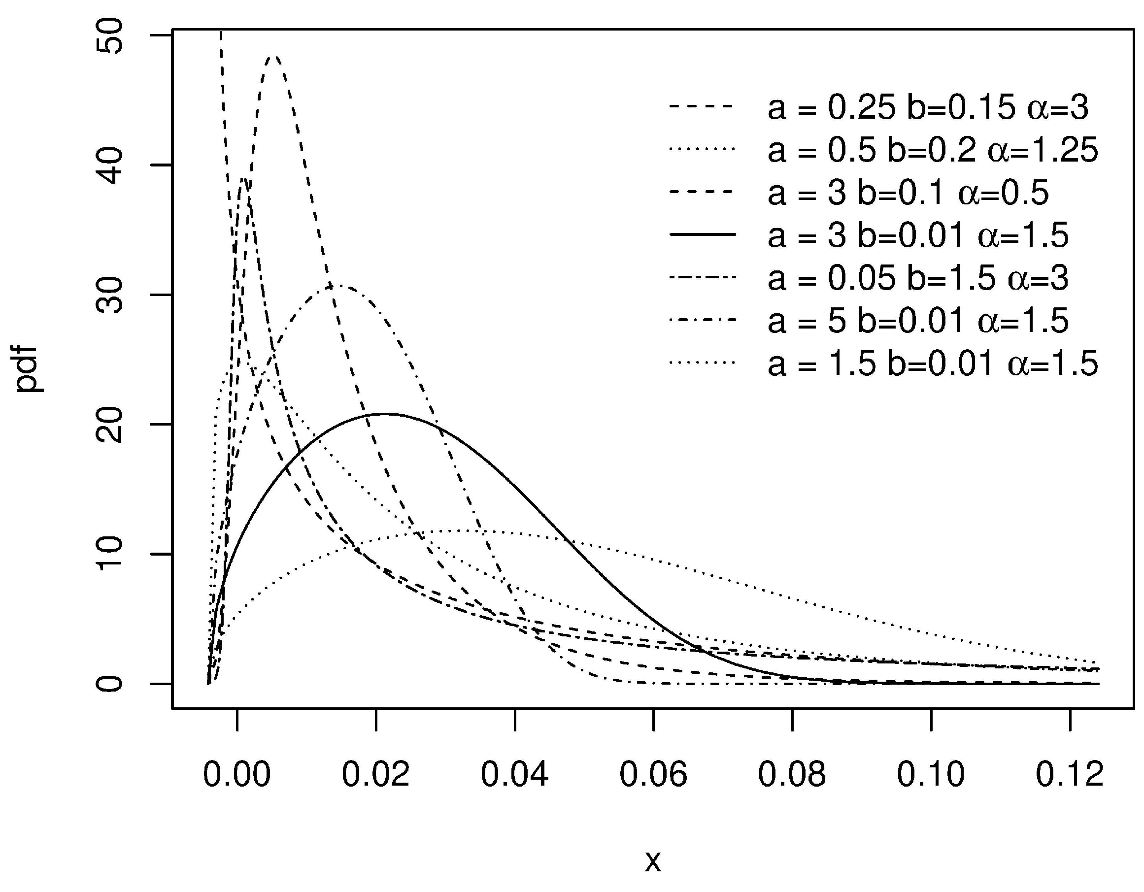
respectively, where a and $\alpha$ are shape parameters, and b and $\beta$ are scale parameters. We have $F_{NHLx}(x;\zeta )=f_{NHLx}(x;\zeta )=0$ for $x<-\beta$. Thus, the cdf has been derived from the following formula: $F_{EXL}(x;\xi )=F_{NH}\left(\frac{1}{1-F_{Lx}^{\ast }(x;\eta )};\tau \right)$, $x\in \mathbb{R}$. By taking $a=1$, we remark that $F_{NHLx}(x;\zeta )=F_{EXL}(x;\xi )$; the NHLx distribution is reduced to the EXL distribution with $\lambda =b$. The asymptotic properties of the pdf depend on the values of $\alpha$ mainly; with the use of standard asymptotic techniques, we establish that

$$\underset{x\to -\beta }{lim}{f}_{NHLx}(x;\zeta )=\left\{\begin{array}{cc}\infty \hfill & \mathrm{if}\alpha <1\hfill \\ \frac{ba}{\beta }\hfill & \mathrm{if}\alpha =1\hfill \\ 0\hfill & \mathrm{if}\alpha >1\hfill \end{array}\right.,\underset{x\to \infty }{lim}{f}_{NHLx}(x;\zeta )=0.$$

Figure 1 completes these asymptotic results by showing some curves of the pdf for several parameter values.

In Figure 1, we see that the pdf can be inverted J decreasing or have uni-modal shapes. It is very flexible to skewness, peakedness, and platness curves at a small value of $\beta$ (at least), and different selected parameter values of a, b, and $\alpha$. Such flexibility is not observed for the pdf of the EXL distribution, as visually shown in the figures in [14].

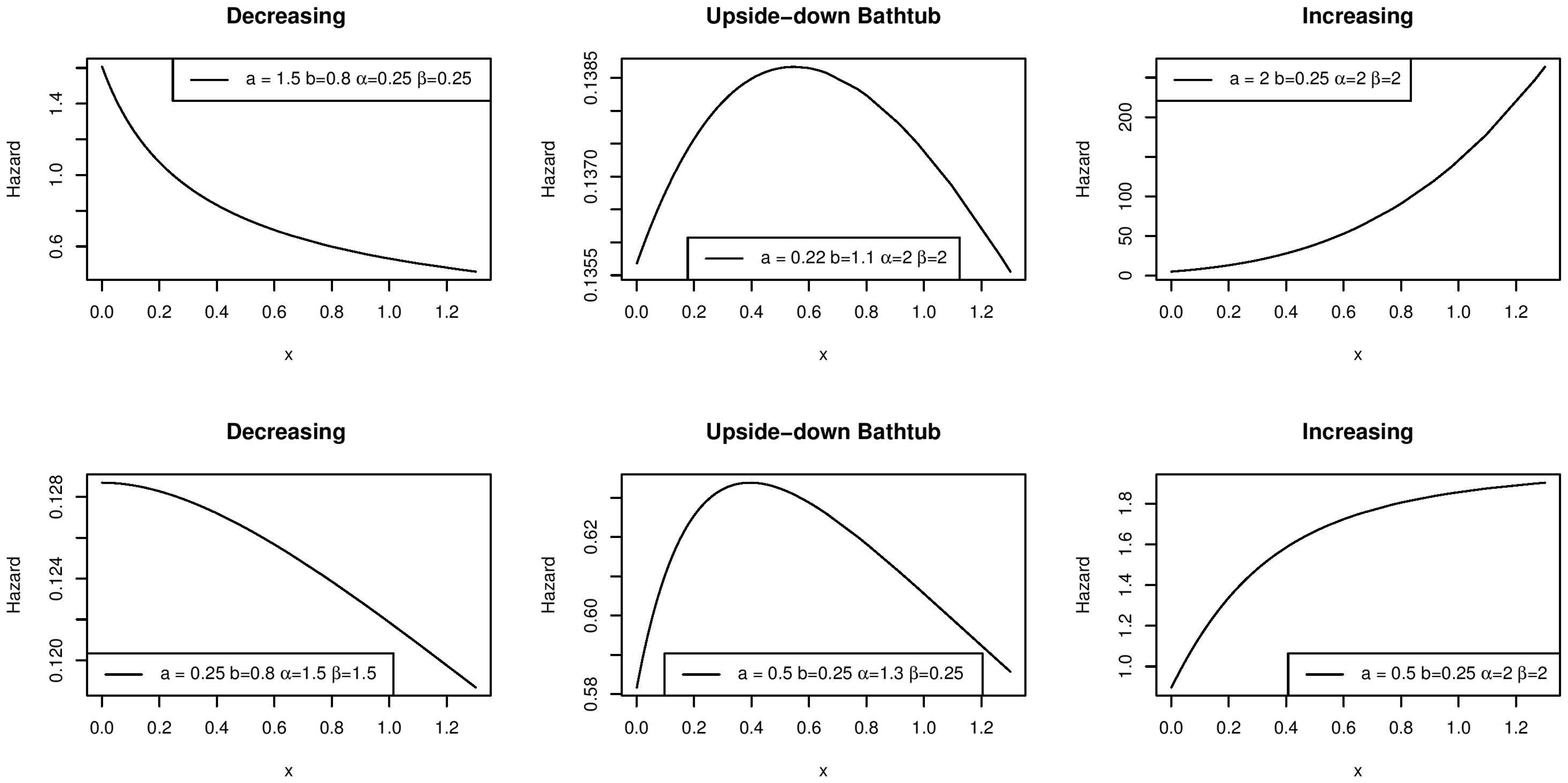
The analysis of the corresponding hrf is now examined. By applying the definition $h_{NHLx}(x;\zeta )=f_{NHLx}(x;\zeta )/[1-F_{NHLx}(x;\zeta )]$, it is given by

$$h_{NHLx}(x;\zeta )=\frac{ab\alpha }{\beta }{\left(\frac{\beta }{x+\beta }\right)}^{-\alpha +1}{\left(1+b{\left(\frac{\beta }{x+\beta }\right)}^{-\alpha }\right)}^{a-1},x\ge -\beta ,$$

and $h_{NHLx}(x;\zeta )=0$ for $x<-\beta$. Contrary to the pdf, the asymptotic properties of the hrf mainly depend on the values of a and $\alpha$; we have

$$\underset{x\to -\beta }{lim}{h}_{NHLx}(x;\zeta )=\left\{\begin{array}{cc}\infty \hfill & \mathrm{if}\alpha <1\hfill \\ \frac{ba}{\beta }\hfill & \mathrm{if}\alpha =1\hfill \\ 0\hfill & \mathrm{if}\alpha >1\hfill \end{array}\right.,\underset{x\to \infty }{lim}{h}_{NHLx}(x;\zeta )=\left\{\begin{array}{cc}\infty \hfill & \mathrm{if}a\alpha >1\hfill \\ \frac{b^a}{\beta }\hfill & \mathrm{if}a\alpha =1\hfill \\ 0\hfill & \mathrm{if}a\alpha <1\hfill \end{array}\right..$$

In full generality, the possible shapes of the hrf are determinant for modeling purposes: the more different shapes it has, the more the associated model is applicable to a wide panel of data sets.

Figure 2 presents the identified shapes for the hrf of the NHLx distribution. From Figure 2, we see that the hrf can be increasing, decreasing, or upside-down bathtub-shaped, with flexible convex–concave properties. In particular, these curve modulations are possible thanks to the variation of the new additional parameters a. We are far beyond the curve possibilities of the hrf of the EXL distribution, which is only increasing according to [14]. Thus, from one perspective, the NHLx distribution adds a new shape parameter a to the EXL distribution in a thorough fashion, considerably improving its modeling properties.

The qf of the NHLx distribution is now studied. To begin, it is defined in function of $F_{NHLx}(u;\zeta )$ by $Q_{NHLx}(u;\zeta )=F_{NHLx}^{-1}(u;\zeta )$, $u\in (0,1)$. After some mathematical development, we establish that

$$\begin{array}{c}\hfill Q_{NHLx}(u;\zeta )=\beta \left\{{\left[\frac{1}{b}\left({\left(1-log(1-u)\right)}^{\frac{1}{a}}-1\right)\right]}^{\frac{1}{\alpha }}-1\right\},u\in (0,1).\end{array}$$

Based on this qf, the main quartiles of the NHLx distribution can be explicated: by taking $u=1/4$, $u=1/2$, and $u=3/4$ into $Q_{NHLx}(u;\zeta )$, we get the first, second, and third quartiles. In addition, several quantile-based functions, and skewness and kurtosis measures, can be listed and analyzed (see [27]). In addition, various quantile regression models can be constructed (see [28]).

3. Moment Properties of the NHLx Distribution

The moment properties of the NHLx distribution are now under investigation. First, for a random variable X with the NHLx distribution and any integer r, the rth moment of X is defined by

$${\mu }_r^{\ast }=E(X^r)={\int }_{-\infty }^{\infty }{x}^r{f}_{NHLx}(x;\zeta )dx,$$

which can be explicated as

$${\mu }_r^{\ast }={\int }_{-\beta }^{\infty }{x}^r\frac{ab\alpha }{\beta }{\left(\frac{\beta }{x+\beta }\right)}^{-\alpha +1}{\left(1+b{\left(\frac{\beta }{x+\beta }\right)}^{-\alpha }\right)}^{a-1}{e}^{1-{\left(1+b{\left(\frac{\beta }{x+\beta }\right)}^{-\alpha }\right)}^a}dx.$$

For given distribution parameters, this integral can be computed numerically with the help of scientific software. An analytical expression involving sums is given in the next proposition.

Proposition 1. 

Let X be a random variable with the NHLx distribution. Then, its rth moment can be expressed as

$${\mu }_r^{\ast }={\beta }^{r}e\sum _{j=0}^r\sum _{k=0}^{\infty }\left(\genfrac{}{}{0pt}{}{r}{j}\right)\left(\genfrac{}{}{0pt}{}{\frac{j}{\alpha }}{k}\right)\frac{{(-1)}^{r-j+k}}{b^{\frac{j}{\alpha }}}\mathsf{\Gamma }\left(\frac{1}{a}\left(\frac{j}{\alpha }-k\right)+1,1\right),$$

where $e=exp(1)$ and $\mathsf{\Gamma }(x,y)={\int }_x^{\infty }{t}^{y-1}{e}^{-t}dt$ with $y\in \mathbb{R}$ and $x>0$, which defines the incomplete gamma function.

Proof. 

Let us apply the following change of variable:

$$u={\left(1+b{\left(\frac{\beta }{x+\beta }\right)}^{-\alpha }\right)}^a,du=\frac{ab\alpha }{\beta }{\left(\frac{\beta }{x+\beta }\right)}^{-\alpha +1}{\left(1+b{\left(\frac{\beta }{x+\beta }\right)}^{-\alpha }\right)}^{a-1}dx,$$

which satisfies ${lim}_{x\to -\beta }u=1$ and ${lim}_{x\to \infty }u=\infty$. Then, we have

$$\begin{array}{c}\hfill {\mu }_r^{\ast }={\beta }^{r}e{\int }_1^{\infty }{\left\{{\left[\frac{1}{b}\left(u^{\frac{1}{a}}-1\right)\right]}^{\frac{1}{\alpha }}-1\right\}}^r{e}^{-u}du.\end{array}$$

By applying the standard and generalized binomial formulas, we get

$$\begin{array}{cc}\hfill {\mu }_r^{\ast }& ={\beta }^{r}e\sum _{j=0}^r\left(\genfrac{}{}{0pt}{}{r}{j}\right)\frac{{(-1)}^{r-j}}{b^{\frac{j}{\alpha }}}{\int }_1^{\infty }{\left(u^{\frac{1}{a}}-1\right)}^{\frac{j}{\alpha }}{e}^{-u}du\hfill \\ \hfill & ={\beta }^{r}e\sum _{j=0}^r\left(\genfrac{}{}{0pt}{}{r}{j}\right)\frac{{(-1)}^{r-j}}{b^{\frac{j}{\alpha }}}\sum _{k=0}^{\infty }\left(\genfrac{}{}{0pt}{}{\frac{j}{\alpha }}{k}\right){(-1)}^k{\int }_1^{\infty }{u}^{\frac{1}{a}\left(\frac{j}{\alpha }-k\right)}{e}^{-u}du\hfill \\ \hfill & ={\beta }^{r}e\sum _{j=0}^r\sum _{k=0}^{\infty }\left(\genfrac{}{}{0pt}{}{r}{j}\right)\left(\genfrac{}{}{0pt}{}{\frac{j}{\alpha }}{k}\right)\frac{{(-1)}^{r-j+k}}{b^{\frac{j}{\alpha }}}\mathsf{\Gamma }\left(\frac{1}{a}\left(\frac{j}{\alpha }-k\right)+1,1\right).\hfill \end{array}$$

This ends the proof of Proposition 1. □

Based on Proposition 1, the mean of X can be expanded as

$${\mu }_1^{\ast }=\beta e\sum _{j=0}^1\sum _{k=0}^{\infty }\left(\genfrac{}{}{0pt}{}{1}{j}\right)\left(\genfrac{}{}{0pt}{}{\frac{j}{\alpha }}{k}\right)\frac{{(-1)}^{1-j+k}}{b^{\frac{j}{\alpha }}}\mathsf{\Gamma }\left(\frac{1}{a}\left(\frac{j}{\alpha }-k\right)+1,1\right)$$

and the moment of order 2 of X can be expressed as

$${\mu }_2^{\ast }={\beta }^{2}e\sum _{j=0}^2\sum _{k=0}^{\infty }\left(\genfrac{}{}{0pt}{}{2}{j}\right)\left(\genfrac{}{}{0pt}{}{\frac{j}{\alpha }}{k}\right)\frac{{(-1)}^{k-j}}{b^{\frac{j}{\alpha }}}\mathsf{\Gamma }\left(\frac{1}{a}\left(\frac{j}{\alpha }-k\right)+1,1\right).$$

From the above moments, we derive the variance of X by $V={\mu }_2^{\ast }-{({\mu }_1^{\ast })}^2$. Several other moment measures can be expressed in a similar manner, including the dispersion index, coefficient of variation, moment skewness, and moment kurtosis. More details on the moment skewness and moment kurtosis will be provided later.

The two following points can be proven by following the lines of the proof of Proposition 1.

• The rth moment of X about the mean can be expressed as

  $$\begin{array}{cc}\hfill & {\mu }_r=E\left[{(X-{\mu }_1^{\ast })}^r\right]\hfill \\ \hfill & ={\beta }^{r}e\sum _{j=0}^r\sum _{k=0}^{\infty }\left(\genfrac{}{}{0pt}{}{r}{j}\right)\left(\genfrac{}{}{0pt}{}{\frac{j}{\alpha }}{k}\right)\frac{{(-1)}^{r-j+k}}{b^{\frac{j}{\alpha }}}{\left(1+\frac{{\mu }_1^{\ast }}{\beta }\right)}^{r-j}\mathsf{\Gamma }\left(\frac{1}{a}\left(\frac{j}{\alpha }-k\right)+1,1\right).\hfill \end{array}$$
  Based on it, the standard moment skewness measure is defined by $SK={\mu }_3/V^{\frac{3}{2}}$, and the standard moment kurtosis measure is defined by $KU={\mu }_4/V^2$, among other moment measures.
• The rth unconditional moment of X at a certain $t>0$ can be expanded as

  $$\begin{array}{cc}\hfill & {\mu }_r(t)=E[X^r\mid X\le t]=\frac{{\beta }^{r}e}{1-e^{1-{\left(1+b{\left(\frac{\beta }{t+\beta }\right)}^{-\alpha }\right)}^a}}\sum _{j=0}^r\sum _{k=0}^{\infty }\left(\genfrac{}{}{0pt}{}{r}{j}\right)\left(\genfrac{}{}{0pt}{}{\frac{j}{\alpha }}{k}\right)\frac{{(-1)}^{r-j+k}}{b^{\frac{j}{\alpha }}}\times \hfill \\ \hfill & \left[\mathsf{\Gamma }\left(\frac{1}{a}\left(\frac{j}{\alpha }-k\right)+1,1\right)-\mathsf{\Gamma }\left(\frac{1}{a}\left(\frac{j}{\alpha }-k\right)+1,{\left(1+b{\left(\frac{\beta }{t+\beta }\right)}^{-\alpha }\right)}^a\right)\right].\hfill \end{array}$$
  It is immediate that ${lim}_{t\to \infty }{\mu }_r(t)={\mu }_r$. The unconditional moments are useful in the expression of various important functions, such as the mean residual life and reversed mean residual life functions. For more information on these functions, see [29].

4. Maximum Likelihood Estimates of the Parameters

We now consder the NHLx distribution as a statistical model, and we assume that the parameters a, b, $\alpha$, and $\beta$ are unknown. We aim to give some details on the maximum likelihood estimates (MLEs) of the parameters. First, let n be a positive integer, $X_1,X_2,\dots X_n$ be independent and identically distributed random variables drawn from the NHLx distribution, and $x_1,x_2,\dots ,x_n$ be corresponding observations. Then, provided that $inf(x_1,x_2,\dots ,x_n)\ge -\beta$, the likelihood function and log-likelihood functions are defined by

$$\begin{array}{cc}\hfill & L(x_1,x_2,\dots ,x_n;\zeta )=\prod _{i=1}^n{f}_{NHLx}(x_i;\zeta )\hfill \\ \hfill & ={\left(\frac{ab\alpha }{\beta }\right)}^n\prod _{i=1}^n{\left(\frac{\beta }{x_i+\beta }\right)}^{-\alpha +1}\prod _{i=1}^n{\left(1+b{\left(\frac{\beta }{x_i+\beta }\right)}^{-\alpha }\right)}^{a-1}{e}^{n-{\sum }_{i=1}^n{\left(1+b{\left(\frac{\beta }{x_i+\beta }\right)}^{-\alpha }\right)}^a}\hfill \end{array}$$

and

$$\begin{array}{cc}\hfill & \ell (x_1,x_2,\dots ,x_n;\zeta )=logL(x_1,x_2,\dots ,x_n;\zeta )\hfill \\ \hfill & =nlog\left(\frac{ab\alpha }{\beta }\right)+(1-\alpha )\sum _{i=1}^{n}log\left(\frac{\beta }{x_i+\beta }\right)+(a-1)\sum _{i=1}^{n}log\left(1+b{\left(\frac{\beta }{x_i+\beta }\right)}^{-\alpha }\right)\hfill \\ \hfill & +n-\sum _{i=1}^n{\left(1+b{\left(\frac{\beta }{x_i+\beta }\right)}^{-\alpha }\right)}^a,\hfill \end{array}$$

respectively. Then, the MLEs of the parameters a, b, $\alpha$, and $\beta$, say $\widehat{a}$, $\widehat{b}$, $\widehat{\alpha }$, and $\widehat{\beta }$, respectively, are defined by

$$\widehat{\zeta }=(\widehat{a},\widehat{b},\widehat{\alpha },\widehat{\beta })={argmax}_{\zeta }\ell (x_1,x_2,\dots ,x_n;\zeta ).$$

In the case where $\beta$ is known and we have surely $inf(x_1,x_2,\dots ,x_n)\ge -\beta$, the MLEs of a, b, and $\alpha$ are the solution of the following equations: $\frac{\partial }{\partial a}\ell (x_1,x_2,\dots ,x_n;\zeta )=0$, $\frac{\partial }{\partial b}\ell (x_1,x_2,\dots ,x_n;\zeta )=0$ and $\frac{\partial }{\partial \alpha }\ell (x_1,x_2,\dots ,x_n;\zeta )=0$, where

$$\begin{array}{cc}\hfill & \frac{\partial }{\partial a}\ell (x_1,x_2,\dots ,x_n;\zeta )=\frac{n}{a}+\sum _{i=1}^{n}log\left(1+b{\left(\frac{\beta }{x_i+\beta }\right)}^{-\alpha }\right)\hfill \\ \hfill & -\sum _{i=1}^n{\left(1+b{\left(\frac{\beta }{x_i+\beta }\right)}^{-\alpha }\right)}^{a}log\left(1+b{\left(\frac{\beta }{x_i+\beta }\right)}^{-\alpha }\right),\hfill \end{array}$$

$$\begin{array}{cc}\hfill & \frac{\partial }{\partial b}\ell (x_1,x_2,\dots ,x_n;\zeta )=\frac{n}{b}+(a-1)\sum _{i=0}^n{\left(1+b{\left(\frac{\beta }{x_i+\beta }\right)}^{-\alpha }\right)}^{-1}{\left(\frac{\beta }{x_i+\beta }\right)}^{-\alpha }\hfill \\ \hfill & -a\sum _{i=1}^n{\left(1+b{\left(\frac{\beta }{x_i+\beta }\right)}^{-\alpha }\right)}^{a-1}{\left(\frac{\beta }{x_i+\beta }\right)}^{-\alpha }\hfill \end{array}$$

and

$$\begin{array}{cc}\hfill & \frac{\partial }{\partial \alpha }\ell (x_1,x_2,\dots ,x_n;\zeta )=\frac{n}{\alpha }-\sum _{i=1}^{n}log\left(\frac{\beta }{x_i+\beta }\right)\hfill \\ \hfill & +(1-a)b\sum _{i=1}^n{\left(1+b{\left(\frac{\beta }{x_i+\beta }\right)}^{-\alpha }\right)}^{-1}{\left(\frac{\beta }{x_i+\beta }\right)}^{-\alpha }log\left(\frac{\beta }{x_i+\beta }\right)\hfill \\ \hfill & +ab\sum _{i=1}^n{\left(1+b{\left(\frac{\beta }{x_i+\beta }\right)}^{-\alpha }\right)}^{a-1}{\left(\frac{\beta }{x_i+\beta }\right)}^{-\alpha }log\left(\frac{\beta }{x_i+\beta }\right).\hfill \end{array}$$

The above expressions do not have closed-form solutions; hence, they are to be solved numerically by iterative methods. These numerical values can be easily obtained using specific tools in statistical software such as the R software, and the MLE of $\beta$ is obtained by taking its first-order statistics, as in [14]. It is also possible to determine the values of the standard errors (SEs) of the MLEs. For more information, see [30].

Based on the MLEs, we define the estimated pdf of the NHLx distribution by $f_{NHLx}(x;\widehat{\zeta })$. Conceptually, the curve of this estimated function must be close to the shape of the histogram of the data, among other visual criteria.

5. Simulation Study

In this section, we perform 1000 Monte Carlo simulation studies for three different sets of parameters and each of the sample sizes of $n\in \{50,100,250,500,750,1000\}$. By considering the order $(a,b,\alpha ,\beta )$, these sets of parameters are Set I $=(0.5,1.5,5,0.5)$, Set II $=(0.5,1.5,4,0.75)$, and Set III $=(1.5,0.5,4,0.5)$.

Table 1. Simulation results related to the MLEs of the NHLx model parameters.

n	$\widehat{\mathit{a}}$			$\widehat{\mathit{b}}$			$\widehat{\mathit{\alpha }}$			$\widehat{\mathit{\beta }}$
	MMLE	Bias	MSE	MMLE	Bias	MSE	MMLE	Bias	MSE	MMLE	Bias	MSE
Set I
50	2.4691	1.9691	13.3180	2.9450	1.4450	54.9364	9.2113	4.2113	310.9836	0.7425	0.2425	1.2292
100	1.9081	1.4081	3.6890	2.4782	0.9782	40.3076	6.9163	1.9163	128.6739	0.5886	0.0886	0.4186
250	1.5403	1.0403	2.0234	1.8814	0.3814	7.3395	6.0152	1.0152	58.5405	0.5465	0.0465	0.1517
500	1.2723	0.7723	0.9669	1.6510	0.1510	2.3173	5.3303	0.3303	11.0218	0.5143	0.0143	0.0322
750	1.1679	0.6679	0.6544	1.5840	0.0840	0.8996	5.1302	0.1302	2.9589	0.5053	0.0053	0.0090
1000	1.1355	0.6355	0.5534	1.5507	0.0507	0.6974	5.1039	0.1039	2.2337	0.5046	0.0046	0.0067
Set II
50	2.4179	1.9179	6.9777	3.2423	1.7423	170.7508	6.0725	2.0725	268.0909	0.8891	0.1391	1.7534
100	2.0139	1.5139	4.3307	2.3196	0.8196	34.8643	4.3855	0.3855	28.9119	0.7571	0.0071	0.1972
250	1.5278	1.0278	1.8965	1.7518	0.2518	6.5711	4.1402	0.1402	6.6622	0.7548	0.0048	0.0465
500	1.2650	0.7650	0.9185	1.6067	0.1067	1.7551	4.0561	0.0561	2.5538	0.7509	0.0009	0.0198
750	1.1526	0.6526	0.5826	1.5615	0.0615	1.0451	3.9887	−0.0113	1.1312	0.7459	−0.0041	0.0083
1000	1.1297	0.6297	0.5391	1.5262	0.0262	0.5502	3.9882	−0.0118	0.6922	0.7470	−0.0030	0.0054
Set III
50	2.6338	1.1338	6.5559	0.6993	0.1993	18.5802	5.2280	1.2280	246.0191	0.5697	0.0697	1.6784
100	2.0040	0.5040	2.9493	0.5758	0.0758	1.3542	4.7413	0.7413	46.4162	0.5341	0.0341	0.1676
250	1.5413	0.0413	1.1911	0.4969	$-0.0031$	0.1653	4.1298	0.1298	8.1507	0.5022	0.0022	0.0432
500	1.2694	$-0.2306$	0.4318	0.4946	$-0.0054$	0.0944	4.0379	0.0379	2.6806	0.4975	$-0.0025$	0.0139
750	1.1916	−0.3084	0.2963	0.4779	−0.0221	0.0413	3.9693	−0.0307	0.9247	0.4957	−0.0043	0.0055
1000	1.1182	−0.3818	0.2738	0.4934	−0.0066	0.0286	3.9998	−0.0002	0.6297	0.4989	−0.0011	0.0038

shows the mean MLEs (MMLEs), biases and mean squared errors (MSEs) of the studies.

From Table 1, it can be observed that as the sample size increases, the biases and MSEs of the MLEs decrease, and with the increase in the sample sizes, the MMLEs are closer to the true parameter values. These results prove the accuracy of the considered parameter strategy estimation.

6. Applications of the NHLx Model

6.1. Heavy-Tailed Data Applications

Two real data sets taken from [31], namely the theft and claim data, are considered to illustrate the proposed methodology. These data sets are known to have heavy tail features.

Table 2. Estimation of the tail probabilities of various distributions for the considered data sets.

Models (Theft Data)	$\mathbf{S}(8000)$	$\mathbf{S}(\mathrm{10,000})$	$\mathbf{S}(\mathrm{20,000})$
NHLx	0.12090	0.10840	0.07531
lognormal	0.05972	0.04418	0.01536
Weibull	0.03970	0.02270	0.00200
gamma	0.03755	0.01897	0.00070
exponential	1.9067 × ${10}^{-2}$	7.0851 × ${10}^{-3}$	5.0197 × ${10}^{-5}$
(Claim data)	$\mathbf{S}(\mathbf{330})$	$\mathbf{S}(\mathbf{430})$	$\mathbf{S}(\mathbf{530})$
NHLx	0.94477	0.86505	0.73682
Weibull	0.370878	0.19394	0.08713
gamma	0.34625	0.19193	0.10045
lognormal	0.32961	0.20544	0.13060
exponential	0.32557	0.23171	0.16491

presents the estimation of the tails of several standard distributions, namely the lognormal, Weibull, gamma, and exponential distributions, and the proposed NHLx distribution, taken at several values. The survival function, denoted by $S(x)$ for all distributions in full generality, determines the tail probabilities at the point x.

It is obvious from Table 2 that the NHLx model has a better fit in both data sets, and its corresponding tail probabilities are also fairly high. This means that the proposed distribution is also a heavy-tailed distribution, which was compared to other heavy-tailed distributions and contains more mass at the tail ends than the other distributions considered for comparison.

The rest of the study is devoted to the in-depth analysis of two famous data sets in the literature, highlighting the efficiency of the estimated NHLx model under real-life scenarios.

6.2. Practical Applications

The first data set contains 65 successive eruptions of the waiting times (in seconds) of the Kiama Blowhole data. It was studied in [32,33]. The second data set is about intensive care unit (ICU) patients for varying time periods of 37 patients. It was analyzed in [34] and, more recently, in [35].

The descriptive measures such as mean, median, skewness, and kurtosis have been computed for both the eruption data and ICU data sets. The results are presented in

Table 3. Descriptive measures for the two data sets.

Data Sets	Mean	Median	Skewness	Kurtosis
Eruption data	46.5486	29.3811	47.9415	43.2141
ICU data	19.9494	12.5919	47.9426	43.2148

.

From the measures of skewness and kurtosis, it is clear that the data are highly skewed and heavy-tailed. Furthermore, the mean value is larger than the median.

For comparison purposes, we consider some of the most accurate extended Lx models: the WL, EXL, and Lx models.

The MLEs and the corresponding SEs of these models are listed in

Table 4. MLEs with SEs in parentheses of the considered models for the two data sets.

Data Sets	Models	a	b	$\mathit{\alpha }$	$\mathit{\beta }$
Eruption data	NHLx	0.1052	0.0095	6.0546	7
		(0.0246)	(0.0080)	(1.2023)	(-)
	WL	1.9842	2.9883	0.1915	2.0231
		(3.8721)	(2.8437)	(0.1422)	(8.2844)
	EXL	-	1.5369	0.0452	7
			(0.1418)	(0.0016)	(-)
	Lx	-	-	1.8007	46.7964
				(0.4426)	(13.9539)
ICU data	NHLx	0.0886	0.0132	8.0704	3
		(0.0443)	(0.0381)	(4.2954)	(-)
	WL	4.3066	1.6119	0.2584	3.7699
		(5.4222)	(0.4737)	(0.1369)	(4.7682)
	EXL	-	1.4432	0.0951	3
			(0.1743)	(0.0366)	(-)
	Lx	-	-	2.7744	21.0499
				(1.2094)	(10.8889)

.

The measures of goodness of fit are used to verify whether a data set is distributionally compatible with a given model. To judge the accuracy of a model, we use the Cramér–von Mises (W*), Anderson–Darling (A*), and Kolmogorov–Smirnov (K-S) statistics (D), along with the K-S p-Value related to D. Adequacy measures are widely used to determine which model is best. Here, we traditionally consider the Akaike information criterion (AIC), consistent AIC (CAIC), Bayesian information criterion (BIC), and Hannan–Quinn information criterion (HQIC), which are based on the MLEs of the models. The model with the minimum W*, A*, D, AIC, CAIC, BIC, and HQIC value and maximum p-Value is chosen as the best one that fits the data. We may refer to [36] for the precise definitions of these measures. Their values for the considered models and the two data sets are collected in

Table 5. Values of the statistical measures for the considered models.

Models	W*	A*	D	p-Value	AIC	CAIC	BIC	HQIC
Eruption data
NHLx	0.0998	0.7471	0.0761	0.8520	592.9289	593.3289	599.4056	595.4804
WL	0.1119	0.8036	0.1062	0.4656	597.1462	597.8242	605.7818	600.5482
EXL	0.2213	1.4388	0.1230	0.2873	607.4000	607.5968	611.7178	609.101
Lx	0.1182	0.8570	0.2317	0.0021	619.4907	619.6874	623.8085	621.1917
ICU data
NHLx	0.2666	1.7021	0.2047	0.0905	242.5222	243.2495	247.355	244.226
WL	0.3459	2.1002	0.2071	0.0838	252.6803	253.9303	259.124	254.952
EXL	0.547	3.044	0.2266	0.0448	264.4479	264.8008	267.6697	265.5837
Lx	0.3404	2.0824	0.3091	0.0017	256.5615	256.9144	259.7833	257.6973

.

From Table 5, it is witnessed that the two data sets have a better fit for the proposed NHLx model than the other three models.

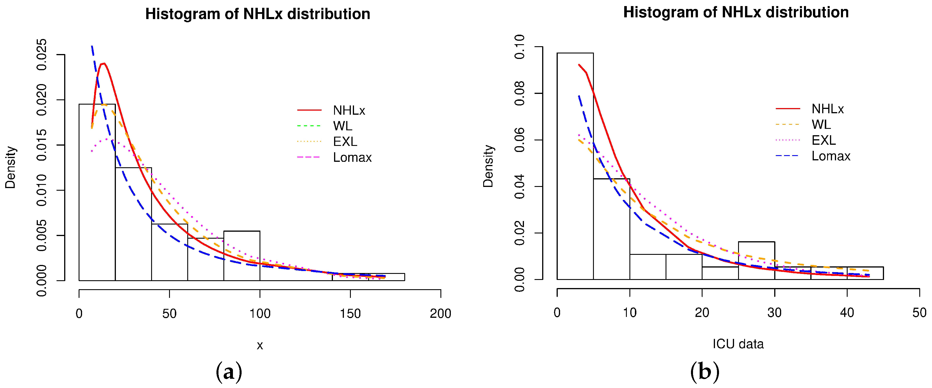
The histogram plots and estimated pdfs of the considered models are reported in Figure 3.

From Figure 3, we see that both histograms exhibit the skewed nature of the two data sets, and the estimated pdf curves depict that the NHLx model is observed to have a better pattern of closeness to the histogram plot when compared to the other three models.

7. Conclusions

In this paper, we propose a new four-parameter Lomax distribution called the Nadarajah–Haghighi Lomax distribution. It aims to provide a new lower-bounded distribution that combines the functionalities of the Nadarajah–Haghighi and Lomax distributions, and extends the modeling scope of the so-called exponential Lomax distribution. We have derived various properties, including the expression of the probability density, hazard and quantile functions, and diverse kinds of moments. The maximum likelihood method is used for estimating the model parameters. Simulation studies show its effectiveness by considering different sets of parameters. Furthermore, the support of two real data sets is taken to illustrate the applications of the Nadarajah–Haghighi Lomax distribution and it is compared with other Lomax-based distributions. From the obtained results, it is very easy to understand that the Nadarajah–Haghighi Lomax distribution has a better fit than the other Lomax models. The perspectives of new work based on the Nadarajah–Haghighi Lomax distribution are numerous, including:

• the development of various extensions, such as parametric-functional, multivariate, and discrete versions;
• the creation of new families of distributions;
• the construction of diverse regression models;
• by viewing the related cdf as a sigmoidal function, one can think of studying the “confidential intervals” (or “confidential bounds”) and “supersaturation” to the horizontal asymptote (at the median level) in the Hausdorff sense (see [37]). These two characteristics are important for researchers in choosing an appropriate model for approximating specific data from very different branches of scientific knowledge, such as computer virus propagation (see [38]).

References

- Pareto, V. Cours d’Économie Politique; Rouge: Lausanne, Switzerland, 1897; Volume II. [Google Scholar]
- Lomax, K. Business failures: Another example of the analysis of failure data. J. Am. Stat. Assoc. 1954, 49, 847–852. [Google Scholar] [CrossRef]
- Harris, C.M. The Pareto distribution as a queue service discipline. Oper. Res. 1968, 16, 307–313. [Google Scholar] [CrossRef]
- Atkinson, A.B.; Harrison, A.J. Distribution of Personal Wealth in Britain; Cambridge University Press: Cambridge, UK, 1978. [Google Scholar]
- Bryson, M.C. Heavy-tailed distributions: Properties and tests. Technometrics 1974, 16, 61–68. [Google Scholar] [CrossRef]
- Lingappaiah, G. Bayes prediction in exponential life-testing when sample size is a random variable. IEEE Trans. Reliab. 1986, 35, 106–110. [Google Scholar] [CrossRef]
- Ahsanullah, M. Record values of the Lomax distribution. Stat. Neerl. 1991, 45, 21–29. [Google Scholar] [CrossRef]
- Balakrishnan, N.; Ahsanullah, M. Relations for single and product moments of record values from Lomax distribution. Sankhya Indian J. Stat. Ser. B 1994, 56, 140–146. [Google Scholar]
- Marshall, A.W.; Olkin, I. A new method for adding a parameter to a family of distributions with application to the exponential and Weibull families. Biometrika 1997, 84, 641–652. [Google Scholar] [CrossRef]
- Chahkandi, M.; Ganjali, M. On some lifetime distributions with decreasing failure rate. Comput. Stat. Data Anal. 2009, 53, 4433–4440. [Google Scholar] [CrossRef]
- Abdul-Moniem, I.B. Recurrence relations for moments of lower generalized order statistics from Exponentiated Lomax Distribution and its characterization. J. Math. Comput. Sci. 2012, 2, 999–1011. [Google Scholar]
- Rajab, M.; Aleem, M.; Nawaz, T.; Daniyal, M. On Five Parameter Beta Lomax Distribution. J. Stat. 2013, 20, 102–118. [Google Scholar]
- Al-Jarallah, R.A.; Ghitany, M.E.; Gupta, R.C. A proportional hazard Marshall–Olkin extended family of distributions and its application to Gompertz distribution. Commun. Stat. Theory Methods 2014, 43, 4428–4443. [Google Scholar] [CrossRef]
- El-Bassiouny, A.H.; Abdo, N.F.; Shahen, H.S. Exponential Lomax Distribution. Int. J. Comput. Appl. 2015, 121, 24–29. [Google Scholar]
- Cordeiro, G.M.; Ortega, E.M.; Popovic, B.V. The Gamma–Lomax Distribution. J. Stat. Comput. Simul. 2015, 85, 305–319. [Google Scholar] [CrossRef]
- Tahir, M.H.; Cordeiro, G.M.; Mansoor, M.; Zubair, M. The Weibull–Lomax distribution: Properties and applications. Hacet. J. Math. Stat. 2015, 44, 455–474. [Google Scholar] [CrossRef]
- Mead, M.E. On five-parameter Lomax distribution: Properties and applications. Pak. J. Stat. Oper. Res. 2016, 12, 185–200. [Google Scholar]
- Rady, E.H.A.; Hassanein, W.A.; Elhaddad, T.A. The power Lomax distribution with an application to bladder cancer data. SpringerPlus 2016, 5, 1–22. [Google Scholar] [CrossRef] [Green Version]
- Hassan, A.S.; Abd-Allah, M. Exponentiated Weibull–Lomax distribution: Properties and estimation. J. Data Sci. 2018, 16, 277–298. [Google Scholar] [CrossRef]
- Nagarjuna, B.V.; Vishnu Vardhan, R. Marshall–Olkin exponential Lomax distribution: Properties and its application. Stoch. Model. Appl. 2020, 24, 161–177. [Google Scholar]
- Al-Marzouki, S.; Jamal, F.; Chesneau, C.; Elgarhy, M. Type II Topp–Leone power Lomax distribution with applications. Mathematics 2020, 8, 4. [Google Scholar] [CrossRef] [Green Version]
- Mathew, J.; Chesneau, C. Some new contributions on the Marshall–Olkin length biased Lomax distribution: Theory, modelling and data analysis. Math. Comput. Appl. 2020, 25, 79. [Google Scholar] [CrossRef]
- Nagarjuna, B.V.; Vishnu Vardhan, R.; Chesneau, C. Kumaraswamy Generalized Power Lomax Distribution and Its Applications. Stats 2021, 4, 28–45. [Google Scholar] [CrossRef]
- Nagarjuna, B.V.; Vishnu Vardhan, R.; Chesneau, C. On the Accuracy of the Sine Power Lomax Model for Data Fitting. Modelling 2021, 2, 78–104. [Google Scholar] [CrossRef]
- Murthy, D.N.P.; Xie, M.; Jiang, R. Weibull Models; John Wiley & Sons: New York, NY, USA, 2004. [Google Scholar]
- Nadarajah, S.; Haghighi, F. An extension of the exponential distribution. Statistics 2011, 45, 543–558. [Google Scholar] [CrossRef]
- Gilchrist, W.G. Statistical Modelling with Quantile Functions; Chapman & Hall/CRC: London, UK, 2000. [Google Scholar]
- Koenker, R. Quantile Regression; Cambridge University Press: Cambridge, UK, 2005. [Google Scholar]
- Cordeiro, G.M.; Silva, R.B.; Nascimento, A.D.C. Recent Advances in Lifetime and Reliability Models; Bentham Books: Sharjah, United Arab Emirates, 2020. [Google Scholar] [CrossRef]
- Casella, G.; Berger, R.L. Statistical Inference; Brooks/Cole Publishing Company: Pacific Grove, CA, USA, 1990. [Google Scholar]
- Boland, P.J. Statistical and Probabilistic Methods in Actuarial Science; CRC Press: Boca Raton, FL, USA, 2007. [Google Scholar]
- da Silva, R.V.; de Andrade, T.A.; Maciel, D.B.; Campos, R.P.; Cordeiro, G.M. A New Lifetime Model: The Gamma Extended Fréchet Distribution. J. Stat. Theory Appl. 2013, 12, 39–54. [Google Scholar] [CrossRef] [Green Version]
- Pinho, L.G.B.; Cordeiro, G.M.; Nobre, J.S. The Harris extended exponential distribution. Commun. Stat. Theory Methods 2015, 44, 3486–3502. [Google Scholar] [CrossRef]
- Kang, I.; Hudson, I.; Rudge, A.; Chase, J.G. Density estimation and wavelet thresholding via Bayesian methods: A wavelet probability band and related metrics approach to assess agitation and sedation in ICU patients. In Discrete Wavelet Transforms—A Compendium of New Approaches and Recent Applications; IntechOpen: London, UK, 2013. [Google Scholar]
- Khan, M.S.; King, R.; Hudson, I.L. Transmuted generalized exponential distribution: A generalization of the exponential distribution with applications to survival data. Commun. Stat. Simul. Comput. 2017, 46, 4377–4398. [Google Scholar] [CrossRef]
- Chen, G.; Balakrishnan, N. A general purpose approximate goodness-of-fit test. J. Qual. Technol. 1995, 27, 154–161. [Google Scholar] [CrossRef]
- Sendov, B. Hausdorff Approximations; Kluwer: Boston, MA, USA, 1990. [Google Scholar]
- Iliev, A.; Kyurkchiev, N.; Rahnev, A.; Terzieva, T. Some Models in the Theory of Computer Viruses Propagation; LAP LAMBERT Academic Publishing: Saarbrucken, Germany, 2019. [Google Scholar]
Figure 1.
Curves of the pdf of the NHLx distribution for various parameter values, but with the fixed value: .
Figure 2.
Curves of the hrf of the NHLx distribution for various parameter values.
Figure 3.
Curves of the estimated pdfs of the considered models for the two data sets. (a) Eruption data. (b) ICU data.