
A Time-Domain Artificial Boundary for Near-Field Wave Problem of Fluid Saturated Porous Media


1
School of Civil Engineering, North China University of Technology, Beijing 100144, China
2
Key Laboratory of Urban Security and Disaster Engineering, Ministry of Education, Beijing University of Technology, Beijing 100124, China
*
Author to whom correspondence should be addressed.
Math. Comput. Appl. 2022, 27(4), 71; https://doi.org/10.3390/mca27040071
Submission received: 10 July 2022
/
Revised: 15 August 2022
/
Accepted: 16 August 2022
/
Published: 18 August 2022
Abstract
:The near-field wave problem of the saturated soil involves the energy radiation effect of the truncated infinite media. A viscous spring boundary is proposed for the fluid-saturated porous media. Based on the process of wave propagation under internal point source, the stress and flow velocity boundaries are constructed by reasonable assumptions of outgoing waves and Green’s function, respectively. Without the permeability assumption, the proposed boundary avoids the low accuracy caused by the assumption of zero permeability that is widely used in the existing methods. The boundary simultaneously has a simple form, clear physical meaning, and less computational cost due to its local character. Meanwhile, a completely explicit integration algorithm considering the damping is constructed to solve the finite element equations of saturated porous media with the proposed boundary. The accuracy and high computational efficiency of the wave numerical method are verified in the examples.
1. Introduction
The wave problem of saturated two-phase porous media is an important research issue of soil dynamics and geotechnical seismic engineering. For the problem, Biot [1] established the three-dimensional quasi-static consolidation theory by considering the deformation of solid and liquid phases, as well as the fluid-solid coupling of saturated porous media. Based on this, Biot wave theory is proposed by adding the inertial terms of soil skeleton and pore fluid [2,3]. However, there are several elastic coefficients with relatively abstract meanings in the equations, and the concept of additional mass density describing the coupling of solid and fluid lacks physical meaning, which makes it relatively difficult to measure. Therefore, many scholars improved Biot theory furtherly [4,5,6,7]. The dynamic equations proposed by Zienkiewicz [7,8] is essentially equivalent to the Biot theory. In the equations, the additional mass density is ignored and assumes that dynamic permeability coefficient considers the fluid viscosity. Men et al. [9] and Chen et al. [10] considered the incompressibility and compressibility of the pore fluid, respectively, and gave the dynamic governing equations for saturated porous media under the two conditions. Wu [11] compared the dynamic equations proposed by Biot theory and Zienkiewicz, proved that the two equations are equivalent, and gave the corresponding relationships between the corresponding parameters. Zhao et al. [12] used inductive and deductive methods to review the existing wave theory of porous media. Morency and Tromp [13] presents a numerical implementation of poroelastic wave propagation using a spectral element method, based upon an averaging technique which accommodates the transition from the microscopic to the macroscopic scale. Puente and Dumbser [14] introduced a local space-time discontinuous Galerkin method with arbitrary high-order accuracy to simulate wave propagation in poroelastic material. Wang et al. [15] investigated the wave propagation in 2D periodic fluid-saturated porous media with an isotropic or a transversely isotropic matrix.
For the near-field wave problems, absorbing artificial boundary are needed to model waves propagation in infinite field, to ensure waves have no reflection effect when passing through the artificial boundary [16]. The wave transmission boundary mainly includes [17] global precise artificial boundaries [18,19,20] and local artificial boundaries [21,22,23,24,25,26,27]. The global artificial boundary mainly includes boundary element method [28], thin layer method [29], exact Kirchhoff integration method [18,19] and Dirichlet-to-Neumann method [20,30]. The boundary conditions are established based on the initial boundary value conditions of the truncated media and are gotten through rigorous analytical derivation, leading to complicated calculation process and low efficiency. Local artificial boundaries include the viscous boundaries [21,31], the viscous-spring boundaries [22,23,24,32,33,34,35], the superposition boundaries [25,36], the extrapolation boundaries [26,37], the paraxial boundaries [38,39], the multi-directional boundary [27,40], the perfectly matched layer [41,42], and the dynamic infinite element [43,44,45]. The local artificial boundary is local both in space and time domain, that is, the responses of the target node are only related to the responses of the adjacent nodes. It has less calculation amount and higher calculation efficiency.
For the fluid saturated porous media, Modaressi and Benzzenati [46,47] established paraxial boundaries for the u-p formulation and obtained the zero-order and first-order paraxial boundary conditions, where the zero-order paraxial boundary is equivalent to the viscous boundary. Akiyoshi et al. [48] established paraxial boundaries for the u-w, u-U, and u-p models of linear and isotropic saturated soils, and extended their work to the case of laterally isotropic and anisotropic saturated soils [49,50]. The above research work is based on plane waves. Liu Guanglei and Song Erxiang [51] prop osed a viscous spring artificial boundary for the u-p equation based on cylindrical waves. Du Xiuli et al. [52] and Zhao Chenggang et al. [53,54] established two viscous spring artificial boundaries based on u-U formulation. To improve the accuracy of artificial boundaries, Li Peng and Song Erxiang [55] proposed a new high-precision artificial boundary on the basis of the work of Song Erxiang [51]. Degrande and De Roeck [56,57] proposed a global artificial boundary in the frequency domain, but its computational cost is higher. Then, under the assumptions of zero and infinity permeability coefficient, Gajo et al. [58] as well as Zerfa and Loret [59] established, respectively, two viscous boundary conditions with high computational efficiency in the time domain.
The assumption of permeability coefficient leads to neglect of fluid-solid coupling, resulting in the low accuracy of dynamic responses of the fluid saturated porous media. A new viscous spring artificial boundary without the permeability coefficient assumption is proposed based on the u-p equation of the saturated porous media. Green’s function is firstly used to establish the flow boundary velocity condition due to the similar principle by describing the pore pressure field generated by the point force. A completely explicit integration algorithm considering the damping is constructed to solve the finite element equations of saturated porous media with the proposed boundary. Finally, three examples are used to show the accuracy and effectiveness of the proposed method by comparing with analysis solutions and numerical solutions of existing boundary.
2. Wave Velocity
The propagation of waves in the semi infinitely field of saturated soil under point force is shown in Figure 1, which can be described by u-p equation. Ignoring the body force, the u-p formed control equations of fluid-saturated porous media are expressed as:
where λ and G are the Lamb constants of the soil. α and are the compressive coefficient of the soil skeleton and pore fluid, respectively. is the dynamic permeability coefficient. represents the density of the total solid-fluid mixture. . u and p represent the displacement and pore pressure of saturated soil, respectively.
Equations (1) and (2) are further transformed into the frequency domain, and the following equations are obtained by introducing the parameter :
where ω represents the circular frequency, and the displacement and pore pressure are expressed by the rotational and irrotational potential functions of P1, P2, and S waves as shown in Equations (5) and (6):
where and represent the potential function of P1 and P2 waves, respectively; represents the potential function of S wave; e is the unit vector. At the same time, and in Equation (6) are calculated as shown:
Substituting Equations (5) and (6) into Equations (3) and (4), the wave equations expressed by the potential functions of P1, P2, and S waves are obtained as follows:
where, , , and , shown in Equation (10), are the nominal wave velocity of P1, P2, and S waves [60], respectively.
As shown in Equation (10), all nominal wave velocities of three body waves are complex numbers, which are uniformly expressed in the following complex form:
The real part of the wave velocity in the equation represents the actual wave velocity of the wave, and the imaginary part reflects the attenuation of wave. Therefore, the real part of the wave velocity corresponding to the P1, P2, and S waves is the actual wave velocity of the three types of waves in saturated soil.
3. Viscous-Spring Artificial Boundary
In Figure 1, the surface of the semi-infinite saturated soil space is a free drainage boundary, and the artificial boundary is introduced to divide the semi-infinite space into two parts: the interior domain and the exterior domain . The interior domain may have complex geometry and material properties, and convenient for solving using the finite element method. The infinite exterior domain is approximated as a uniform media of linear elasticity, and the effect of the exterior domain on the interior domain is generally achieved through artificial boundaries. For this problem, the displacement u and pore pressure p, the total stress σ, and the fluid phase flow velocity Φ of the interior domain and exterior domain should satisfy the continuous conditions, shown as follows:
where σ represents the total stress of soil, and Φ is the flow velocity of pore fluid in saturated soil. Therefore, the flow velocity condition and stress condition should be satisfied on the artificial boundary.
3.1. Flow Velocity Boundary Condition
The wave propagation problem under the action of a point source on the surface of the interior domain is similar to the significance of Green’s function of the diffusion equation, that is, the field distribution generated by a unit point source. At the same time, the Lamb problem [61] analyzes the distribution of a variable field under the action of a concentrated force or point source on the surface of infinite space, such as pore water pressure in a saturated soil field under a point force. To obtain the pore pressure value on the artificial boundary, Green’s function constructs the pore pressure field distribution of fluid-saturated porous media under the action of interior concentrated force. Therefore, Equation (2) is converted into the equation as follows in two-dimensional plane polar coordinates without considering the exterior loading and ignoring the coupling term :
where r represents the outer normal direction of the artificial boundary, and t is time. It can be seen that Equation (14) is the standard form of the diffusion equation. In the infinite domain, based on Equation (14), the Green’s function [62] for the pore pressure p is obtained, and its distribution form is shown as follows:
By utilizing the relationship between the flow velocity and the pore pressure , the flow velocity boundary condition expressed in terms of pore pressure is shown below:
where p and Φ are the pore pressure and the flow velocity in the outward normal direction of the artificial boundary. Since the seepage process is a time-varying diffusion process of pore fluid in saturated porous media, only when the wave propagates to the artificial boundary is there a pressure gradient between the artificial boundary and the internal domain of soil. Therefore, Equation (16) can be further written as:
where lr is defined as the distance from the geometric center of the interior domain to the point on the artificial boundary; is the shortest time for the wave to propagate to the artificial boundary.
3.2. Stress Boundary Condition
Since Equations (8) and (9) are standard wave equations, to simplify the analysis, based on Equations (5)–(9), the outgoing wave of displacement can be assumed to be:
where n and ⊥ represent the outer normal and tangent direction of the artificial boundary, respectively; and the are solid phase displacement in the outer normal and tangent directions of the artificial boundary, respectively; v1 and v2 are the actual wave velocities in the normal and tangential of the artificial boundary, respectively; f represents the arbitrary waveform function; k1 and k2 represent wave numbers of attenuated and non-attenuated waves, respectively; l is the dimensional coordination factor; and represents the geometric attenuation factor.
Using the constitutive relationship and geometric relationship of the saturated two-phase porous media, the relationship between the total stress, displacement, and the pore pressure of saturated porous media is given:
where and are the normal and tangential stresses of the solid-phase media, respectively; τ is the shear stress of the solid-phase media. In two dimensions, when the outgoing wave propagates along the outer normal direction of the artificial boundary, the stress at the artificial boundary, i.e., Equation (20), can be further simplified to:
Substitute Equation (18) into Equation (21) to obtain the normal stress represented by the waveform function f:
By calculating the first derivative of Equation (18) with respect to time t, the relationship between the normal velocity and the waveform function f is obtained as follows:
Using Equations (18), (23), and (24) to eliminate the waveform function f, the relationship between the normal stress, displacement, velocity, and pore pressure is expressed as:
By introducing dimensionless parameters and , the normal stress boundary condition is further written as:
where the parameter A reflects the propagation characteristics of the outgoing wave, namely the amplitude ratio between the plane wave and the scattering wave; the parameter B represents the average wave velocity characteristics of the incident multi-sub-wave at different angles, namely, the relationship between the physical wave velocity and the apparent wave velocity. Through a large number of numerical calculations, the optimal values of A and B are obtained. A = 0.8, B = 1.1 [16].
Using a similar calculation process, the tangential stress boundary condition is shown below:
where the definitions of parameters A and B are the same as in Equation (26).
3.3. Finite Element Discretization of Artificial Boundary
The artificial boundary Equations (17), (26), and (27) are written in discrete form as follows:
where the superscript (l) represents the artificial boundary; ∞ represents the exterior domain; Bi represents the ith node on the boundary; and are the stress and the flow velocity of the ith node on the boundary, respectively; and are the displacement and the pore pressure of the ith node on the boundary, respectively. The variable matrices and scalar coefficients in Equations (28) and (29) are expressed in the following form:
where Li represents the boundary length corresponding to the boundary node i. Converting Equations (28) and (29) from the local coordinate system into the global coordinate system, we get:
In Equations (34) and (35), the physical meanings of each matrix and scalar coefficient are the same as that in Equations (28) and (29), and the coordinate transformations are carried out through the following relationships:
where is the coordinate transformation matrix for transforming local coordinates to global coordinates. is the cosine of the angle between the positive direction of the local coordinate r-axis and the positive direction of the global coordinate x-axis. The rest of the parameters are similar to the definition of lxy.
After discretization by the Galerkin finite element method, the dynamic governing equations of the saturated two-phase porous media, Equations (1) and (2), are represented by block matrices of internal domain and boundary:
where the subscripts B and I correspond to the nodes at the boundary and the internal domain, respectively; M is the mass matrix; K is the stiffness matrix; Q is the coupling matrix; S is the fluid compression matrix; J is the fluid permeability matrix. fuI and fqI represent the loading and fluid injection point source of the internal domain, respectively. fuB and fqB represent the effect of the exterior domain on the internal domain, namely the artificial boundary conditions (34) and (35), respectively.
At the same time, substituting Equations (34) and (35) into Equations (38) and (39), the finite element discrete equations of saturated porous media considering the boundary conditions are obtained:
where , , , and are calculated by Equations (36) and (37), respectively. The finite element discrete equations of saturated porous media can be calculated by different time domain integration methods. The proposed artificial boundary actually only changes the values of the corresponding boundary nodes on the diagonal of the coefficient matrices in Equations (40) and (41). The finite element discrete equations of saturated porous media considering the boundary conditions can be solved by a completely explicit integration algorithm efficiently, which is shown in Appendix A.
The proposed artificial boundary has a simple form and is easily applied to the finite element method. Since the boundary has a local approximate form both in the space and time domains, it has low computational cost and high computational efficiency. Effective calculation accuracy can be guaranteed when the artificial boundary is set at a sufficient distance from the internal source.
4. Numerical Studies
4.1. Example 1
The computational model of one-dimensional saturated soil is shown in Figure 2. Both lateral sides of the model are fixed impermeable boundaries. The top surface is a permeable boundary and is applied a uniform constant loading of 1.0 Pa. The models (a)–(c) have different bottom boundaries, such as remote boundary, fixed boundary, and artificial boundary, respectively. For the model (a), the truncated boundary is set far enough away from the load center, and within the effective calculation time, the reflected wave generated by the boundary cannot propagate to the concerned calculation area. The numerical solutions of the model (a) can be used as reference solutions for comparison. For model (b) and model (c), the truncation boundaries have the same distance from the load center and are much closer than the remote boundary. However, the truncation boundary of model (b) is a fixed boundary, while the truncated boundary of model (c) is set to the proposed artificial boundary. The material parameters of the model, taken from Simon [63] are shown in Table 1 for the values of Material 1. The analytical solutions of the one-dimensional problem of saturated soil proposed by Simon [63] are used as the reference solution and are compared with the results of the remote boundary and the fixed boundary to verify the correctness of the artificial boundary proposed in this paper.
The time-history responses of nodes 5 m and 45 m away from the load center are, respectively, selected for comparison. The time-history results of the displacement and pore pressure calculated by the three models are shown in Figure 3. It can be seen from the figure that the analytical solutions and the calculation results of the far boundary are almost completely resumed. Both results are used as the reference solutions. However, the difference between the responses of the fixed boundary and the reference solution is large, indicating that the bottom fixed boundary produces an unreal reflected wave propagating to the target node, which affects the real responses of the node. The vertical displacements and pore pressure of the model with the proposed boundary are consistent with the reference solutions, which verifies the correctness of the proposed boundary. Although the pore pressure response of the node at 5 m depth from the soil surface has some oscillations at the initial stage of the calculation, the oscillation gradually decreases as time goes on.
4.2. Example 2
The calculation model of saturated soil in two-dimensional semi-infinite space is shown in Figure 4. A semi-infinite domain model including the calculation domain with an intercepted area of 20 m × 20 m, as shown in Figure 4b. The top surface of the model is the drainage boundary and is loaded with locally uniform sine loading. The viscous spring boundaries proposed by Liu et al. [51], the remote boundary, fixed boundary, and paraxial boundary proposed by Akiyoshi et al. [48], as well as the boundary proposed in this paper, are respectively applied at the intercepted boundary. By comparing with the results of the artificial boundaries mentioned above, the accuracy and advantages of the proposed boundary are illustrated. The position of the remote boundary is selected according to the following method as an example. During the time 2.0 s of the sine loading, namely, the whole calculation time, the wave propagates at the faster velocity of P wave in the soil and is reflected by the remote boundaries. However, the reflected wave is not transmitted to the node of interest within the calculation time. The locations of the remote boundaries are set at the minimum computational domain range that does not affect the dynamic responses of the interest nodes. The material parameters in the example refer to Simon [63] and are shown in Table 1 for the values of Material No. 2.
In Figure 5, taking the numerical results of the model using the remote boundary as the reference solution, the displacement and pore pressure time histories of the fixed boundary are far from the results of the reference solution. The calculation results of the proposed boundary, the paraxial boundary, and the existing viscous spring boundaries [51] are in good agreement with the reference solutions. Moreover, the proposed boundary is more accurate than the viscous spring boundary [51], which shows the accuracy of the artificial boundary proposed in this paper.
Under the same calculation conditions and calculation method in time domain, the total computational times of the models with different boundaries mentioned above are shown in Figure 6. Among them, when the time step of the paraxial boundary is set to 5 × 10⁻⁴ s, the calculation does not converge. In the case of the remote boundary, the element number of the model is 4000, and the calculation time is 5841.81 s. Comparing several boundaries, the proposed boundary takes the shortest calculation time, which is 65.01 s. It can be seen that the proposed method has significant advantages in shortening the calculation time and improving the calculation efficiency.
4.3. Example 3
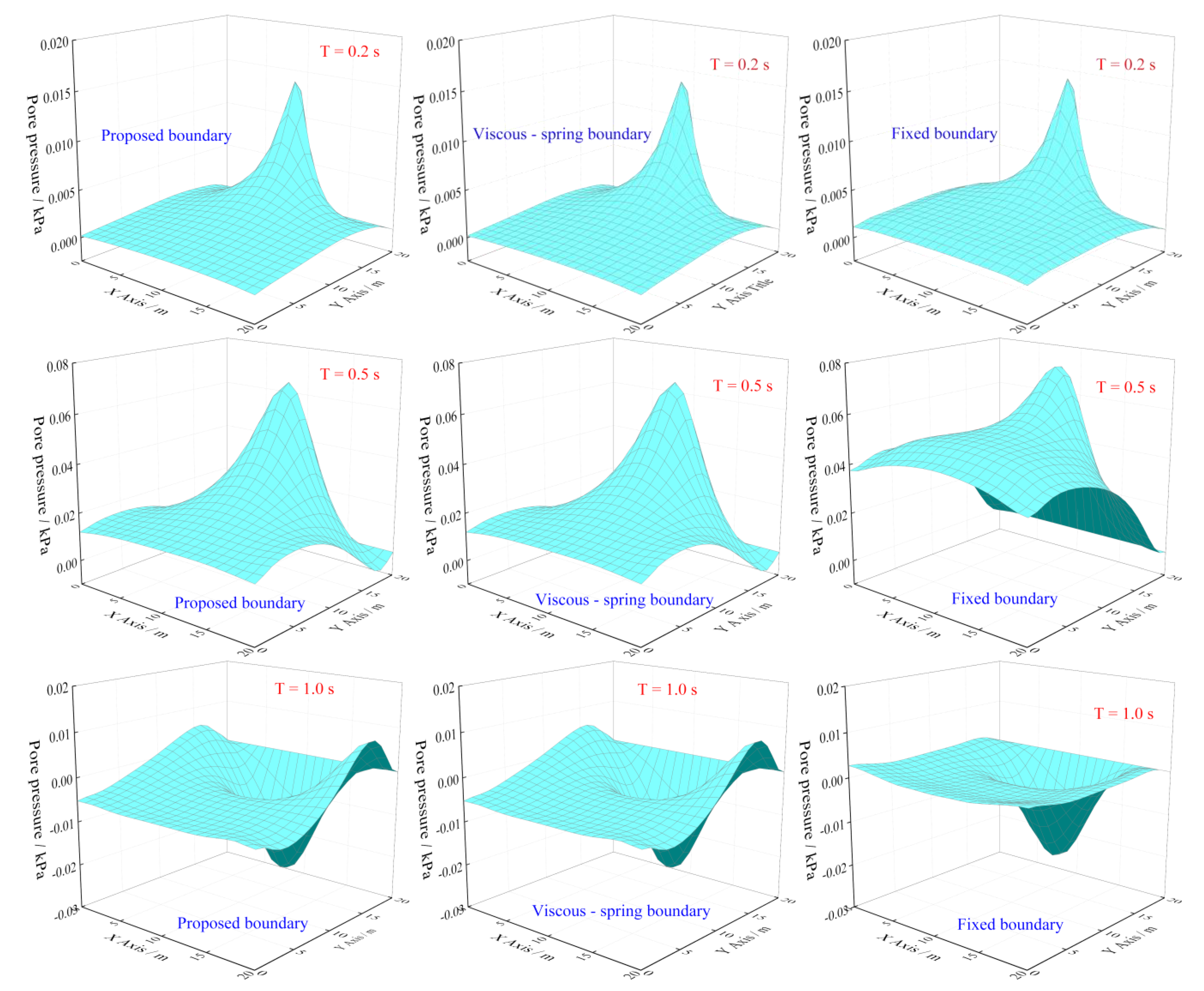
The development of displacement and pore pressure of saturated soil changed under point loading is analyzed by Example 3. A concentrated impulse loading acted on the free-draining surface of the computational model, as shown in Figure 7, and an area of 20 m × 20 m is intercepted by three different boundary conditions, namely the proposed boundary, the viscous spring boundary [51] and the fixed boundary. The changes of displacement and pore pressure in the calculation area at different time points are analyzed. Moreover, the correctness of the proposed method is further verified by comparing the three boundary conditions.
Figure 8 and Figure 9 show the distribution of displacement and pore pressure under three boundary conditions at 0.2 s, 0.5 s, and 1.0 s, respectively. From the figures, it can be seen that the influence area under the impulsive loading continues to increase with the calculation time. The formed displacement and pore pressure field continue to spread out from the point loading, and the displacement and pore pressure reach the maximum value at 0.5 s, which is the peak time of the impulsive loading. By comparing the numerical results of computational models considering the three kinds of boundary conditions, the numerical results of the proposed boundary and viscous spring boundary are the same, but the displacement and pore pressure results of the fixed boundary are completely different from that of the viscous spring boundaries. The forms of boundary conditions have a greater impact on the results of the interior domain.
5. Conclusions
For the energy radiation problem caused by the finite processing of the infinite model, a viscous spring boundary is proposed for the fluid-saturated porous media. The proposed method is illustrated the computational advantages and accuracy by theoretical method and numerical computation.
- The viscous spring boundary is composed of the stress and flow velocity boundary conditions, which are constructed by the reasonable outgoing wave assumption and Green’s function. The boundary has a simple form and clear physical meaning. Since the overall system equations considering artificial boundaries only need to change the values of the corresponding boundary nodes on the diagonal of the coefficient matrices, the boundary can be easily applied to the finite element method.
- Without the assumption of permeability and using the real wave velocity, the proposed boundary has higher accuracy than the existing boundaries with the assumption of impermeability.
- After considering the viscous spring boundary, the computational system is expressed as lumped mass equations with damping. A complete explicit integration algorithm with second-order accuracy is constructed to solve the equations.
The proposed method can be used to analyze the saturated soil-structure dynamic interaction in finite domain efficiently. The artificial boundary controls the number of degrees of freedom of the site model, and the explicit method considering the damping term also improves the calculation efficiency.
Author Contributions
Methodology, J.S.; software, J.S.; Writing—original draft, F.W.; Writing—review & editing, K.J. and H.S. All authors have read and agreed to the published version of the manuscript.
Funding
This research was funded by [National Natural Science Foundation of China] grant number [51808006], [Natural Science Foundation of Beijing] grant number [8192012], and [Yuyou Team Training Program of North China University of Technology] grant number [10751360022XN699].
Acknowledgments
The authors would like to thank the National Natural Science Foundation of China (Grant No. 51808006), the Natural Science Foundation of Beijing, China (Grant No. 8192012), and Yuyou Team Training Program of North China University of Technology (Grant No. 10751360022XN699) for funding the work presented in this paper.
Conflicts of Interest
The authors declare no conflict of interest.
Appendix A
Explicit Integration Algorithm
To simplify the analysis process, Equations (40) and (41) can be further written as follows:
where
There is a damping term in Equation (A1). Based on the explicit algorithm [64] for single-phase medium and the Euler predictor-corrector method [65], the explicit integration algorithm for two-phase media is constructed. The computational process in one time step is shown as follows:
- (a)
- The whole of the loading time is divided into several time intervals with a time step , and any time can be expressed as , (k = 1, 2, 3, …). Equation (A1) is solved using the explicit algorithm method [64] to obtain the step-by-step recurrence formula of the solid phase displacement at the time :
- (b)
- To express the acceleration at the time , convert Equation (A1) into the following form:
- (c)
- Apply the Newmark method to get the velocity at the time . The parameters ,where , , , and are known items.
- (d)
- Equation (A2) is solved using the Euler predictor-corrector method [65]. The formulas are shown as follows:
The predictor value firstly is calculated using Equation (A8), and then the predictor value and known variable , which is obtained by Equation (A7), are substituted into Equation (A9) to calculate the corrector value, that is, the pore pressure at the time .
To sum up, Equations (A5)–(A9) represent the integration algorithm of the lumped-mass equations with damping. The algorithm is a completely explicit algorithm with second-order accuracy.
References
- Biot, M.A. General theory of three-dimensional consolidation. J. Appl. Phys. 1941, 12, 155–164. [Google Scholar] [CrossRef]
- Biot, M.A. Theory of propagation of elastic waves in a fluid-saturated porous solid. I. Low-frequency range. J. Acoust. Soc. Am. 1956, 28, 168–178. [Google Scholar] [CrossRef]
- Biot, M.A. Theory of propagation of elastic waves in a fluid-saturated porous solid. II. Higher frequency range. J. Acoust. Soc. Am. 1956, 28, 179–191. [Google Scholar] [CrossRef]
- Lévy, T. Propagation of waves in a fluid-saturated porous elastic solid. Int. J. Eng. Sci. 1979, 17, 1005–1014. [Google Scholar] [CrossRef]
- Auriault, J.L. Dynamic behaviour of a porous medium saturated by a Newtonian fluid. Int. J. Eng. Sci. 1980, 18, 775–785. [Google Scholar] [CrossRef]
- Prevost, J.H. Nonlinear transient phenomena in saturated porous media. Comput. Methods Appl. Mech. Eng. 1982, 30, 3–18. [Google Scholar] [CrossRef]
- Zienkiewicz, O.C.; Shiomi, T. Dynamic behaviour of saturated porous media; the generalized Biot formulation and its numerical solution. Int. J. Numer. Anal. Methods Geomech. 1984, 8, 71–96. [Google Scholar] [CrossRef]
- Zienkiewicz, O.C.; Chan, A.H.C.; Pastor, M.; Schrefler, B.A.; Shiomi, T. Computational Geomechanics with Special Reference to Earthquake Enineering; John Wiley & Sons: New York, NY, USA, 1998. [Google Scholar]
- Men, F.L. Wave propagation in fluid-saturated porous media. Acta Geophys. 1981, 24, 65–75. (In Chinese) [Google Scholar]
- Chen, L.Z.; Wu, S.M.; Zeng, G.X. Propagation of elastic waves in saturated soil. Acta Mech. 1987, 19, 276–283. (In Chinese) [Google Scholar]
- Wu, S.M. Waves in Soil; Science Press: Beijing, China, 1997. (In Chinese) [Google Scholar]
- Zhao, C.G.; Du, X.L.; Cui, J. Advances in wave theory and numerical simulation in solid and fluid multiphase porous media. Adv. Mech. 1998, 28, 83–91. (In Chinese) [Google Scholar]
- Morency, C.; Tromp, J. Spectral-element simulations of wave propagation in porous media. Geophys. J. Int. 2008, 175, 301–345. [Google Scholar] [CrossRef]
- De la Puente, J.; Dumbser, M.; Käser, M.; Igel, H. Discontinuous Galerkin methods for wave propagation in poroelastic media. Geophysics 2008, 73, T77–T97. [Google Scholar] [CrossRef]
- Wang, Y.F.; Liang, J.W.; Chen, A.L.; Wang, Y.S.; Laude, V. Evanescent waves in two-dimensional fluid-saturated porous metamaterials with a transversely isotropic matrix. Phys. Rev. B 2020, 101, 184301. [Google Scholar] [CrossRef]
- Zhao, M. A Comparative Study of Viscoelastic Artificial Boundaries and Their Transmission Artificial Boundaries; Beijing University of Technology: Beijing, China, 2004. (In Chinese) [Google Scholar]
- Zhao, M.; Du, X.L.; Liu, J.B.; Liu, H. Explicit finite element artificial boundary scheme for transient scalar waves in two-dimensional unbounded waveguide. Int. J. Numer. Methods Eng. 2011, 87, 1074–1104. (In Chinese) [Google Scholar] [CrossRef]
- Teng, Z.H. Exact boundary condition for time-dependent wave equation based on boundary integral. J. Comput. Phys. 2003, 190, 398–418. (In Chinese) [Google Scholar] [CrossRef]
- Givoli, D.; Cohen, D. Nonreflecting Boundary Conditions Based on Kirchhoff-Type Formulae. J. Comput. Phys. 1995, 117, 102–113. [Google Scholar] [CrossRef]
- Givoli, D. Exact Representations on Artificial Interfaces and Applications in Mechanics. Appl. Mech. Rev. 1999, 52, 333–349. [Google Scholar] [CrossRef]
- Lysmer, J.; Kuhlemeyer, R.L. Finite dynamic model for infinite media. J. Eng. Mech. Div. 1969, 95, 859–878. [Google Scholar] [CrossRef]
- Deeks, A.J.; Randolph, M.F. Axisymmetric time-domain transmitting boundaries. J. Eng. Mech. 1994, 120, 25–42. [Google Scholar] [CrossRef]
- Kellezi, L. Local transmitting boundaries for transient elastic analysis. Soil Dyn. Earthq. Eng. 2000, 19, 533–547. [Google Scholar] [CrossRef]
- Liu, J.B.; Du, Y.; Du, X.L.; Wang, Z.; Wu, J. 3D viscous-spring artificial boundary in time domain. Earthq. Eng. Eng. Vib. 2006, 5, 93–102. (In Chinese) [Google Scholar] [CrossRef]
- Smith, W.D. A nonreflecting plane boundary for wave propagation problems. J. Comput. Phys. 1974, 15, 492–503. [Google Scholar] [CrossRef]
- Liao, Z.P.; Wong, H.L. A transmitting boundary for the numerical simulation of elastic wave propagation. Int. J. Soil Dyn. Earthq. Eng. 1984, 3, 174–183. (In Chinese) [Google Scholar] [CrossRef]
- Higdon, R.L. Radiation boundary conditions for elastic wave propagation. SIAM J. Numer. Anal. 1990, 27, 831–869. [Google Scholar] [CrossRef]
- Hall, W.S.; Oliveto, G. Boundary Element Methods for Soil-Structure Interaction; Springer Science and Business Media: Berlin/Heidelberg, Germany, 2003. [Google Scholar]
- Kausel, E. Thin-layer method: Formulation in the time domain. Int. J. Numer. Methods Eng. 1994, 37, 927–941. [Google Scholar] [CrossRef]
- Givoli, D. Recent advances in the DtN FE method. Arch. Comput. Methods Eng. 1999, 6, 71–116. [Google Scholar] [CrossRef]
- Kuhlemeyer, R.L.; Lysmer, J. Finite element method accuracy for wave propagation problems. J. Soil Mech. Found. Div. 1973, 99, 421–427. [Google Scholar] [CrossRef]
- Du, X.L. Locally decoupled time domain wave analysis method. World Earthq. Eng. 2000, 16, 22–26. (In Chinese) [Google Scholar]
- Du, X.L.; Zhao, M.; Wang, J.T. Artificial stress boundary strips for near-field wave simulation. Acta Mech. 2006, 38, 49–56. (In Chinese) [Google Scholar]
- Li, P.; Song, E.X. A high-order time-domain transmitting boundary for cylindrical wave propagation problems in unbounded saturated poroelastic media. Soil Dyn. Earthq. Eng. 2013, 48, 48–62. (In Chinese) [Google Scholar] [CrossRef]
- Liu, J.B.; Lu, Y. A direct method for analysis of dynamic soil-structure interaction based on interface idea. Dev. Geotech. Eng. 1998, 83, 261–276. (In Chinese) [Google Scholar]
- Kunar, R.R.; Marti, J. Computational methods for infinite domain media-structure interaction. J. Appl. Mech. Div. 1981, 46, 183–204. [Google Scholar]
- Liao, Z.P. Extrapolation non-reflecting boundary conditions. Wave Motion 1996, 24, 117–138. (In Chinese) [Google Scholar] [CrossRef]
- Clayton, R.; Engquist, B. Absorbing boundary conditions for acoustic and elastic wave equations. Bull. Seism. Soc. Am. 1977, 67, 1529–1540. [Google Scholar] [CrossRef]
- Engquist, B.; Majda, A. Radiation boundary conditions for acoustic and elastic wave calculations. Commun. Pure Appl. Math. 1979, 32, 313–357. [Google Scholar] [CrossRef]
- Higdon, R.L. Numerical absorbing boundary conditions for the wave equation. Math. Comput. 1987, 49, 65–90. [Google Scholar] [CrossRef]
- Komatitsch, D.; Martin, R. An unsplit convolutional perfectly matched layer improved at grazing incidence for the seismic wave equation. Geophysics 2007, 72, SM155–SM167. [Google Scholar] [CrossRef]
- Zeng, Y.Q.; He, J.Q.; Liu, Q.H. The application of the perfectly matched layer in numerical modeling of wave propagation in poroelastic media. Geophysics 2001, 66, 1258–1266. (In Chinese) [Google Scholar] [CrossRef]
- Zhao, C.; Valliappan, S. A dynamic infinite element for three-dimensional infinite-domain wave problems. Int. J. Numer. Methods Eng. 1993, 36, 2567–2580. [Google Scholar] [CrossRef]
- Zhao, C. Dynamic and Transient Infinite Elements: Theory and Geophysical, Geotechnical and Geoenvironmental Applications; Springer Science & Business Media: Berlin/Heidelberg, Germany, 2009. [Google Scholar]
- Zhao, C. Coupled method of finite and dynamic infinite elements for simulating wave propagation in elastic solids involving infinite domains. Sci. China Technol. Sci. 2010, 53, 1678–1687. [Google Scholar] [CrossRef]
- Modaressi, H.; Benzenati, I. An absorbing boundary element for dynamic analysis of two-phase media. In Proceedings of the 10th World Conference on Earthquake Engineering, Madrid, Spain, 19–24 July 1992; pp. 1157–1163. [Google Scholar]
- Modaressi, H.; Benzenati, I. Paraxial approximation for poroelastic media. Soil Dyn. Earthq. Eng. 1994, 13, 117–129. [Google Scholar] [CrossRef]
- Akiyoshi, T.; Fuchida, K.; Fang, H. Absorbing boundary conditions for dynamic analysis of fluid-saturated porous media. Soil Dyn. Earthq. Eng. 1994, 13, 387–397. [Google Scholar] [CrossRef]
- Akiyoshi, T.; Fang, H.L.; Fuchida, K.; Matsumoto, H. A non-linear seismic response analysis method for saturated soil-structure system with absorbing boundary. Int. J. Numer. Anal. Methods Géoméch. 1996, 20, 307–329. [Google Scholar] [CrossRef]
- Akiyoshi, T.; Sun, X.; Fuchida, K. General absorbing boundary conditions for dynamic analysis of fluid-saturated porous media. Soil Dyn. Earthq. Eng. 1998, 17, 397–406. [Google Scholar] [CrossRef]
- Liu, G.L.; Song, E.X. Viscoelastic transport boundary of numerical simulation of saturated infinite foundation. Chin. J. Geotech. Eng. 2006, 28, 2128–2133. (In Chinese) [Google Scholar]
- Du, X.L.; Li, L.Y. A Viscoelastic Artificial Boundary for Near-Field Fluctuation Analysis of Saturated Porous Media. Chin. J. Geophys. 2008, 51, 575–581. (In Chinese) [Google Scholar]
- Wang, Z.H.; Zhao, C.G.; Dong, L. An approximate spring dashpot artificial boundary for transient wave analysis of fluid-saturated porous media. Comput. Geotech. 2009, 36, 199–210. (In Chinese) [Google Scholar] [CrossRef]
- Wang, G.J.; Zhao, C.G. Artificial boundary of viscoelastic dynamics of fluid saturated porous media. World Seismol. Eng. 2007, 23, 54–59. (In Chinese) [Google Scholar]
- Li, P.; Song, E.X. A viscous-spring transmitting boundary for cylindrical wave propagation in saturated poroelastic media. Soil Dyn. Earthq. Eng. 2014, 65, 269–283. (In Chinese) [Google Scholar] [CrossRef]
- Degrande, G.; De Roeck, G. An absorbing boundary condition for wave propagation in saturated poroelastic media—Part I: Formulation and efficiency evaluation. Soil Dyn. Earthq. Eng. 1993, 12, 411–421. [Google Scholar] [CrossRef]
- Degrande, G.; De Roeck, G. An absorbing boundary condition for wave propagation in saturated poroelastic media—Part II: Finite element formulation. Soil Dyn. Earthq. Eng. 1993, 12, 423–432. [Google Scholar] [CrossRef]
- Gajo, A.; Saetta, A.; Vitaliani, R. Silent boundary conditions for wave propagation in saturated porous media. Int. J. Numer. Anal. Methods Geomech. 1996, 20, 253–273. [Google Scholar] [CrossRef]
- Zerfa, Z.; Loret, B. A viscous boundary for transient analyses of saturated porous media. Earthq. Eng. Struct. Dyn. 2003, 33, 89–110. [Google Scholar] [CrossRef]
- Song, J. Wave Numerical Method of Saturated Soil Site and Its Engineering Application; Beijing University of Technology: Beijing, China, 2012. (In Chinese) [Google Scholar]
- Philippacopoulos, A.J. Lamb’s problem for fluid-saturated, porous media. Bull. Seismol. Soc. Am. 1988, 78, 908–923. [Google Scholar]
- Passty, G.B.; Haberman, R. Elementary Applied Partial Differential Equations with Fourier Series and Boundary Value Problems. Am. Math. Mon. 1985, 92, 441. [Google Scholar] [CrossRef]
- Simon, B.R.; Zienkiewicz, O.C.; Paul, D.K. An analytical solution for the transient response of saturated porous elastic solids. Int. J. Numer. Anal. Methods Géoméch. 1984, 8, 381–398. [Google Scholar] [CrossRef]
- Du, X.L.; Wang, J.T. An explicit difference formulation of dynamic response calculation of elastic structure with damping. Eng. Mech. 2000, 17, 37–43. [Google Scholar]
- Xue, Y. Numerical Analysis and Scientific Computing; Science Press: Beijing, China, 2011; pp. 355–363. (In Chinese) [Google Scholar]
Figure 1.
Schematic diagram of the wave in a saturated soil field under an interior point force.
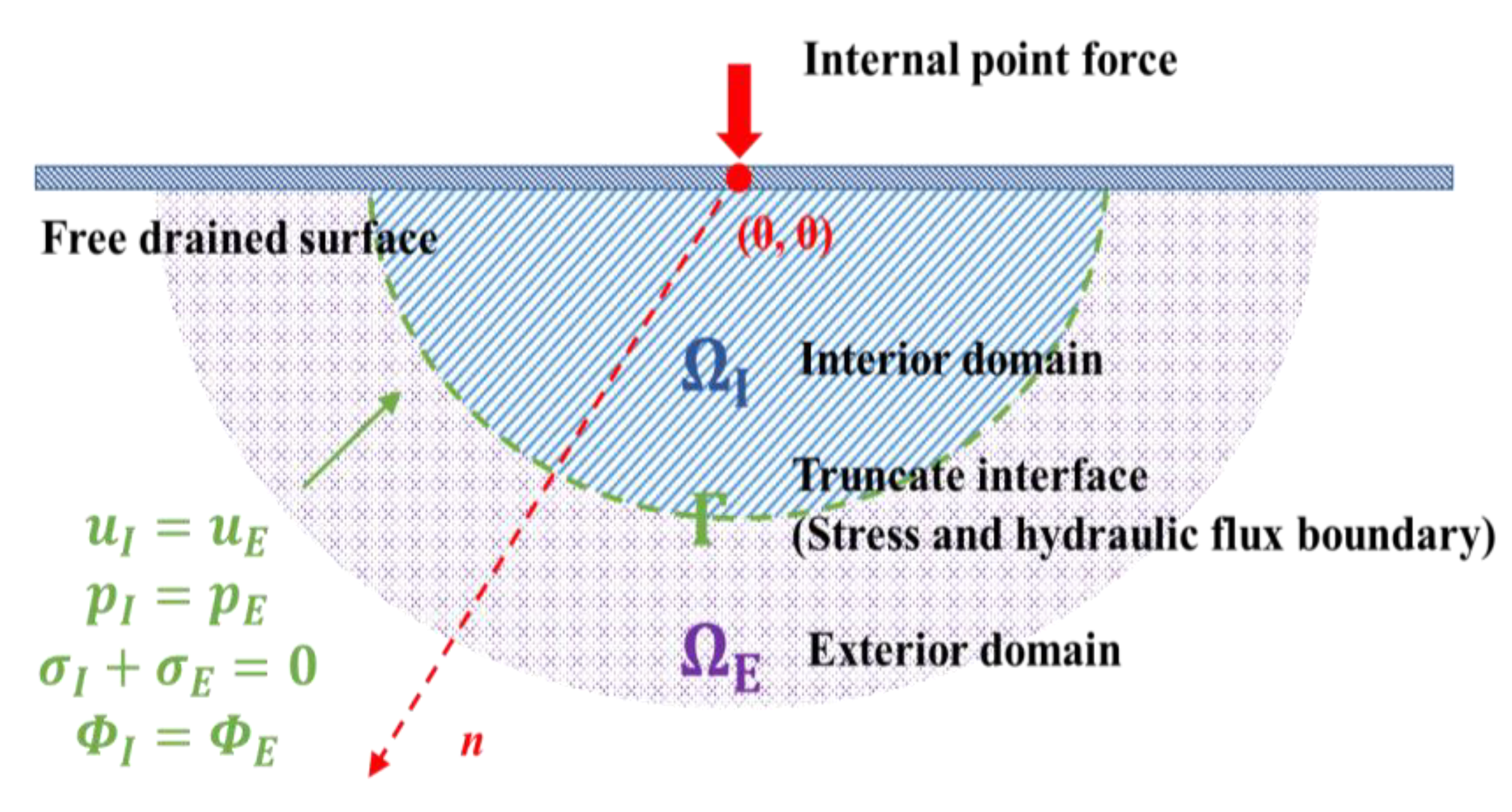
Figure 2.
One-dimensional model of fluid-saturated porous media.
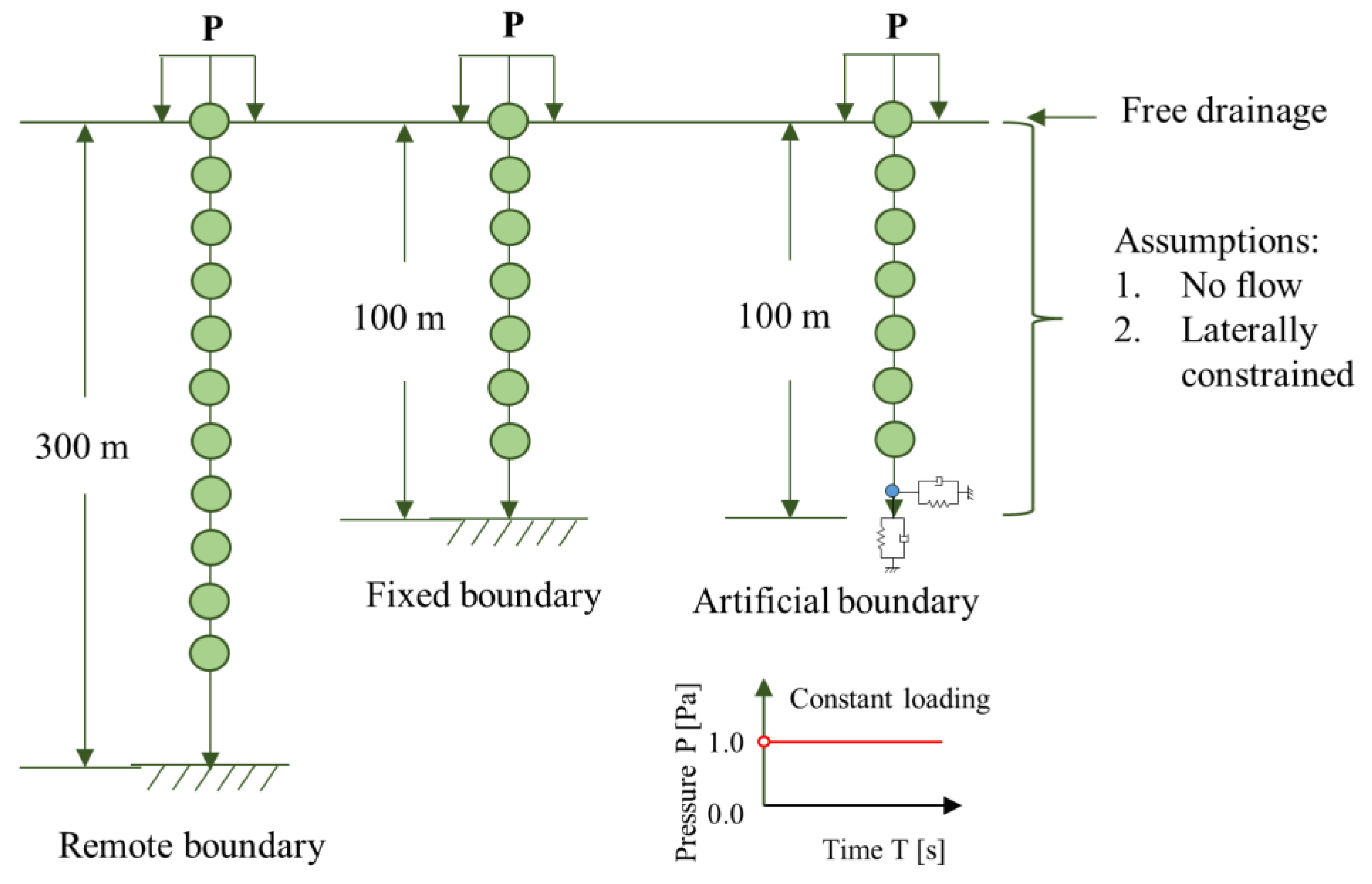
Figure 3.
Vertical displacement and pore pressure time histories of one-dimensional saturated soil model.
Figure 3.
Vertical displacement and pore pressure time histories of one-dimensional saturated soil model.
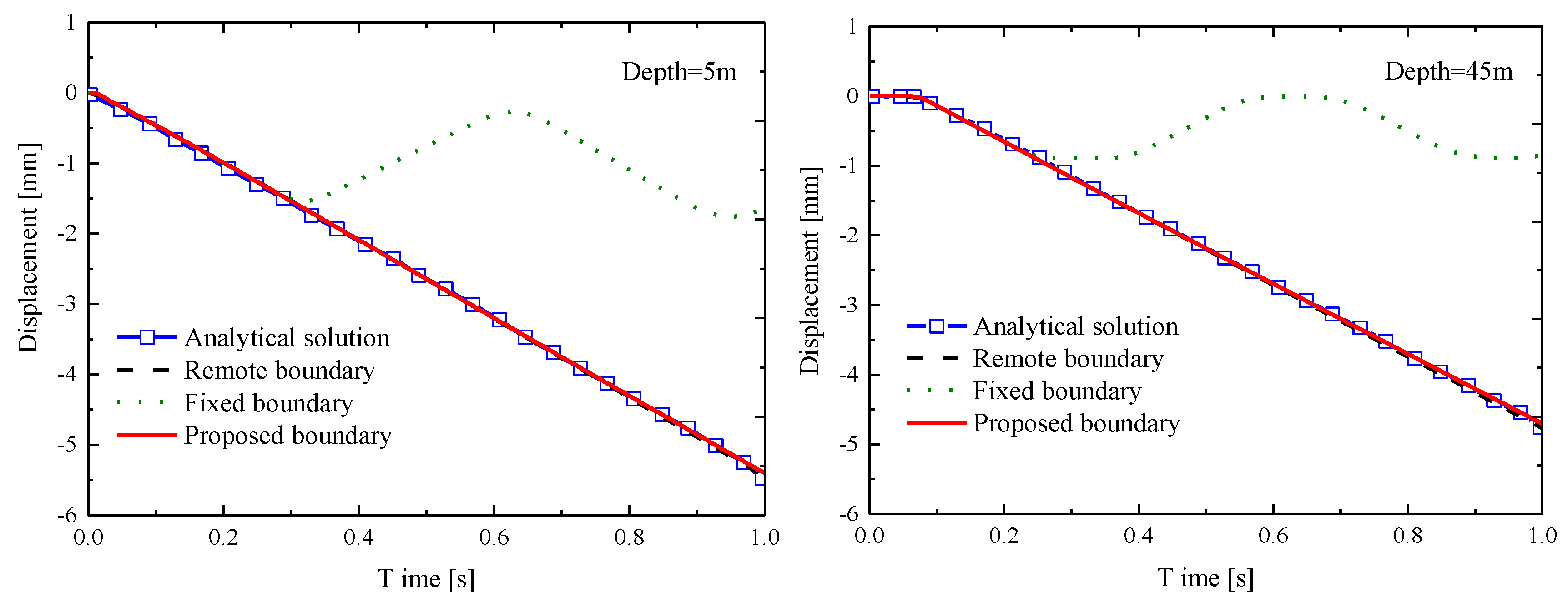

Figure 4.
Two-dimensional saturated soil model under sine loading: (a) Model with remote and fixed boundaries; (b) Model with viscous–spring boundaries.
Figure 4.
Two-dimensional saturated soil model under sine loading: (a) Model with remote and fixed boundaries; (b) Model with viscous–spring boundaries.
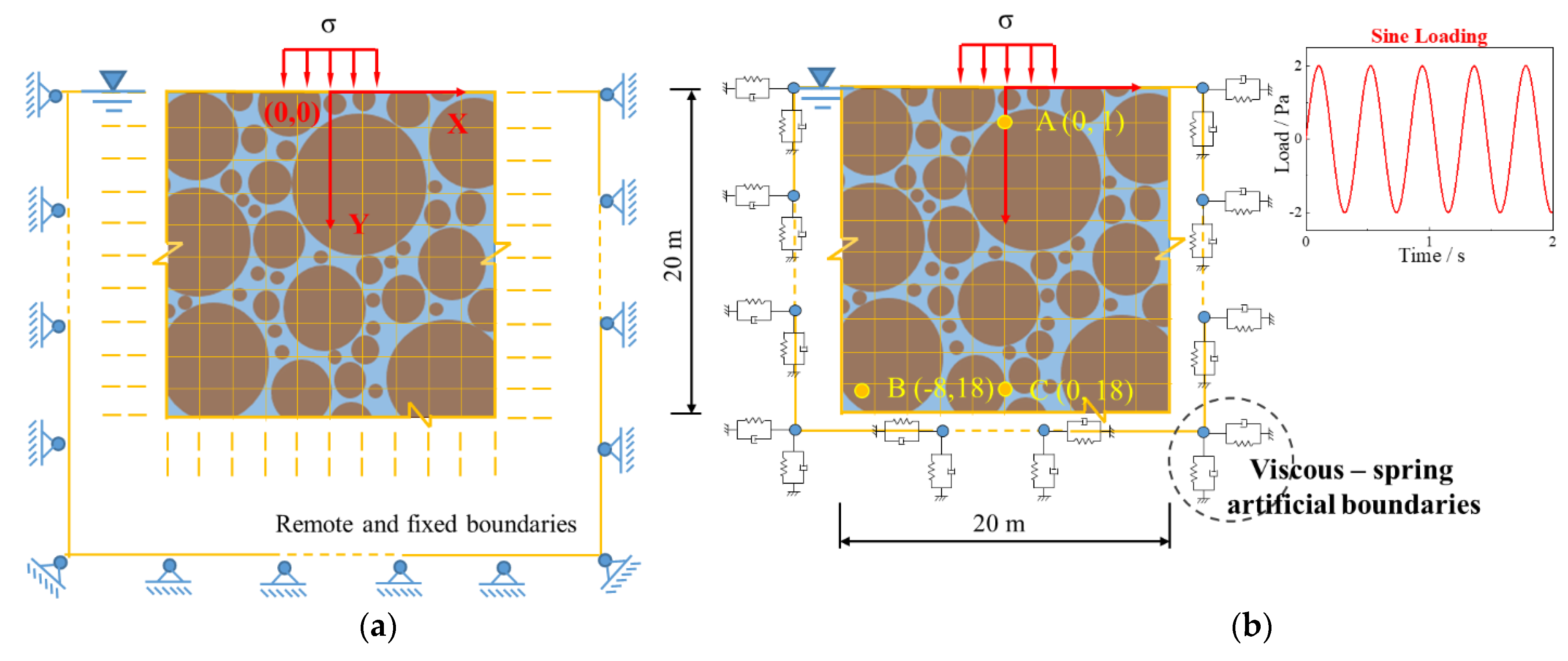
Figure 5.
Vertical displacement and pore pressure time histories of the two-dimensional model with different boundaries [51].
Figure 5.
Vertical displacement and pore pressure time histories of the two-dimensional model with different boundaries [51].
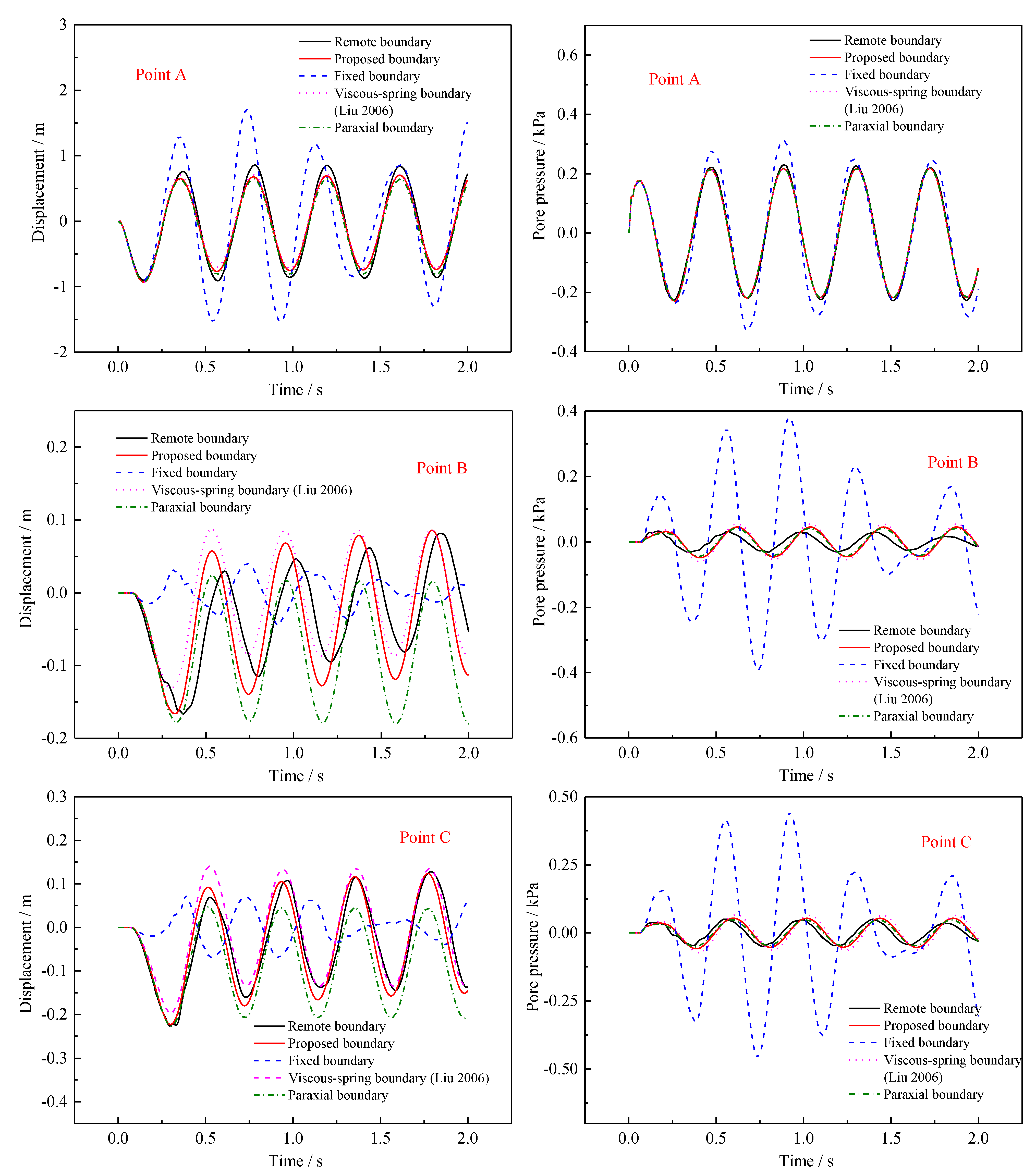
Figure 6.
Comparison of computational time [51].
Figure 6.
Comparison of computational time [51].
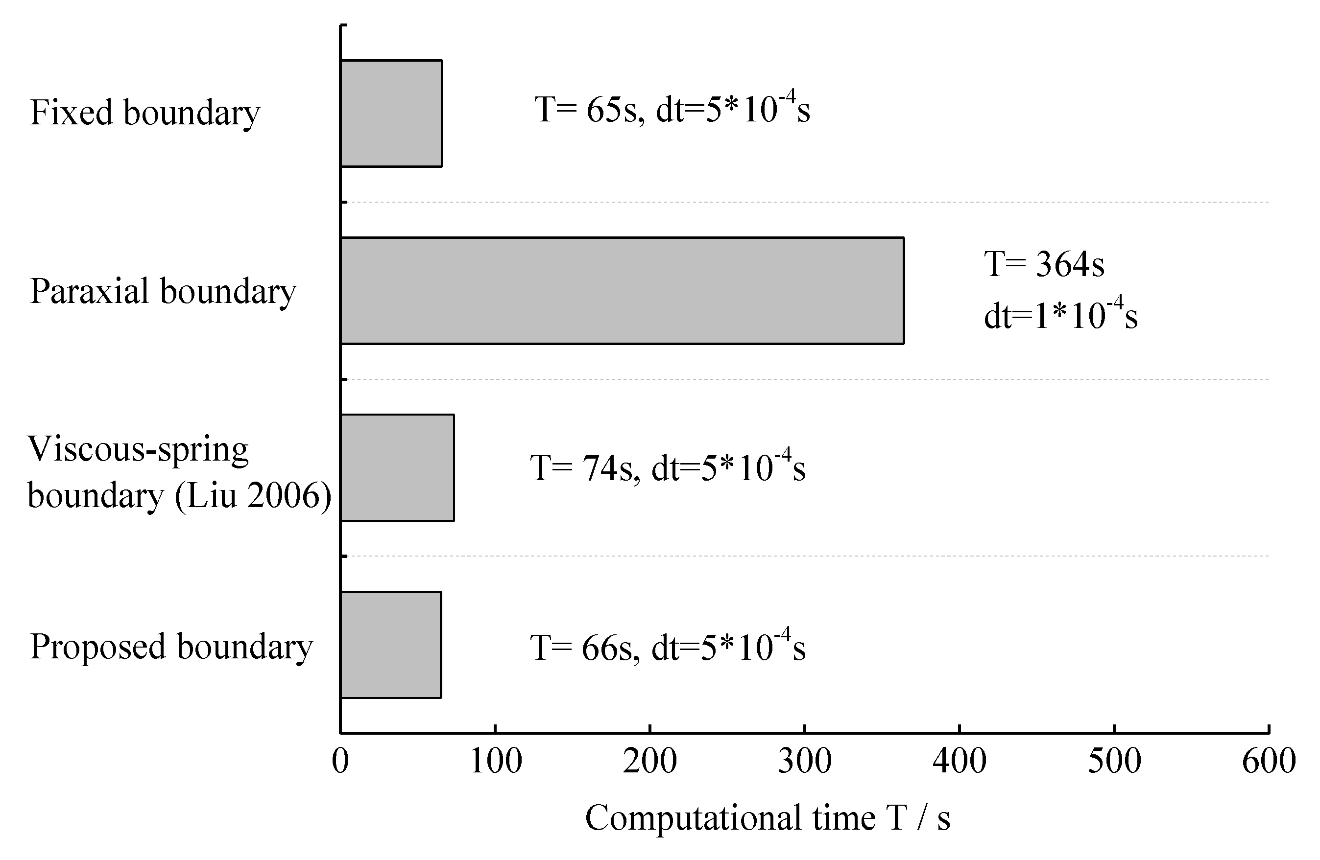
Figure 7.
Computational model under impulsive loading.

Figure 8.
Comparison of displacement at different time.

Figure 9.
Comparison of pore pressure at different time.

Table 1.
Material parameters of the linear elastic saturated soil.
| Parameter | Value | ||
| ES | 3000 Pa | Young’s modulus | |
| R | 0.306 kg/m3 | Density of two-phase media | |
| ρf | 0.2977 kg/m3 | Density of pore fluid | |
| np | 0.333 | Porosity | |
| C | 0.2 | Poisson’s ratio | |
| kf | 0.004883 m3s/kg | Dynamic permeability coefficient | |
| L | 833.3 Pa | Lame constant | |
| G | 1250 Pa | Modulus of shear | |
| Material Number | Value 1 | Value 2 | |
| Kf | 0.3999 × 10⁵ Pa | 0.6106 × 10⁵ Pa | Pore fluid volume modulus |
| Ks | ∞ | 0.5005 × 10⁴ Pa | Solid-phase soil skeleton volume modulus |
| Qb | 0.1201 × 10⁶ Pa | 0.1385 × 10⁵ Pa | Pore fluid compressibility coefficient |
| Wave Velocity | |||
| Actual Wave Velocity | Material No. | ||
| 1 | 2 | ||
| Cp | 635.12 m/s | 176.15 m/s | P wave velocity |
| Cs | 63.92 m/s | 63.92 m/s | S wave velocity |
Publisher’s Note: MDPI stays neutral with regard to jurisdictional claims in published maps and institutional affiliations. |
© 2022 by the authors. Licensee MDPI, Basel, Switzerland. This article is an open access article distributed under the terms and conditions of the Creative Commons Attribution (CC BY) license (https://creativecommons.org/licenses/by/4.0/).
Share and Cite
MDPI and ACS Style
Song, J.; Wang, F.; Jia, K.; Shen, H. A Time-Domain Artificial Boundary for Near-Field Wave Problem of Fluid Saturated Porous Media. Math. Comput. Appl. 2022, 27, 71. https://doi.org/10.3390/mca27040071
AMA Style
Song J, Wang F, Jia K, Shen H. A Time-Domain Artificial Boundary for Near-Field Wave Problem of Fluid Saturated Porous Media. Mathematical and Computational Applications. 2022; 27(4):71. https://doi.org/10.3390/mca27040071
Chicago/Turabian StyleSong, Jia, Fujie Wang, Kemin Jia, and Haohao Shen. 2022. "A Time-Domain Artificial Boundary for Near-Field Wave Problem of Fluid Saturated Porous Media" Mathematical and Computational Applications 27, no. 4: 71. https://doi.org/10.3390/mca27040071