
Developing a Robust Bioventing Model

School of Engineering, University of Guelph, Guelph, ON N1G 2W1, Canada
*
Author to whom correspondence should be addressed.
Math. Comput. Appl. 2023, 28(3), 76; https://doi.org/10.3390/mca28030076
Submission received: 16 May 2023
/
Revised: 12 June 2023
/
Accepted: 13 June 2023
/
Published: 16 June 2023
(This article belongs to the Topic Mathematical Modeling)
Abstract
:Bioventing is a widely recognized technique for the remediation of petroleum hydrocarbon-contaminated soil. In this study, the objective was to identify an optimal mathematical model that balances accuracy and ease of implementation. A comprehensive review of various models developed for bioventing was conducted wherein the advantages and disadvantages of each model were evaluated and compared regarding the different numerical methods used to solve relevant bioventing equations. After investigating the various assumptions and methods from the literature, an improved foundational bioventing model was developed that characterizes gas flow in unsaturated zones where water and non-aqueous phase liquid (NAPL) are present and immobile, accounting for interphase mass transfer and biodegradation, incorporating soil properties through a rate constant correlation. The proposed model was solved using the finite volume method in OpenFOAM, an independent dimensional open-source coding toolbox. The preliminary simulation results of a simple case indicate good agreement with the exact analytical solution of the same equations. This improved bioventing model has the potential to enhance predictions of the remediation process and support the development of efficient remediation strategies for petroleum hydrocarbon-contaminated soil.
1. Introduction
Petroleum hydrocarbons as soil contaminants endanger human health because of their potential to migrate from contaminated soil into groundwater. Therefore, it is crucial to understand how to remediate petroleum hydrocarbons-contaminated sites. Soil vapor extraction (SVE) is a popular in situ remediation approach, but it faces a tailing issue. Tailing increases mass transfer resistance, which in turn increases the clean-up time. Additionally, tailing keeps contaminant concentrations higher than the clean-up standard. Substituting SVE with an appropriate bioremediation method can eliminate these drawbacks [1]. Bioventing is usually an appropriate alternative to implement following SVE since the physical system is the same. The main difference is that nutrients are added to stimulate the microbial population and the air flow is reduced to minimize volatilization.
Bioventing (BV) is an in situ method that can economically clean up motor oil-, diesel fuel-, jet fuel-, and gasoline-contaminated soils and overcome the tailing effects caused by the SVE process [2]. Bioventing is a biological degradation technique where native aerobic microorganisms are stimulated by adding oxygen and nutrients (phosphorus and nitrogen) to bioremediate petroleum hydrocarbons [3].
The utilization of numerical simulation models has been proposed as a methodology for synthesizing laboratory-scale processes with the intricacies inherent in field settings. These models have been advanced as a means of investigating and comprehending the dynamics within BV systems. It is important to note that existing simulation models applicable to BV systems are diverse in their scope and the processes they consider [4]. Many modeling studies have been conducted to describe various aspects of bioventing and SVE systems.
Simulation models that are limited to analyzing the behavior of gas flow have been employed in the examination of pneumatic pump tests [5,6] and in the evaluation and design of SVE and BV systems [7,8]. A more complex group of models integrates analytical or numerical transport solutions with single-phase gas flow solutions [9,10]. Additionally, there are models that incorporate multiphase flow in porous media [11], the simulation of nonequilibrium interphase mass transfer and heat transfer in subsurface [12], and the inclusion of biodegradation processes [4,13,14]. Among these, the most sophisticated are those of McClure and Sleep [13] and Rathfelder et al. [4].
However, it should be noted that each of these models possess limitations in terms of their general applicability to field problems or lack of proper assumptions for developing a robust tool with reasonable computational cost for bioventing simulation. Accordingly, a literature review is conducted to investigate bioventing models’ applicability and limitations, with the aim of highlighting the importance of a new inclusive mixed model based on appropriate assumptions.
McClure and Sleep [13] developed a 2D model for bioventing using a finite difference method. The equilibrium interphase mass transfer incorporated with three-phase (gas–organic–water) flow and the dispersive transportation of oxygen, carbon dioxide, and organic components were considered in the model. The model included the consumption of components and oxygen, microorganisms’ growth, and the carbon dioxide produced due to their activation. The Dual Monod method was applied to simulate the limitations of biodegradation caused by oxygen and substrate availability. The results of the simulation showed that location and gas flow rates were the key parameters affecting the efficiency of the bioventing technique. The model is comprehensive in its consideration of several factors related to bioventing; however, the inclusion of all three phases as mobile phases necessitates a significant computational cost. Furthermore, utilizing the finite difference method to solve the problem has the disadvantage of being extremely sensitive to the size of the grid, which must be kept relatively small to obtain accurate results. As is discussed in next section, the finite difference method may not be suitable for addressing complex geometries or certain types of boundary conditions.
Rathfelder et al. [4] developed a 2D model (MISER) to simulate soil vapor extraction and bioventing by considering combined physical, chemical, and biological phenomena. The governing equations included two-phase flow, multi-component compositional transport, and non-equilibrium interphase mass transfer. MISER is considered the most sophisticated model proposed for SVE and bioventing. An aerobic biodegradation process was studied. The model was solved with the Galerkin finite element method using linear triangular elements. The mass transfer of the gas stream controlled the bioventing efficiency; a higher efficiency was achieved with an optimum supply rate of both substrate and oxygen. The model contained some assumptions which impacted the accuracy, such as the neglect of macroscopic diffusive transport within organic and solid phases. In addition, the mass transfer resistance was only considered within the aqueous phase, as was the biodegradation process [4]. MISER is the most complex and comprehensive model proposed for the simulation of both SVE and bioventing in saturated and unsaturated soil. This model is dimensionally dependent and unable to simulate 3D geometries. The complexity inherent in the model results in significant difficulties in terms of numerical solutions and the computational cost associated with simulation. The Galerkin finite element method, which is utilized as the main numerical solution method in MISER, has a limitation in effectively addressing convective-dominated problems, leading to oscillations in the results. Additionally, the source code package of MISER is not intuitive and is challenging to implement, coupled with a high computational cost associated with simulation in cases of complex geometries.
Schwarze et al. [15] modeled bioventing and included horizontal venting wells to describe the flow field of pressurized air. Biodegradation was not incorporated in the model as the purpose of the model was to assess the physical behavior of airfields in soil. The governing flow equations in the porous media were discretized using the finite volume method. The heterogeneity of the soil, as well as permeability variations, were considered in the simulation. However, random permeability variations and pressure losses of the air were excluded. The model developed by Schwarze et al. [15] appropriately accounts for relevant assumptions to accurately depict the gas flow dynamics in bioventing. However, it should be noted that the biodegradation reaction was not incorporated, as the objective of the research was to examine the gas flow in unsaturated soil rather than to predict the duration of the biodegradation process.
Sui et al. [14,16] presented a bioventing model to remediate trichloroethylene (TCE) and toluene contaminants from soil. The conditions considered in the model included the non-equilibrium interphase mass transfer, multicomponent flow, and aerobic biodegradation. An upstream-weighted multiple cell balance method and operator splitting method (OS) were applied to solve the model. A key parameter affecting contaminant distribution was the air injection rate; in the late stages of the bioventing technique, a lower flow rate was found to be more suitable. A total TCE remediation rate of 95% was achieved. Although the heterogeneity of the soil density and porosity was considered in the model, some assumptions were simplified so the accuracy decreased. The assumptions were as follows: diffusive and convective transport was assumed only in the vapor phase; the aqueous phase and NAPLs were considered immobile; sorption between the solid and gas phases was neglected; and the biodegradation was assumed to occur only within the aqueous phase.
Fernández et al. [17] developed a kinetic model for the bioremediation process of a diesel-polluted clayey soil. Mass transfer phenomena, Monod kinetics, and hydrocarbon dispersal among solid, water, non-aqueous liquid, and air phases were simultaneously modeled. The system was considered a completely closed batch reactor as the fluid flow was not incorporated in the model. The simulation results were validated using the Pearson correlation coefficient and were in good agreement with previous experimental works. The following assumptions were considered to expand the mathematical model: the system was considered closed; and the diesel contaminants were assumed to be present in all the phases. The microorganisms were homogeneously dispersed in the aqueous phase after inoculation and had access to the contaminants of the other phases. Mass transfer coefficients and kinetics parameters were estimated using the model.
Huang and Goltz [18] analytically solved the SVE equations, which incorporate terms such as mechanical dispersion, advection, molecular diffusion, and rate-limited transfer of contaminants in the form of dissolved, absorbed, and separate phases into the gas phase, by utilizing the Laplace transform with respect to time. The solutions were represented in the Laplace domain using confluent hypergeometric functions, which were subsequently inverted numerically to obtain the temporal and spatial concentration distribution of contaminants in the soil vapor extraction well. The study found that while molecular diffusion of the gas phase did not significantly impact the contaminant concentrations at extraction well, it did affect the spatial distribution of concentrations [18]. These analytical solutions provide a useful tool for designing SVE remediation strategies and verifying the performance of numerical models used to simulate SVE systems. Additionally, the model allows for the inclusion of a decay rate of contaminants as a first-order equation, enabling the modeling of a simplified form of bioventing by adjusting operation parameters such as concentration, air flow rate, and geometry. One limitation of this study is that it does not account for variations in phase saturations and assumes that the gas flow is in a steady state and unchanging throughout the duration of the study across all grid points. Another major limitation is that the analytical solution is in 1D and there is no option to solve 2D or 3D cases.
Many of the physical, biological, and chemical phenomena associated with bioventing are complex, so proposing a comprehensive bioventing model will be complicated. In addition, the structure and degree of soil heterogeneities which affect biodegradation are also challenging. Moreover, the distribution of some parameters such as water content in the field is non-uniform and not clear which imparts the metabolic capability and distribution of microorganisms in the field [19]. To develop a robust tool for predicting bioventing closure time, it is crucial to enhance the existing mixed models through the incorporation of multiphase fluid flow in porous media, the dynamics of the gas phase, interphase mass transfer mechanisms such as sorption, and biodegradation kinetics, in addition to accounting for soil properties and heterogeneity. By combining assumptions that are based on real-world bioventing systems, and reducing complexity and computational expense, this approach facilitates the creation of a more reliable tool for bioventing.
The study proposes an improved mixed model for industrial bioventing in vadose zones that considers gas phase flow in soil in the presence of immobile aqueous and NAPL phases, component transport in the phases, and biodegradation in the aqueous phase. The model incorporates soil properties through a rate constant correlation and soil heterogeneity to provide a reliable tool for predicting unsaturated bioventing closure time. Furthermore, the model can be utilized to investigate soil vapor extraction, gas flow dynamics in soil, and the effectiveness of injection and extraction wells, as well as to explore the effects of soil heterogeneity and variations in gas permeability. The proposed model is numerically implemented in OpenFOAM using the finite volume method and is adaptable to various geometries and boundary conditions in 3D simulation. The selection of the main assumptions for model development is discussed in detail in the model development section to enhance the model’s prediction accuracy while minimizing computational costs.
2. Different Mathematical Solutions of Bioventing Equations
The selection of an appropriate mathematical solution for a bioventing model is crucial for achieving accurate results within a reasonable computational time. This is particularly important when accounting for key elements of the bioventing process and aligning the model’s assumptions with specific research objectives. Various methods have been used in the past to solve these equations. Some of the key methods that may be discussed include analytical solutions, numerical solutions, and hybrid solutions.
Numerous studies have been conducted on the analytical solutions of bioventing equations, with a focus on resolving coupled component transport and reaction equations [18,20,21,22,23]. However, it should be noted that analytical methods have a solution constraint when applied to models that incorporate multiple sets of equations such as phase flow, component transport, mass transfer, and biodegradation equations. This limitation necessitates the utilization of numerical methods or a combination of numerical and analytical methods (hybrid) to fully capture the complexity of the system under investigation.
Different numerical methods, including finite difference (FD), finite element (FE), and finite volume (FV), are commonly used to solve equations related to flow and transport in porous media [24]. Each method has its own advantages and disadvantages, and it is crucial to consider these factors when selecting the most appropriate method for a particular study, considering the nature of the equations, goal of the research, and availability of necessary tools.
The FDM (finite difference method) is a widely used and versatile method for solving bioventing numerical model equations [13,16,25], but it is not without its limitations. It is an efficient method that can be used to solve a wide range of problems. One of the main advantages of FDM is its simplicity and ease of implementation. The method involves dividing the domain of interest into a grid of discrete points and approximating the derivatives in the equations using the values at these points. This makes it straightforward to implement and can be applied to a wide range of equations. FDM, in the same way as any other approximation, has certain limitations, including oscillations and diffusion, particularly at discontinuous points. Additionally, FDM may encounter issues with conserving mass since it is mass conservative only when the grid spacing goes to zero and may have difficulty handling irregular shapes [26,27].
On the other hand, FE is a complex numerical method which has been widely used to solve the equations of flow and transport in porous media for decades [14,28,29]. In some complex cases such as coupled flow and transport in porous media including interphase mass transfer and biodegradation, using FEM provides the option of combining different kinds of functions that approximate the solution of each equation within each element. This is referred to as mixed formulation [4]. Compared to FDM, the FE method is quite capable of handling complex geometries and unstructured meshes [30].
The main disadvantage of the classic FE method is that it is not mass conservative, which might cause difficulties in the convergence of the final code. Numerous studies have been conducted to improve classic FE and render it mass conservative [31]. Regarding mass conservation, volume discretization approaches of FEM and FDM are more beneficial when compared to ordinary FE techniques. These methods are locally conservative, contrary to classic FE approaches. Although mixed FE approaches are locally mass conservative, they are not efficient. In nonlinear cases, which include large grid alterations, local mass conservation is significant to avoid considerable errors [12].
The finite volume method (FVM) is a numerical method which converts partial differential equations illustrating conservation laws on differential volumes to discrete algebraic equations expanding on finite volumes, cells, or elements. To solve partial differential equations using FVM, first the domain should be discretized, similar to the first step in the finite element or finite difference methods. Then the geometric domain is discretized into finite volumes or elements which are not overlapped in the FVM technique. The partial differential equations are integrated over each discrete volume, and then converted to the set of algebraic equations. After that, the dependent variables are computed for each element, solving the set of algebraic equations. Some terms of conservation equations are transformed into face fluxes and, therefore, are assessed at the finite-volume faces [32].
The FVM is strictly conservative, since the flux entering a volume is equal to the flux exiting the neighbouring volume. Therefore, FVM is preferable in computational fluid dynamics (CFD) due to this intrinsic conservation feature [26]. The FVM is even applicable on unstructured polygonal meshes which is a significant advantage of this method. The FVM is easily applicable to various boundary conditions because the computations of unknown variables are carried out at the centroids of volume elements instead of their boundaries [15,32,33]. Considering the above-mentioned attributes of the FV approach, it is a useful method to numerically simulate complex systems involving mass transfer, component transport, and fluid flow in porous media.
3. Proposed Model Development and Implementation
The literature shows that bioventing in vadose zones incorporates three main aspects including fluid flow in porous media, component transport, and biodegradation reactions. The selection of assumptions regarding each of these aspects is crucial to develop a robust simulation tool balancing adequate results, complexity, and computational cost.
3.1. Fluid Flow (Convection) in Unsaturated Bioventing
Considering three present phases in unsaturated bioventing, phase flow in soil has been modeled as three-phase flow [13], two-phase flow (gas and aqueous) with the NAPL phase kept immobile [4], and one-phase flow (gas) in the presence of immobile aqueous and NAPL phases [14,15]. The reason for considering mobile liquid phases is to either account for saturated soil or high water or NAPL saturation in unsaturated zones, which are not applicable for bioventing in vadose zones. According to the literature, the water content range for optimal microorganism activity is 5–20 wt.%. Shewfelt et al. [34] showed that optimum bioventing conditions were 18 wt.% soil water content. Under conditions of low soil moisture content, this corresponds to 50–70% of soil’s water-holding capacity where capillarity confines water to smaller void spaces, resulting in the gas phase being continuous and enabling gas transport driven by potential gradients. However, when the water content is high, gases become confined to large void spaces in the form of bubbles, with the aqueous phase being continuous. In such conditions, convective transport of the gas phase is not anticipated [35].
High water content in soil is a limitation to microorganisms’ activity which is why moisture content must be kept in an optimally low range [34,36,37]. Additionally, bioventing is a common alternative for low contamination concentrations and is applied after SVE to overcome the tailing effect [1]. Considering these limitations, aqueous and NAPL phases are not continuous in vadose-zone bioventing, and the only convective phase is gas phase. However, the presence of liquid phase affects the gas flow regime and must be incorporated into the model through gas-phase relative permeability which is a function of aqueous-phase saturation [38]. This leads to a flow equation incorporating advection, dispersion, and diffusion in the gas phase, which provides gas-phase pressure and velocity distributions through the system’s geometry. Changes in saturations of liquid phases are due to interphase mass transfer and biodegradation rates in the aqueous phase (Equation (1)).
is soil porosity. is gas-phase saturation in soil. and represent gas density and viscosity, respectively. is gas-phase relative permeability. stands for gas pressure and is gravity acceleration. is the summation of mass transfer rates from other phases to the gas phase which are first-order Fick’s equations and is the source term in the gas phase.
The interphase mass transfer of component k to/from gas phase is described with a linear driving force expression (Equation (2)) and the summation of mass transfer rates to/from the gas phase to other phases is presented as Equation (3).
stands for the summation of mass transfer rates of component I from other phases to the gas phase which are first-order Fick’s equations. is component i’s mass transfer constant between the gas phase and the phase. is the equilibrium concentration of component i between the gas phase and the phase. is the concentration of component i in the gas phase.
Equations describing phase mass balances for the aqueous phase (Equation (4)) and the NAPL phase (Equation (5)) are presented as follows:
is the contaminant biodegradation rate in the aqueous phase.
3.2. Component Transport
A general macroscopic equation governing the transport of components in the gas phase in unsaturated soil is based on Darcy’s velocity [4] and is described in Equation (6). Dispersion and diffusion are included in the model. Interphase mass transfer is considered in two selective options, rate-limited mass transfer and equilibrium interphase partitioning.
D and are the dispersion coefficient and Darcy’s velocity of the gas phase, respectively.
Component i’s mass balances for aqueous and NAPL phases are described in Equations (7) and (8), respectively. Biodegradation is assumed to occur for each contaminant component i in the aqueous phase.
3.3. Biodegradation
Microbial activity is the main concept of contaminant reduction in bioventing. An adequate prediction of bioreaction is crucial to predict the closure time [39]. Different kinetics for biodegradation have been employed in the literature including Monod kinetics and first-order kinetics. In Monod-type kinetics, the rate of reaction is determined by the concentration of the limiting nutrient. Specifically, the reaction rate increases as the concentration of the limiting nutrient increases until it reaches a maximum value called the maximum specific growth rate. At higher nutrient concentrations, the reaction rate levels off and eventually reaches a plateau [39]. In other words, this approach assumes that the conversion of contaminant into biomass is not instantaneous and microbial activity may be limited by the diffusional mass transfer resistance.
Incorporating Monod-type kinetics requires a set of initial values and constant parameters to import into the model [4]. On the other hand, first-order kinetics are incorporated in models and assume that all reaction components including nutrients, oxygen, and microorganisms are available and not limited and the bioreaction takes place instantaneously [39]. The proposed model includes first-order kinetics due to the surplus of oxygen and nutrients supplied during industrial bioventing [40]. The bioreaction is constrained by microbes’ access to the contaminant, which is represented in the model through the rate-limited mass transfer of the contaminant to the aqueous phase and used to calibrate the model against experimental data.
where C is the concentration of contaminant in soil (mg/kg); C0 is the initial concentration of contaminant in soil (mg/kg); k is the decay rate (day−1); and t is time (day).
Additionally, the model employs a biodegradation rate constant correlation to integrate soil properties into the model. A two-stage rate constant correlation derived by Khan and Zytner [41] is presented in Equations (10) and (11).
PDB = initial population of petroleum-degrading microorganisms in soil, log colony-forming units (CFU/g of soil);
Sand = sand content, %;
Clay = clay content, %;
SW = soil water content, %;
OM = organic matter content, %.
4. Model Implementation
The equations are mathematically solved using FVM in OpenFOAM which is an open-source coding toolbox for computational fluid dynamics (CFD) analysis. The utilization of OpenFOAM allows for the deployment of simulation on parallel computers and provides the advantage of unlimited customization through the extension of solvers, utilities, and libraries, with the prerequisite knowledge of the underlying method, physics, and programming techniques. The software is code-based, utilizing the C++ programming language, resulting in a highly flexible modeling environment, facilitating ease of adjustment of parameters and equations, as necessary.
Another significant benefit of this model is being dimensionally independent. OpenFOAM has automatic discretization of equations. This allows any solver to be used on 1D, 2D, or 3D meshes and models can be run by imposing user-defined meshes and geometry. Meshes and geometry can be created in OpenFOAM or in other software such as Fluent.
Simple Case Simulation
To show the efficiency of the proposed model and FVM in OpenFOAM, a simple case is simulated considering steady-state gas flow (constant velocity) and component mass balance in all three phases. The model’s solution was compared against the analytical solution by Huang and Goltz [18].
Huang and Goltz [18] proposed an analytical solution to model a SVE system. Considering the similar soil physics of SVE and bioventing systems, by adding a first-order kinetics term to the aqueous-phase component mass balance equation, the simulation was performed for bioventing.
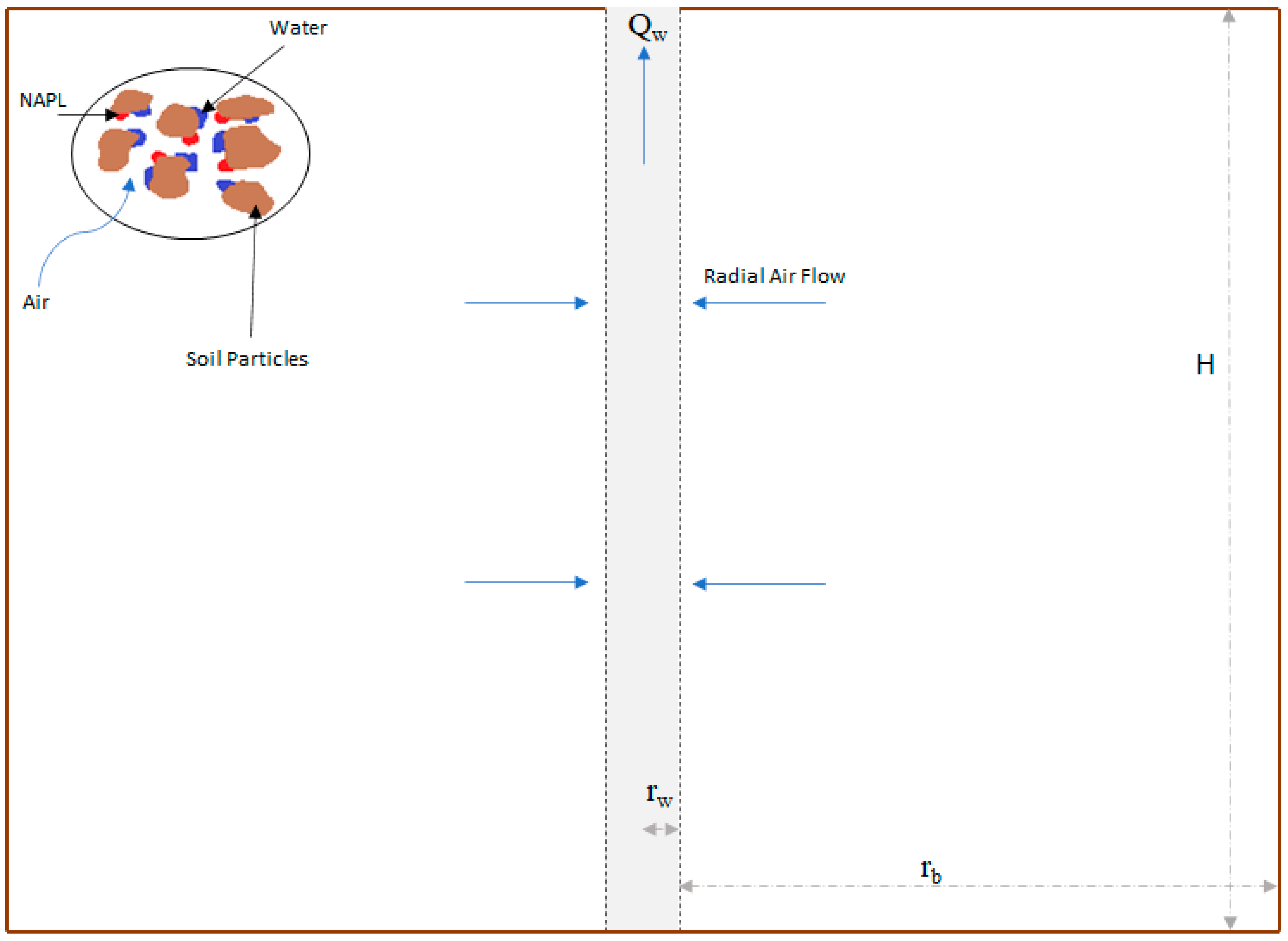
A conceptual model of the application of SVE/bioventing in a contaminated vadose zone is presented in Figure 1 based on the work of Huang and Goltz [18]. An extraction well is located on the left-hand side of the mesh and air is extracted radially through this well. Contamination concentration in soil is homogeneous in an area with radius 50 m and depth of 3 m and the change in gas-phase concentration during the process is only radial (Figure 1).
The vadose zone is composed of voids filled with air, water, and NAPL, where volatilized contaminant is extracted through a fully screened well. Meanwhile, dissolved and NAPL-phase contaminants volatilize into the gas phase. To mathematically describe the conceptual model, several assumptions were made. A steady, radially convergent gas flow field is induced by the extraction well, where water and NAPL phases are immobile, the transport of volatilized contaminants in the vadose zone is governed by advection, dispersion, and molecular diffusion, contaminant mass transfer between phases can be described by first-order kinetics, and first-order biodegradation of contaminant occurs in the aqueous phase.
Another assumption made by Huang and Goltz [18] is that saturation of NAPLs is low; therefore, NAPL desaturation does not significantly affect gas- and water-phase saturations, which are assumed to be constant. However, in the FVM model, changes in the saturations of all the phases are considered and for the immobile phases (aqueous phase and NAPL phase), changes in saturations are only due to mass transfer and biodegradation (in the aqueous phase). In this case, a simple form of contaminant transport in bioventing was simulated and the code was incorporated in a 2D mesh in which the change in gas-phase concentration is radial only (1D).
5. Results and Discussion
When designing and implementing a bioventing process for a hydrocarbon-contaminated site, accurately predicting the closure time is of paramount importance for site owners and consultants. However, current commercial software tools for this purpose have limitations when simulating different cases. The presented model aims to provide a robust solution to these limitations by satisfying the following criteria:
- Offering robustness and low computational cost by allowing for simulation of simple geometries on a personal computer;
- Supporting any type of geometry and boundary conditions, as well as the option to run complex simulations on parallel computing cores and cloud-based systems;
- Incorporating all relevant aspects of bioventing, including fluid flow in porous media in the presence of three phases, biodegradation kinetics, and component transport;
- Incorporating soil properties through a biodegradation constant correlation that considers the effect of different soil types;
- Providing flexibility to run simulations in 1D, 2D, and 3D;
- Accounting for soil heterogeneity in complex systems, including different soil layers, variable soil permeability, and changes in soil moisture content;
- Accounting for the effect of aged contamination;
- The ability to simulate both SVE and bioventing.
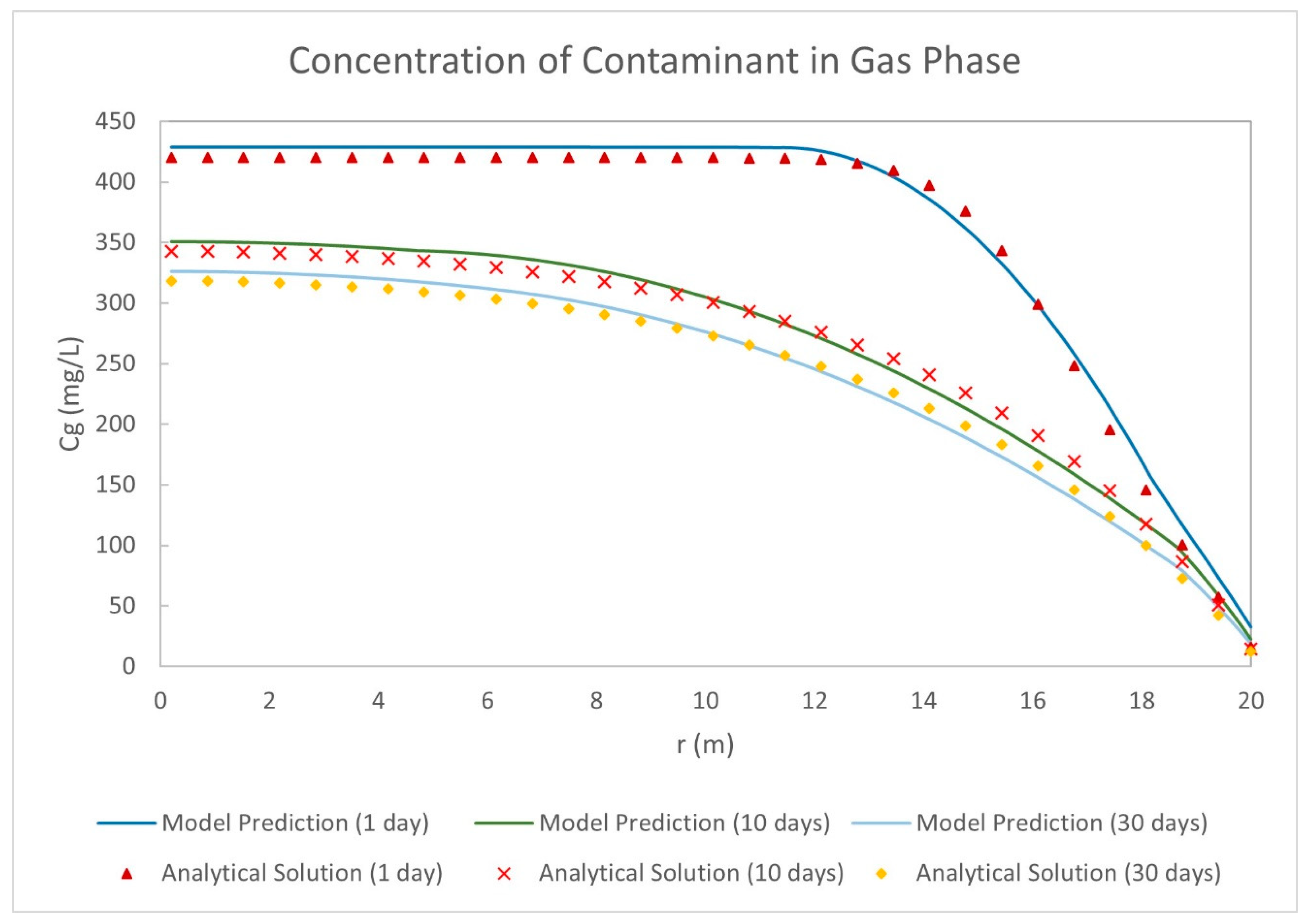
The model is simulated in OpenFOAM for three separate time periods (1 day, 10 days, 30 days) to determine the concentration of contaminant present in the gas phase at 20 m (rb in Figure 1) from the extraction well. Thirty days is the duration of the experiments used to generate the calibrating data [1]. The velocity of gas flow is calculated using Darcy’s equation, and it is presumed that alterations in saturations do not influence the velocity of the gas phase in the soil. The calculated Darcy’s velocity is then utilized to assess the component transport in the gas phase, which can be used to infer the concentration profile.
The analytical results of this study are based on the research of Huang and Goltz [18]. The model equations are solved analytically by employing the Laplace transform method with respect to time. The solutions are depicted using confluent hypergeometric functions in the Laplace domain, and subsequently evaluated through a numerical Laplace inversion algorithm. These solutions enable the simulation of the spatial distribution and temporal evolution of contaminant concentrations that may arise during the operation of a SVE/bioventing well. The code is developed in MATLAB and represents the exact solution of the component transport equations by considering a steady-state constant gas velocity. Additionally, first-order kinetics are employed to represent biodegradation in the aqueous phase. All the relevant parameters and initial conditions used in both models are presented in Table 1.
Figure 2 shows good consistency in trends with respect to time and space between the analytical solution and the developed model. The slight difference between results is due to a basic assumption which is made in the analytical method. Huang and Goltz [18] assumed that the saturations of gas and aqueous phases do not change during the process which is a simplifying assumption to help develop the analytical solution. However, in the numerical FVM model, changes in saturations are accounted for and this probably caused the slight difference in results.
The standard error of regression (SER) method is used to show how precise the model’s predictions are against the results of the analytical solution using the units of the dependent variable (mg/L).
N is number of values in each set; in and jn represent values of numerical results and analytical results, respectively.
The SER value indicates how far the data points are from the regression line on average. The result shows the error for cases of 1 day, 10 days, and 30 days as 10.4 (2.48%), 8.12 (2.37%), and 6.64 (2.08 %), respectively.
In the next phase of the research, a more comprehensive simulation will be performed to validate the model using independent sets of experimental data published by Khan and Zytner [1,41] and Mosco and Zytner [42] by simulating bioventing in a larger cylindrical reactor in 3D. Furthermore, a comprehensive simulation will be conducted to analyze the impacts of soil heterogeneity and the aging of contamination on the bioventing closure time. To account for aged contaminated soil, a correlation developed by Mosco and Zytner [42] will be employed to correlate the biodegradation rate constant, which will be integrated into the model. In addition, the reactor will be modeled with various permeable layers of soil to examine the heterogeneity of the system.
6. Conclusions
The foundation of a comprehensive bioventing model was developed to accurately predict closure time. After investigating various models and their assumptions, an improved mixed model for industrial bioventing in vadose zones is proposed that considers gas-phase flow in soil, immobile aqueous and NAPL phases, component transport, and biodegradation in the aqueous phase. Soil properties are incorporated through a degradation rate constant correlation and soil heterogeneity to provide a dependable tool for forecasting unsaturated bioventing closure time.
Selecting the appropriate numerical method to solve the model needs to be capable of addressing the intricacies of equations and geometry, a crucial element in the advancement of bioventing simulation. Comparing applications of different mathematical methods shows that FVM features such as mass conservation, applicability on unstructured polygonal meshes, and ease of implementing various boundary conditions make it the best choice to solve the proposed mathematical model. OpenFOAM was selected to implement the simulation due to its ability to deploy simulations on parallel computers, unlimited customization, flexibility, and dimensionally independent nature with automatic discretization of equations. These features allow for easy adjustment of parameters and equations as necessary and the ability to use any solver on 1D, 2D or 3D mesh with user-defined meshes and geometry.
A simple form of the foundational numerical model was simulated, and the results were compared to an analytical solution presenting a good match with errors less than 2.5%, showing the accuracy of mass-conservative FVM. This success shows the potential to build on the foundation model and incorporate additional scenarios.
Author Contributions
Conceptualization, R.G.Z.; methodology, M.K.S. and R.G.Z.; software, M.K.S.; validation, M.K.S. and R.G.Z.; investigation, M.K.S. and R.G.Z.; resources, R.G.Z.; data curation, M.K.S.; writing original draft preparation, M.K.S.; writing—review and editing, R.G.Z.; visualization, M.K.S.; supervision, R.G.Z.; project administration, R.G.Z.; funding acquisition, R.G.Z. All authors have read and agreed to the published version of the manuscript.
Funding
The research was supported by the corresponding author’s Natural Science and Engineering Re-search Council (NSERC) of Canada Discovery Grant [400-913] and a University of Guelph General Purpose Research Account [070-669].
Data Availability Statement
The data presented in this study are available on request from the corresponding author. The data are not publicly available as the project is not yet completed.
Conflicts of Interest
The authors declare no conflict of interest.
References
- Khan, A.; Zytner, R.G. Degradation rates for petroleum hydrocarbons undergoing bioventing at the meso-scale. Bioremediat. J. 2013, 17, 159–172. [Google Scholar] [CrossRef]
- Eyvazi, M.J.; Zytner, R.G. A correlation to estimate the bioventing degradation rate constant. Bioremediat. J. 2009, 13, 141–153. [Google Scholar] [CrossRef]
- Nikolopoulou, M.; Kalogerakis, N. Enhanced bioremediation of crude oil utilizing lipophilic fertilizers combined with biosurfactants and molasses. Mar. Pollut. Bull. 2008, 56, 1855–1861. [Google Scholar] [CrossRef] [PubMed]
- Rathfelder, K.M.; Lang, J.R.; Abriola, L.M. A numerical model (MISER) for the simulation of coupled physical, chemical and biological processes in soil vapor extraction and bioventing systems. J. Contam. Hydrol. 2000, 43, 239–270. [Google Scholar] [CrossRef]
- Baehr, A.L.; Hult, M.F. Evaluation of unsaturated zone air permeability through pneumatic tests. Water Resour. Res. 1991, 27, 2605–2617. [Google Scholar] [CrossRef]
- Massmann, J.W.; Madden, M. Estimating air conductivity and porosity from vadose zone pumping tests. J. Environ. Eng. 1994, 120, 313–328. [Google Scholar] [CrossRef]
- Sepehr, M.; Samani, Z.A. In situ soil remediation using vapor extraction wells, development and testing of a three-dimensional finite difference model. Groundwater 1993, 31, 425–436. [Google Scholar] [CrossRef]
- Mohr, D.H.; Merz, P.H. Application of a 2D air flow model to soil vapor extraction and bioventing case studies. Groundwater 1995, 33, 433–444. [Google Scholar] [CrossRef]
- Zaidel, J.; Russo, D. Analytical models of steady state organic species transport in the vadose zone with kinetically controlled volatilization and dissolution. Water Resour. Res. 1993, 29, 3343–3356. [Google Scholar] [CrossRef]
- Weber, A.Z.; Newman, J. Modeling gas-phase flow in porous media. Int. Commun. Heat Mass Transf. 2005, 32, 855–860. [Google Scholar] [CrossRef]
- Horgue, P.; Soulaine, C.; Franc, J.; Guibert, R.; Debenest, G. An open-source toolbox for multiphase flow in porous media. Comput. Phys. Commun. 2015, 187, 217–226. [Google Scholar] [CrossRef] [Green Version]
- Zyvoloski, G. FEHM: A Control Volume Finite Element Code for Simulating Subsurface Multi-Phase Multi-Fluid Heat and Mass Transfer, LAUR-07-3359; Los Alamos National Laboratory: Los Alamos, NM, USA, 2007. [Google Scholar]
- McClure, P.D.; Sleep, B.E. Simulation of bioventing for soil and ground-water remediation. J. Environ. Eng. 1996, 122, 1003–1012. [Google Scholar] [CrossRef]
- Sui, H.; Li, X. Modeling for volatilization and bioremediation of toluene-contaminated soil by bioventing. Chin. J. Chem. Eng. 2011, 19, 340–348. [Google Scholar] [CrossRef]
- Schwarze, R.; Mothes, J.; Obermeier, F.; Schreiber, H. Numerical Modeling of Soil Bioventing Processes–Fundamentals and Validation. Transp. Porous Med. 2004, 55, 257–273. [Google Scholar] [CrossRef]
- Sui, H.; Li, X.; Jiang, B. A study on cometabolic bioventing for the in-situ remediation of trichloroethylene. Environ. Geochem. Health 2006, 28, 147–152. [Google Scholar] [CrossRef]
- Fernández, E.L.; Merlo, E.M.; Mayor, L.R.; Camacho, J.V. Kinetic modelling of a diesel-polluted clayey soil bioremediation process. Sci. Total Environ. 2016, 557, 276–284. [Google Scholar] [CrossRef]
- Huang, J.; Goltz, M.N. Analytical solutions for a soil vapor extraction model that incorporates gas phase dispersion and molecular diffusion. J. Hydrol. 2017, 549, 452–460. [Google Scholar] [CrossRef]
- Rubin, H.; Rubin, E.; Schüttrumpf, H. Modeling and implementation of sustainable remediation based on bioventing. In Bioremediation and Sustainability: Research and Applications; John Wiley & Sons: Hoboken, NJ, USA, 2012; pp. 317–366. [Google Scholar] [CrossRef]
- Clement, T.P. Generalized solution to multispecies transport equations coupled with a first-order reaction network. Water Resour. Res. 2001, 37, 157–163. [Google Scholar] [CrossRef]
- Sun, Y.; Lu, X.; Petersen, J.N.; Buscheck, T.A. An analytical solution of tetrachloroethylene transport and biodegradation. Transp. Porous Media 2004, 55, 301–308. [Google Scholar] [CrossRef]
- Mieles, J.; Zhan, H. Analytical solutions of one-dimensional multispecies reactive transport in a permeable reactive barrier-aquifer system. J. Contam. Hydrol. 2012, 134, 54–68. [Google Scholar] [CrossRef]
- Veling, E.J.M. Radial transport in a porous medium with Dirichlet, Neumann and Robin-type inhomogeneous boundary values and general initial data: Analytical solution and evaluation. J. Eng. Math. 2012, 75, 173–189. [Google Scholar] [CrossRef] [Green Version]
- Pinder, G.F. Forty Years of Ground Water Modeling. Water Resour. IMPACT 2014, 16, 24–25. Available online: https://www.jstor.org/stable/wateresoimpa.16.3.0024 (accessed on 24 January 2023).
- Sleep, B.E.; Sykes, J.F. Compositional simulation of groundwater contamination by organic compounds: 1. Model development and verification. Water Resour. Res. 1993, 29, 1697–1708. [Google Scholar] [CrossRef]
- Ali, A.H.; Jaber, A.S.; Yaseen, M.T.; Rasheed, M.; Bazighifan, O.; Nofal, T.A. A comparison of finite difference and finite volume methods with numerical simulations: Burger’s equation model. Complexity 2022, 2022, 9367638. [Google Scholar] [CrossRef]
- Kaur, R.; Kumar, S.; Kukreja, V.K. Numerical approximation of generalized burger’s-Fisher and generalized burger’s-huxley equation by compact finite difference method. Adv. Math. Phys. 2021, 2021, 3346387. [Google Scholar] [CrossRef]
- Abriola, L.M.; Lang, J.R. Self-adaptive hierarchic finite element solution of the one-dimensional unsaturated flow equation. Int. J. Numer. Methods Fluids 1990, 10, 227–246. [Google Scholar] [CrossRef] [Green Version]
- Fen, C.S.; Abriola, L.M. A comparison of mathematical model formulations for organic vapor transport in porous media. Adv. Water Resour. 2004, 27, 1005–1016. [Google Scholar] [CrossRef]
- Simpson, M.J.; Clement, T.P. Comparison of finite difference and finite element solutions to the variably saturated flow equation. J. Hydrol. 2003, 270, 49–64. [Google Scholar] [CrossRef]
- Salinas, P.; Pavlidis, D.; Xie, Z.; Osman, H.; Pain, C.C.; Jackson, M.D. A discontinuous control volume finite element method for multi-phase flow in heterogeneous porous media. J. Comput. Phys. 2018, 352, 602–614. [Google Scholar] [CrossRef]
- Moukalled, F.; Mangani, L.; Darwish, M. The Finite Volume Method in Computational Fluid Dynamics: An Advanced Introduction with OpenFOAM and Matlab; Fluid Mechanics and Its Applications; Springer International Publishing: Berlin/Heidelberg, Germany, 2016. [Google Scholar]
- Shukla, A.; Singh, A.K.; Singh, P. A comparative study of finite volume method and finite difference method for convection-diffusion problem. Am. J. Comput. Appl. Math. 2011, 1, 67–73. [Google Scholar] [CrossRef]
- Shewfelt, K.; Lee, H.; Zytner, R.G. Optimization of nitrogen for bioventing of gasoline contaminated soil. J. Environ. Eng. Sci. 2005, 4, 29–42. [Google Scholar] [CrossRef]
- Tellez, C.M.; Aguilar-Aguila, A.; Arnold, R.G.; Guzman, R.Z. Fundamentals and modeling aspects of bioventing. In Fundamentals and Applications of Bioremediation; Routledge: Milton Park, UK, 1998; pp. 135–183. [Google Scholar] [CrossRef]
- King, M.M.; Kinner, N.E.; Deming, D.P.; Simonton, J.A.; Belden, L.M. Bioventing of no. 2 fuel oil: Effects of air flowrate, temperature, nutrient amendment, and acclimation. Remediat. J. 2014, 24, 47–60. [Google Scholar] [CrossRef]
- Sharma, J. Advantages and limitations of in situ methods of bioremediation. Recent Adv. Biol. Med. 2019, 5, 10941. [Google Scholar] [CrossRef] [Green Version]
- Ho, C.K.; Webb, S.W. Gas Transport in Porous Media; Springer Science & Business Media: Berlin/Heidelberg, Germany, 2006; Volume 20. [Google Scholar] [CrossRef]
- Looney, B.B.; Falta, R.W. Vadose Zone: Science and Technology Solutions; Battelle Press: Columbus, OH, USA, 2000. [Google Scholar]
- Agarry, S.; Latinwo, G.K. Biodegradation of diesel oil in soil and its enhancement by application of bioventing and amendment with brewery waste effluents as biostimulation-bioaugmentation agents. J. Ecol. Eng. 2015, 16, 82–91. [Google Scholar] [CrossRef]
- Khan, A.A.; Zytner, R.G.; Feng, Z. Establishing correlations and scale-up factor for estimating the petroleum biodegradation rate in soil. Bioremediat. J. 2015, 19, 32–46. [Google Scholar] [CrossRef]
- Mosco, M.J.; Zytner, R.G. Large-scale bioventing degradation rates of petroleum hydrocarbons and determination of scale-up factors. Bioremediat. J. 2017, 21, 149–162. [Google Scholar] [CrossRef] [Green Version]
Figure 1.
Schematic of conceptual model.

Figure 2.
Concentration of extracted gas phase from analytical and numerical methods in separate times through the contaminated vadose zone.
Figure 2.
Concentration of extracted gas phase from analytical and numerical methods in separate times through the contaminated vadose zone.


Table 1.
Parameters and initial values used in both numerical and analytical solutions *.
| Parameter | Value | Description | Parameter | Value | Description | Parameter | Value | Description |
|---|---|---|---|---|---|---|---|---|
| 0.35 | Soil Porosity | 200 | Well extraction flow rate | (mg/L) | 1100 | Solubility of NAPL in water | ||
| 0.1 | Water saturation | (m) | 3 | Depth | (mg/L) | 420 | Equilibrium Concentration | |
| (kg/L) | 1.76 | Bulk density | (1/d) | 0.0003 | Biodegradation rate constant | (1/d) | 0.5 | Mass transfer rate constant (gas–aqueous) |
| (m) | 0.2 | Extraction well radius | 0.25 | Molecular diffusion coefficient in the gas phase | (1/d) | 0.06 | Mass transfer rate constant (NAPL–aqueous) | |
| (m) | 50 | Radius of contaminated area | 2.62 | Henry’s constant | (1/d) | 0.03 | Mass transfer rate constant (gas–NAPL) | |
| 0.02 | NAPL saturation | (kg/L) | 0.25 | Adsorption partitioning constant | ||||
(kg/L) | 1.46 | NAPL density | (m) | 0.04 | longitudinal dispersivity in the gas phase |
* some of the values have been extracted from Huang et al. [18].
Disclaimer/Publisher’s Note: The statements, opinions and data contained in all publications are solely those of the individual author(s) and contributor(s) and not of MDPI and/or the editor(s). MDPI and/or the editor(s) disclaim responsibility for any injury to people or property resulting from any ideas, methods, instructions or products referred to in the content. |
© 2023 by the authors. Licensee MDPI, Basel, Switzerland. This article is an open access article distributed under the terms and conditions of the Creative Commons Attribution (CC BY) license (https://creativecommons.org/licenses/by/4.0/).
Share and Cite
MDPI and ACS Style
Khodabakhshi Soureshjani, M.; Zytner, R.G. Developing a Robust Bioventing Model. Math. Comput. Appl. 2023, 28, 76. https://doi.org/10.3390/mca28030076
AMA Style
Khodabakhshi Soureshjani M, Zytner RG. Developing a Robust Bioventing Model. Mathematical and Computational Applications. 2023; 28(3):76. https://doi.org/10.3390/mca28030076
Chicago/Turabian StyleKhodabakhshi Soureshjani, Mohammad, and Richard G. Zytner. 2023. "Developing a Robust Bioventing Model" Mathematical and Computational Applications 28, no. 3: 76. https://doi.org/10.3390/mca28030076