Article

Data-Driven Active Learning Control for Bridge Cranes

School of IoT Engineering, Jiangnan University, Wuxi 214122, China
*
Author to whom correspondence should be addressed.
Math. Comput. Appl. 2023, 28(5), 101; https://doi.org/10.3390/mca28050101
Submission received: 16 August 2023 / Revised: 29 September 2023 / Accepted: 7 October 2023 / Published: 9 October 2023

Abstract

:
For positioning and anti-swing control of bridge cranes, the active learning control method can reduce the dependence of controller design on the model and the influence of unmodeled dynamics on the controller’s performance. By only using the real-time online input and output data of the bridge crane system, the active learning control method consists of the finite-dimensional approximation of the Koopman operator and the design of an active learning controller based on the linear quadratic optimal tracking control. The effectiveness of the control strategy for positioning and anti-swing of bridge cranes is verified through numerical simulations.

1. Introduction

Bridge cranes are widely used transportation tools mainly employed in loading and transporting goods in the current large-scale production industry. In order to solve the positioning and anti-swing control problems of bridge crane systems, domestic and foreign scholars have carried out in-depth research. In [1], the authors proposed a novel time-varying sliding mode control of variable parameters, Tysse et al. [2] developed a Lyapunov-based damping controller with nonlinear MPC control, Roman et al. [3] developed a hybrid data-driven fuzzy active disturbance rejection control, and Rigatos et al. [4] developed a robust control. Although the above methods can realize the positioning and anti-swing control of the bridge crane system, they are all model-based control methods. The actual bridge crane system is a very complex nonlinear system, which may have possible sources of nonlinearity that are hard to model (i.e., friction, backlash, flexible ropes, dead zones, etc.).
Therefore, data-driven controllers which do not depend on the model of the system itself have been studied in recent years. At present, the data-driven control method has been developed and improved continuously, and has been recognized symbolically both at home and abroad [5]. In [6], the authors developed a data-driven optimal PID type iterative learning control (ILC), Chi et al. [7] developed an indirect adaptive iterative learning control, Estakhrouiyeh et al. [8] proposed iterative feedback tuning algorithm, and Yuan and Tang [9] proposed a novel time–space network flow formulation and approximate dynamic programming approach. With recent advances in optimization techniques and computing power, machine learning technology is now widely used to build data-driven models of bridge cranes. However, deep neural networks (DNN) commonly lack interpretability, which has recently been noted as challenging for applications with safety requirements and remains a cutting-edge research topic. Furthermore, due to the nonlinear activation functions, the obtained dynamic model is not easy to use for designing a linear optimal controller such as a model predictive control and linear quadratic regulator. In recent years, the Koopman operator has become regarded as a powerful tool for capturing the intrinsic characteristics of nonlinear system via linear evolution in the lifted observable space. The Koopman operator governs the evolution of scalar observables defined on the state space of a nonlinear system, which requires a dictionary of scalar observables. There are many possible ways to choose this dictionary; it can be comprised of polynomial functions, Fourier modes, radial basis functions, or other sets of functions of the full-state observable. Therefore, the Koopman operator framework has received extensive attention due to its global linearization capability for nonlinear dynamics identification, and plays an important role in data-driven systems. The resulting linear representation allows for control of the nonlinear system using tools from linear optimal control [10,11,12], which are often easier and faster to implement than nonlinear methods. Beyond the computational speed and the reduction in feedback complexity, linear representation-based control can lead to better performance compared to controllers based on the original nonlinear system [13]. In [14], dynamic mode decomposition (DMD), a data-driven approach to obtain a finite-dimensional approximation of the Koopman operator, was proposed. This method uses time-shifted snapshots (measurements) of the system states to approximate the Koopman operator in a least-squares fashion. This method can be limiting, however, and sometimes fails to capture all the nonlinearities of the system. In [15], the authors proposed extended DMD (EDMD), in which snapshots of nonlinear measurement functions (observables) can be augmented with the system states to obtain a “lifted" finite-dimensional approximation of the Koopman operator. Recently, Ref. [16] extended EDMD for controlled dynamical systems. As a result, the Koopman operator is a promising framework for data-driven system identification. In [17], a data-driven control approach based on the Koopman operator was proposed for bridge cranes. However, the controller design requires a large amount of offline input and output data of the controlled system in order to train data-driven models.
Active learning in robotics has recently become a topic of interest [18,19,20]. Much work has been carried out in active learning for parameter identification [21,22] as well as in active learning for state-control mappings in reinforcement learning [19,23,24] and adaptive control [25]. In particular, the mentioned works refer to exciting the system dynamics using information theoretic measures [21,22,26], reward functions in reinforcement learning, and other methods [27,28] in order to obtain the best set of measurements that resolve a parameter or the best case mapping (either of the state control map or of the dynamics). In this paper, we use active learning to enable the system to learn the Koopman operator representations of a system’s own dynamic process.
In this paper, we propose a data-driven active learning control for bridge cranes. In the proposed algorithm, the linear structure of the Koopman operator is used to enhance Linear Quadratic Optimal Tracking (LQT) control. Then, the mode insertion gradient is derived to improve the accuracy of the LQT controller. Furthermore, a data-driven active learning control is designed by minimizing the mode insertion gradient.
The main contribution of this paper is the construction of a data-driven active learning control scheme for bridge cranes. Unlike other data-driven control methods, the proposed method does not require the data-driven model to be trained in advance, and only requires the real-time input and output data of the bridge crane system to accurately build the Koopman model by learning the Koopman operator. Furthermore, the Koopman model is a linear model in the lifted space with a nonlinear mapping from the original state space, thereby enhancing the linear quadratic optimal tracking (LQT) control. Therefore, the influence of the unmodeled dynamics and system model parameter uncertainties can be avoided while ensuring that the proposed method is feasible and robust.
The rest of this paper is organized as follows. Section 2 formulates the dynamics of the bridge crane and introduces the Koopman operator theory along with its finite-dimensional approximation. In Section 3, the data-driven active learning control approach is presented. Section 4 exhibits the simulation results. Finally, Section 5 summarizes the conclusions of this work.

2. Problem Formulation

In this section, we introduce the dynamics of bridge cranes along with the theory behind the Koopman operator and its finite-dimensional approximation for nonlinear systems with control using the EDMD algorithm.

2.1. Bridge Crane Dynamics

In this paper, we adopt a type of bridge crane consisting of a rope, load, and trolley. Its corresponding 2D simplified physical model is shown in Figure 1. The dynamics equation is as follows:
( M + m ) y ¨ + m l θ ¨ cos θ m l θ ˙ 2 sin θ + f μ ( y ˙ ) = u m l 2 θ ¨ + m l cos θ y ¨ + m g l sin θ = 0 ,
where M and m represent the respective masses of the trolley and load, θ represents the vertical direction angle of the load, g represents the gravitational acceleration, l represents the length of a hoisting rope, which is fixed during transportation, f μ ( y ˙ ) = μ y ˙ represents the friction between the trolley and the platform (where μ represents the coefficient of friction), u is the control force (which can be linear control or nonlinear control, such as saturated control or dead zone control), and y represents the horizontal displacement. According to the method proposed in this paper, it is not necessary to know the dynamic characteristics of the bridge crane. The dynamics in Equation (1) are only used for producing closed-loop experimental data.
Because the dynamics of the bridge crane are unknown, we denote x = [ y , y ˙ , θ , θ ˙ ] as the system state. Then, the dynamics Equation (1) can be described as follows:
x ˙ = f ( x , u ) ,
where x ˙ is the rate of change of the state x and the mapping f is unknown.

2.2. Koopman Operator Theory

The Koopman operator is commonly used to capture the intrinsic characteristics via a linear dynamical evolution for unforced nonlinear dynamics [14,15]. With a slight change, the Koopman operator can be used to represent systems with control inputs as well. According to [29], the generalization of the Koopman operator for model (2) relies on an extended state variable x ¯ = [ x , u ] . In line with [29], the Koopman operator on (1) with extended state x ¯ is described as
ψ ( x ¯ ( t k + 1 ) ) = K ψ ( x ¯ ( t k ) ) ,
where K denotes the Koopman operator, which is infinitely dimensional, ψ ( x ¯ ) R is the observable in the lifted space, and x ¯ ( t k ) and u ( t k ) are created to respectively store x ¯ ( t ) and u ( t ) at different time instants t = t k .
For a continuous and sufficiently smooth dynamics, it is possible to find the continuous-time infinitesimal generator of the Koopman operator, denoted as G . Similar to (3), G induces a linear dynamical system in continuous time:
ψ ˙ ( x ¯ ( t ) ) = G ψ ( x ¯ ( t ) ) .
Please refer to [29] for more details on the definition of the Koopman operator.
A finite-dimensional approximation of K is of interest for controller design. As the state is of infinite dimension, we adopt Ψ ( x ¯ ( t k ) ) = [ Ψ ( x ( t k ) ) , u ( t k ) ] = [ ψ 1 ( x ( t k ) ) , ψ 2 ( x ( t k ) ) , , ψ L ( x ( t k ) ) , u ( t k ) ] as a group of observables for the practical calculation, where L is the number of observable functions on x, i.e., ψ i ( x ) . The main idea behind computing the Koopman approximation for a continuous-time system with EDMD consists of three steps. First, select the observable functions as basis functions, e.g., polynomial functions or radial basis functions (RBF) [30]. Second, compute a finite-dimensional approximation of the Koopman operator for discrete time system by the least-squares method. To this end, compute the finite-dimensional approximation of the continuous-time infinitesimal generator G .
To obtain an approximate Koopman operator K ˜ , we adopt the least-squares method shown in [14]. This minimization takes the following form:
K ˜ * = arg min K ˜ k = 0 M 1 1 2 Ψ ( x ¯ ( t k + 1 ) ) K ˜ Ψ ( x ¯ ( t k ) ) 2 ,
where Ψ ( x ¯ ( t k ) ) = [ Ψ ( x ( t k ) ) , u ( t k ) ] , M is the number of measurements, and each measurement is a set consisting of an initial state x ( t k ) , final state x ( t k + 1 ) , and the actuation applied at the same instants u ( t k ) and u ( t k + 1 ) , respectively.
The above expression has a closed-form solution provided by
K ˜ * = V W ,
where † denotes the Moore–Penrose pseudoinverse and
(7a) V = 1 M k = 0 M 1 Ψ ( x ¯ ( t k + 1 ) ) Ψ ( x ¯ ( t k ) ) , (7b) W = 1 M k = 0 M 1 Ψ ( x ¯ ( t k ) ) Ψ ( x ¯ ( t k ) ) .
Lastly, it is possible to switch between the continuous-time and discrete-time operators via G ˜ = ln ( K ˜ ) / t s [31], where t s is the time between measurements x ( t k ) and x ( t k + 1 ) . Thus, the differential equation for the observables Ψ is
Ψ ˙ ( x ¯ ) = G ˜ Ψ ( x ¯ ) ,
where Ψ ˙ is the rate of the observable function.
Due to Ψ ( x ¯ ( t ) ) = [ Ψ ( x ( t ) ) , u ( t ) ] , this notation allows us to rewrite (8) as
Ψ ˙ ( x ( t ) ) u ˙ ( t ) = A B · · Ψ ( x ( t ) ) u ( t )
where A and B are sub-matrices of G ˜ that describe the dynamics of the observables Ψ ( x ( t ) ) that depend only on the states and change only when G ˜ is updated. Note that the term ( · ) in (9) refers to terms that evolve the observations on control u; these are ignored here, as there is no ambiguity in their evolution because they are determined by the controller. Thus, the Koopman model can be written as
(10a) z ˙ ( t ) = f z ( z , u ) = A z ( t ) + B u ( t ) , (10b) x ( t ) = C z ( t ) , (10c) z ( 0 ) = Ψ ( x ( 0 ) ) .
Because the state x is often selected as part of the observables Ψ , we adopt C = I n × n , 0 n × L n as the matrix to project z to the original state x.
This model trades the nonlinearity of an n-dimensional ODE (1) for a nonlinear “lifting” (10c) of the initial condition x ( t 0 ) to higher-dimensional ( L n ) Koopman-invariant coordinates (10a) such that the original state can be linearly reconstructed via (10b). To achieve active learning, it is necessary to update the Koopman operator using the real-time input and output data of system. Therefore, we write a recursive least-squares update [25] which adaptively updates G ˜ as more data are acquired; these matrices then vary in response to how the incoming state measurements change the solution to (5).

3. Control

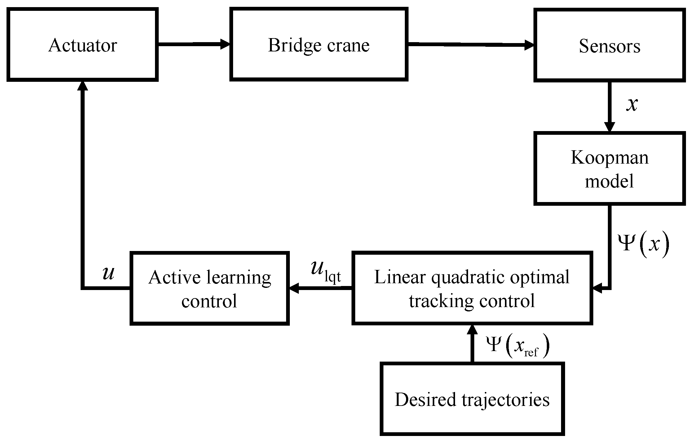
This section presents the controller framework, as shown in Figure 2. The proposed controller can achieve positioning and anti-swing control of the bridge crane, and the design of controller does not depend on the model of the system itself. Unlike other data-driven control methods, the proposed controller does not require the data-driven model to be trained in advance, and only requires real-time input and output data of the bridge crane system to accurately build the Koopman model by learning the Koopman operator.

3.1. Objective Function Design

The active learning controller allows the bridge crane to guide itself towards the important regions of the state space while tracking the trajectory, thereby improving data collection and the quality of the learned Koopman model. Therefore, we consider a general objective function of the form
J 1 = 0 l learn ( z ( t ) , u ( t ) ) + l task ( z ( t ) , u ( t ) ) d t + l final ( z ( T ) ) ,
where z ( t ) is the value of the function observables at time t subject to the Koopman model in (10), starting from initial condition z ( 0 ) = Ψ ( x ( 0 ) ) and with u ( t ) as the input at time t, T the prediction horizons, l task designed to accurately evaluate the proximity to the desired trajectory, l learn designed to evaluate the accuracy of the learned Koopman model, and l final the terminal cost.
In this work, we use the Fisher information [32] to generate an information measure in l learn . The Fisher information is a way of measuring how much information a random variable has with respect to a set of parameters. We can compute the Fisher information matrix F over the parameters that compose the approximate continuous-time operator G ˜ , with the elements in row a and column b of the Fisher information matrix being
F a , b = f z G ˜ a , b Σ 1 f z G ˜ a , b ,
where G ˜ a , b represents the elements in row a and column b of the approximate continuous-time operator G ˜ and Σ is the noise covariance matrix. Because the Fisher information F defined here is positive semi-definite, we use the trace of the Fisher information matrix F as the T-optimality measure J ( G ˜ ) [33]. Thus, the T-optimality measure is defined as
J ( G ˜ ) = tr ( F ) ,
where tr ( · ) represents the trace of the matrix.
Therefore, the learning cost l learn is defined as
l learn ( z ( t ) , u ( t ) ) = σ J ( G ˜ ) + ϵ ,
where ϵ 1 is a small number to prevent singular solutions due to the positive semi-definite Fisher information matrix, σ is the information weight, and J is computed using the evaluation of G ˜ at the current time.
Remark 1.
Typically, the information weight σ is time-varying and should be set to gradually decrease during the learning process [20]. For instance, we can set σ ( t ) = σ 0 ( 1 0.01 ) t , with σ 0 being an initial information weight.
At the same time, in order to match the desired trajectory, the running cost l task is defined as
l task ( z ( t ) , u ( t ) ) = z ( t ) z ref ( t ) Q ¯ + u ( t ) R ¯ ,
where Q ¯ represents the lifted state cost matrix provided by [ Q 0 ; 0 0 ] , with Q penalizing the system states and R ¯ the control cost matrix, z ref = Ψ ( x ref ) , and the desired trajectory of the Koopman model (10) obtained by lifting the desired trajectory of the original system (1) using observables Ψ .
The terminal cost is defined as
l final ( z ( T ) ) = z ( T ) Q f z ( T ) ,
where Q f represents terminal cost matrix and z ( T ) is the value of the function observables at time T subject to the Koopman model in (10) starting from initial condition z ( 0 ) .

3.2. Linear Quadratic Optimal Tracking

Next, we design a linear quadratic regulator (LQR) in the lifted states in order to track the reference trajectories using a linear predictor.
Consider the Koopman model (10). To track reference trajectories x ref , we design an LQT controller that minimizes a running cost (15) and terminal cost (16) in a receding-horizon fashion. At the current time, we lift the original state x ( 0 ) to find z ( 0 ) using the observables Ψ ( · ) ; the optimal control u lqt ( 0 ) can be obtained by solving the following optimization problem:
min u lqt 0 l task ( z ( t ) , u lqt ( t ) ) d t + l final ( z ( T ) )
subject to
(17b) z ˙ ( t ) = A z ( t ) + B u lqt ( t ) , (17c) z ( 0 ) = Ψ ( x ( 0 ) ) .
Because the running cost (15) is quadratic and the constraints are linear, the solution can be found by solving the algebraic Riccati equation.
The LQT controller takes the form
u lqt ( t ) = K ( t ) z ( t ) + s ( t ) ,
where K ( t ) = R ¯ 1 B P ( t ) , the matrix P ( t ) , and the tracking compensation term s ( t ) can be satisfied via backwards integration of the Riccati differential equation
P ˙ ( t ) = Q ¯ + P ( t ) B R ¯ 1 B P ( t ) P ( t ) A A P ( t ) ,
s ˙ ( t ) = A s + P ( t ) B R ¯ 1 B s ( t ) + Q ¯ z r e f ,
from the final conditions
P ( T ) = Q f ,
s ( T ) = Q f z ref ( T ) .

3.3. Active Learning Controller

When the amount of data obtained by the controller is small, there is a significant gap between the learned Koopman model and the infinite-dimensional Koopman operator model. Therefore, the LQT controller (18) designed based on the Koopman model cannot ensure that the trolley reaches the target position, and may even deviate far from the target position.
In light of Equation (11), we want to synthesize a controller that can ensure that the trolley reaches the target position while allowing for improvements in the information measure used for active learning. To achieve this, we design an active learning controller by minimizing the objective function J 1 (11) based on the LQT controller. For this, we need to know how sensitive the objective function J 1 (11) is to switching between the LQT control u lqt and the active learning control u al at time τ for a time duration λ .
The sensitivity of switching from u lqt to u al for all τ [ 0 , T ] for an infinitesimally small λ (known as the mode insertion gradient [34]) is provided by
J 1 λ | τ , λ = 0 = ρ ( τ ) ( f 2 f 1 ) ,
where z ( t ) is a solution to the Koopman model (10) under control u ( t ) = u lqt ( t ) (18), f 1 = f z ( z ( τ ) , u lqt ( τ ) ) , f 2 = f z ( z ( τ ) , u al ( τ ) ) , and
ρ ˙ ( t ) = l learn z l task z u lqt z ( l learn u + l task u ) ( f z z + f z u u lqt z ) ρ ( t )
subject to the terminal condition ρ ( T ) = 0 .
By minimizing the mode insertion gradient within the predicted time period t [ 0 , T ] , we are able to obtain the desired active learning controller u al ( t ) . Therefore, we can write an unconstrained optimization problem using a secondary objective function
J 2 = 0 J 1 λ | τ = t , λ = 0 + 1 2 u al ( t ) u lqt ( t ) R ^ 2 d t ,
where R ^ R m × m bounds the gap between u al ( t ) and u lqt ( t ) and where J 1 λ | τ = t , λ = 0 is evaluated at τ = t .
Proposition 1.
The active learning controller u al ( t ) that minimizes (23) is
u al ( t ) = R ^ 1 B ρ ( t ) + u lqt ( t ) .
Proof. 
Because (23) is separable in time, we take the derivative of (23) with respect to u al ( t ) at each point in t, which provides the following expression:
u al J 2 = 0 T u al ( ρ ( τ ) ( f 2 f 1 ) + 1 2 ( u al ( t ) u lqt ( t ) ) R ^ ( u al ( t ) u lqt ( t ) ) ) d t = 0 T B ρ ( t ) + R ^ ( u al ( t ) u lqt ( t ) ) d t .
The resulting equation can be obtained as follows:
0 T B ρ ( t ) + R ^ ( u al ( t ) u lqt ( t ) ) d t = 0 .
Finally, solving for u al ( t ) in (25) results in the solution
u al ( t ) = R ^ 1 B ρ ( t ) + u lqt ( t ) .
The active learning control u al ( t ) at time t = 0 is taken as the actual control acting on the controlled system (1) at the current moment. The approximate continuous-time operator G ˜ is updated by obtaining the real-time input and output states of the bridge crane. The Koopman model (3) is reconstructed using the updated continuous-time operator in the next control cycle for optimization and finding a solution. The above process is repeated to complete rolling optimization within the control time domain and realize active learning control for the bridge crane.
Remark 2.
The system parameters of the bridge crane system may change; for instance, there may be changes in the friction coefficient caused by the weather or other factors, changes in load quality, changes in rope length, etc. Traditional data-driven algorithms are based on offline data used to train models in advance. When the parameters change, these trained models may no longer be a good match, resulting in unsatisfactory control performance. On the other hand, the active learning approach is based on online data, which continues to be applicable even when the system parameters change.
The steps in the proposed active learning control methodology are as follows.
Step 1.
Define a set of observable functions; given an initial approximate continuous-time operator, construct the Koopman model.
Step 2.
Pre-set the desired trajectory and lift it using the observable function.
Step 3.
Design the linear quadratic optimal tracking controller based on the Koopman model and the desired trajectory.
Step 4.
Consider both the learning and running costs, design an active learning controller based on the linear quadratic optimal tracking controller.
Step 5.
Apply the active learning controller to the bridge crane at the current time and obtain the output after the control is applied.
Step 6.
Update the approximate continuous-time operator using the online input and output data.
Step 7.
Reconstruct the Koopman model using the updated continuous-time operator and repeat Steps 3–7.

4. Simulation

In order to verify the effectiveness of the proposed active learning method, simulations were conducted in the Python environment. According to the motion characteristics of the bridge crane, the constraints for the system during the simulation tests were as follows: the horizontal displacement constraint of trolley was [ 0 , 2 ] m ; the velocity constraint of the trolley was [ 5 , 5 ] m / s ; the swing angle constraint of the load was [ 90 , 90 ] deg ; and the control input constraint was [ 25 , 25 ] N . The physical parameters of the bridge crane and the parameters of the active learning controller are provided in Table 1. We denote ξ : = [ y , θ , y ˙ , θ ˙ , sin ( y ) , sin ( θ ) , sin ( y ˙ ) , sin ( θ ˙ ) , cos ( y ) , cos ( θ ) , cos ( y ˙ ) , cos ( θ ˙ ) ] R 12 , and the observable in the lifted space is chosen as Ψ ( x ) = [ ξ 1 , , ξ 12 , ξ 1 ξ 2 , , ξ 11 ξ 12 ] R 78 .

4.1. Performance Evaluation for Active Learning Controller without Training in Advance

To assess the effectiveness of the proposed method, the active learning controller was applied to the bridge crane system (1) for the first time without training in advance. Instead of obtaining historical data to train the Koopman model in advance, we used random initialization. Considering a control without any nonlinear characteristic, we ran the simulation for t = 60 s with a sampling rate of t s , as shown in Figure 3.
At first, the desired position of the trolley was set as y ref = 0.50 m . Due to the lack of prior training, in the first 15 s the controller needs to learn the Koopman operator in order to establish the Koopman model. Therefore, the trolley does not immediately reach the desired position, and the load swing angle is large. After the controller learns the Koopman operator and establishes the model, the trolley immediately moves to the desired position of 0.5 m while ensuring that there is no load swing. At t = 40 s, the desired position of the trolley is set as y ref = 1.50 m . Due to the controller having learned an accurate Koopman model, the trolley quickly reaches the desired position and the load swing remain small.

4.2. Comparative Study

For the purpose of better verifying the performance of the proposed method, two other control methods, namely, conventional sliding mode control (CSMC) [1] and PID [35], were selected to compare the control effect on the bridge crane system. The expressions of the two controllers used for comparison are provided below.

4.2.1. CSMC Controller

u ( t ) = ( M + m sin ( θ ( t ) ) 2 ) [ K s p ( t ) η sgn ( s p ( t ) ) c 1 y ˙ ( t ) c 2 θ ˙ ( t ) + μ y ˙ ( t ) m g sin ( θ ( t ) ) cos ( θ ( t ) ) m l θ ( t ) ˙ 2 sin ( θ ( t ) ) M + m sin ( θ ( t ) ) 2 + g sin ( θ ( t ) ) l ]
where c 1 , c 2 , c 3 denote the sliding constants, η , K represents the gain of sliding mode surface, and s p is the position of the sliding mode surface, which is defined as follows:
s p ( t ) = y ˙ ( t ) + c 1 ( y ( t ) y ref ( t ) ) + c 2 θ ( t )
where y ref is the desired horizontal displacement trajectory of y.

4.2.2. PID Controller

u ( t ) = k y p ( y ( t ) y ref ( t ) ) + k y i 0 t ( y ( τ ) y ref ( τ ) ) d τ + k 1 d y ˙ ( t ) + k θ p θ ( t ) + k θ i 0 t θ ( τ ) d τ + k θ d θ ˙ ( t ) ,
where k y p , k y i , k y d , k θ p , k θ i , k θ d represent the control gains.
The parameters of the CSMC controller and PID controller used in the experiments are provided in Table 2. Figure 4 presents the performance curves of all three controllers. It can be seen that the CSMC controller requires less crane operating positioning time and has payload swing compared to the PID controller. With our active learning control, the system can reach the desired position quickly with tolerable oscillations, while with CSMC the system reaches the desired position somewhat slower and with more limited oscillations. Note that CSMC is a model-based controller designed based on the model’s knowledge, which means that the design of the CSMC controller requires a known system model and accurate parameters. On the other hand, our approach uses a data-driven approach. The active learning control can achieve similar control effects when the system model is unknown; in this case, the absence of accurate system parameters means that the system has better robustness when using the proposed approach.

4.3. Robustness Study

To further validate the robustness of the bridge crane system when using the proposed approach, the following three groups of simulation experiments were set up based on different working conditions, such as the payload, rope length, and friction coefficient changes in engineering applications.

4.3.1. Simulation Group 1

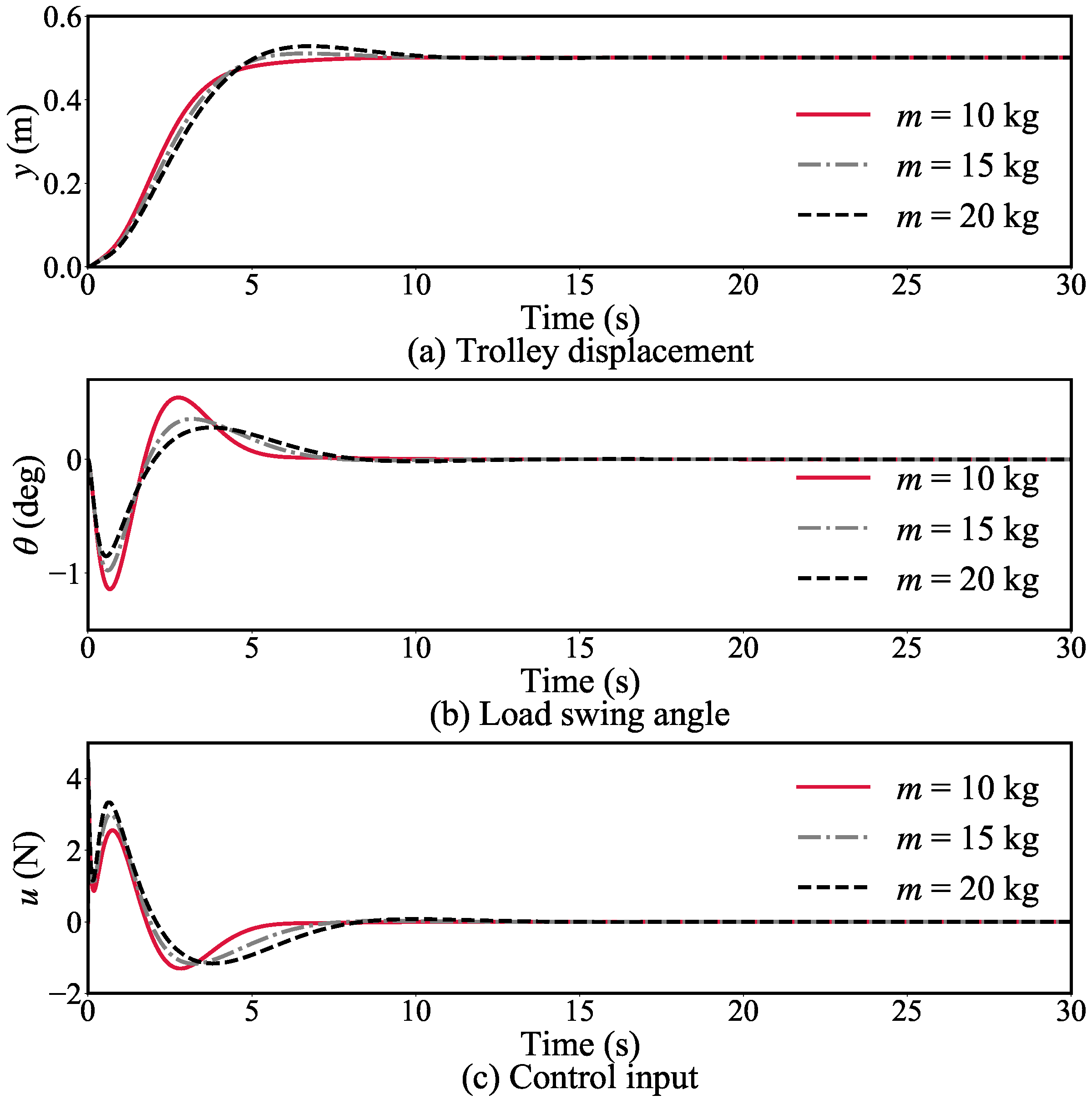
Simulation experiments were conducted with the system parameter settings in Table 1 remaining the same except for the payload mass. In these experiments, the mass of the payload m was selected as 10 kg, 15 kg, and 20 kg.
Figure 5 refers to the variation curves of various state quantities of the bridge crane system with the active learning controller under different payload mass conditions.

4.3.2. Simulation Group 2

To assess the influence of changes in the rope length on the bridge crane system, the rope length was changed while keeping the other controller parameters consistent. The rope length l was selected as 1.0 m, 1.5 m, and 2.0 m. The simulation results are shown in Figure 6.
It is shown that when the rope length changes while keeping the controller parameters unchanged, the proposed method achieves better positioning control and a relatively small maximum load swing angle.

4.3.3. Simulation Group 3

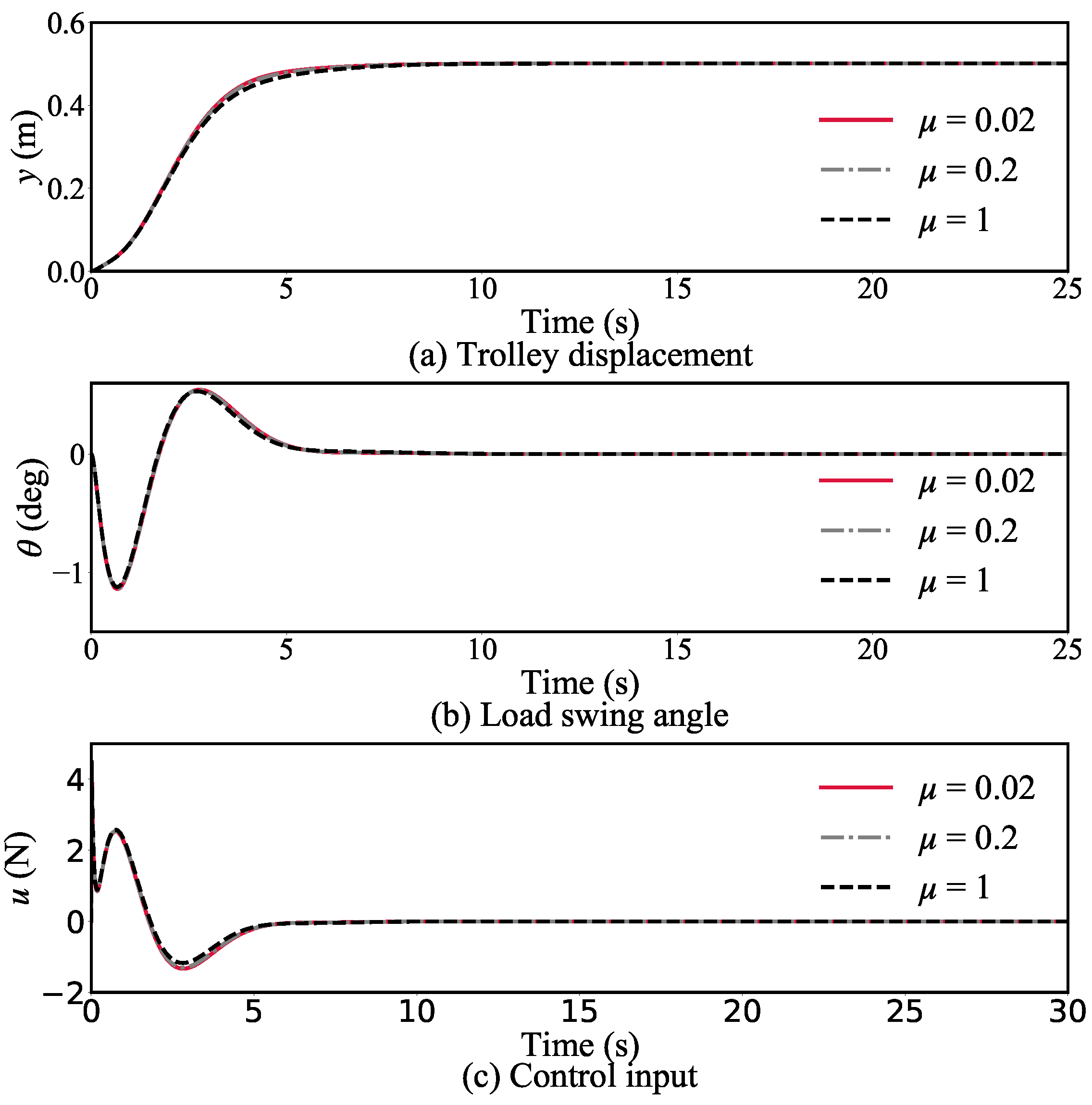
This group describes the changes in the control effect in the whole process with the active learning controller and under different track friction conditions. The other system parameter settings remained the same, while the friction coefficient between the crane and the track was adopted as μ = 0.02 , 0.2 , and 1. The results are shown in Figure 7.
With a changing friction coefficient, the sensitivity of the system is even lower. From Figure 7a,b, it can be seen that the control performance curves of the system under the three friction coefficients are essentially superimposed on one another.
In summary, these three simulation experiments verify that the active learning controller is less sensitive than others to changes in model parameters, specifically, the load mass, rope length, and friction coefficient, and that the proposed system has strong robustness.

4.4. Performance with Dead Zone

Due to the location of the transmission device between the gear and the track, a dead zone characteristic may exist in the bridge crane system. Therefore, in this subsection we consider the controller in a scenario with a dead zone, as follows:
u = u r r u r > r 0 r u r r u r + r u r < r
where u r ( t ) = u al ( t ) represents the control input calculated by the active learning controller and r is the dead zone parameter, which reflects the level of the dead zone.
Simulation experiments were conducted with the same system parameter settings provided in Table 1. We performed numerical simulations to assess the capability of the proposed active learning control in a scenario with the dead zone characteristic under different dead zone parameters. The dead zone parameter r was selected as 0.1 , 0.5 , 1, and 2. The desired position of trolley was set as y ref = 0.5 m. Figure 8 presents the simulation results of the bridge crane system with the active learning controller and input dead zone parameters. Figure 8a,b shows that when r = 0.1 , i.e., the dead zone characteristic is not significant, the bridge crane system can quickly reach the desired position with a steady-state error of only 0.008 m and with only smooth and minor swinging of the rope. As the value of the dead zone parameter r increases, the steady-state error between the real position and the desired position gradually increases and the swinging of the rope grows more prominent. Due to the existence of the dead zone characteristic, the nonlinear controller u in (30) is applied to the system instead of the desired active learning control input u r shown in Figure 8c. Therefore, the larger the dead zone parameter, the worse the control effect becomes.

5. Conclusions

In this paper, we have proposed an active learning control for bridge cranes without the need for training in advance. In the proposed approach, the Koopman operator is used to enhance the control effect of the bridge crane system. Using only the real-time online input and output data of the bridge crane system, the active learning control method consists of finite-dimensional approximation of Koopman operator and the design of an active learning controller based on linear quadratic optimal tracking control. The effectiveness of this method has been verified through numerical simulations. The proposed control method has a simple structure, good tracking performance, and strong robustness for bridge cranes.

Author Contributions

Conceptualization, H.L. and X.L.; methodology, H.L. and X.L.; validation, H.L. and X.L.; formal analysis, H.L.; software, H.L.; writing—original draft preparation, H.L.; writing—review and editing, H.L. and X.L.; supervision, X.L. All authors have read and agreed to the published version of the manuscript.

Funding

This research received no external funding.

Acknowledgments

The authors would like to thank the anonymous referees for their constructive comments and express their gratitude to Qian Ye for her valuable inputs.

Conflicts of Interest

The authors declare no conflict of interest.

References

  1. Wang, T.L.; Tan, N.L.; Zhang, X.; Li, G.; Su, S.; Zhou, J.; Qiu, J.; Wu, Z.; Zhai, Y.; Donida, L.R.; et al. A Time-Varying Sliding Mode Control Method for Distributed-Mass Double Pendulum Bridge Crane With Variable Parameters. IEEE Access 2021, 9, 75981–75992. [Google Scholar] [CrossRef]
  2. Tysse, G.O.; Cibicik, A.; Tingelstad, L.; Egeland, O. Lyapunov-based damping controller with nonlinear MPC control of payload position for a knuckle boom crane. Automatica 2022, 140, 110219. [Google Scholar] [CrossRef]
  3. Roman, R.C.; Precup, R.E.; Petriu, E.M. Hybrid data-driven fuzzy active disturbance rejection control for tower crane systems. Eur. J. Control 2021, 58, 373–387. [Google Scholar] [CrossRef]
  4. Rigatos, G.; Siano, P.; Abbaszadeh, M. Nonlinear H-infinity control for 4-DOF underactuated overhead cranes. Trans. Inst. Meas. Control 2018, 40, 2364–2377. [Google Scholar] [CrossRef]
  5. Hou, Z.S.; Bu, X.H. Model free adaptive control with data dropouts. Expert Syst. Appl. 2011, 38, 10709–10717. [Google Scholar] [CrossRef]
  6. Furqan, M.; Cheng, S. Data-driven optimal PID type ILC for a class of nonlinear batch process. Int. J. Syst. Sci. 2021, 52, 263–276. [Google Scholar] [CrossRef]
  7. Chi, R.H.; Li, H.Y.; Shen, D.; Hou, Z.S.; Huang, B. Enhanced P-Type Control: Indirect Adaptive Learning From Set-Point Updates. IEEE Trans. Autom. Control 2023, 68, 1600–1613. [Google Scholar] [CrossRef]
  8. Estakhrouiyeh, M.R.; Gharaveisi, A.; Vali, M. Fractional order Proportional-Integral-Derivative Controller parameter selection based on iterative feedback tuning. Case study: Ball Levitation system. Trans. Inst. Meas. Control 2018, 40, 1776–1787. [Google Scholar] [CrossRef]
  9. Yuan, Y.; Tang, L.X. Novel time-space network flow formulation and approximate dynamic programming approach for the crane scheduling in a coil warehouse. Eur. J. Oper. Res. 2017, 262, 424–437. [Google Scholar] [CrossRef]
  10. Williams, M.O.; Hemati, M.S.; Dawson, S.T.M.; Kevrekidis, I.G.; Rowley, C.W. Extending Data-Driven Koopman Analysis to Actuated Systems. IFAC-PapersOnLine 2016, 49, 704–709. [Google Scholar] [CrossRef]
  11. Proctor, J.L.; Brunton, S.L.; Kutz, J.N. Generalizing Koopman Theory to Allow for Inputs and Control. SIAM J. Appl. Dyn. Syst. 2018, 17, 909–930. [Google Scholar] [CrossRef] [PubMed]
  12. Maksakov, A.; Golovin, I.; Shysh, M.; Palis, S. Data-driven modeling for damping and positioning control of gantry crane. Mech. Syst. Signal. Pract. 2023, 197, 110368. [Google Scholar] [CrossRef]
  13. Brunton, S.L.; Brunton, B.W.; Proctor, J.L.; Kutz, J.N. Koopman Invariant Subspaces and Finite Linear Representations of Nonlinear Dynamical Systems for Control. PLoS ONE 2016, 2, e0150171. [Google Scholar] [CrossRef] [PubMed]
  14. Schmid, P.J. Dynamic mode decomposition of numerical and experimental data. J. Fluid Mech. 2010, 656, 5–28. [Google Scholar] [CrossRef]
  15. Williams, M.O.; Kevrekidis, I.G.; Rowley, C.W. A data–driven approximation of the Koopman operator: Extending dynamic mode decomposition. J. Nonlinear Sci. 2015, 25, 1307–1346. [Google Scholar] [CrossRef]
  16. Kaiser, E.; Kutz, J.N.; Brunton, S.L. Data-driven discovery of Koopman eigenfunctions for control. Mach. Learn. Sci. Technol. 2021, 2, 035023. [Google Scholar] [CrossRef]
  17. Maksakov, A.; Golovin, I.; Palis, S. Koopman–based data-driven control for large gantry cranes. In Proceedings of the 2022 IEEE 3rd KhPI Week on Advanced Technology (KhPIWeek), Kharkiv, Ukraine, 3–7 October 2022; pp. 1–5. [Google Scholar] [CrossRef]
  18. Baranes, A.; Oudeyer, P.Y. Active learning of inverse models with intrinsically motivated goal exploration in robots. Robot. Auton. Syst. 2013, 61, 49–73. [Google Scholar] [CrossRef]
  19. Kober, J.; Bagnell, J.A.; Peter, J. Reinforcement learning in robotics: A survey. Int. J. Robot. Res. 2013, 32, 1238–1274. [Google Scholar] [CrossRef]
  20. Abraham, I.; Murphey, T.D. Active Learning of Dynamics for Data-Driven Control Using Koopman Operators. IEEE Trans. Robot. 2019, 35, 1071–1083. [Google Scholar] [CrossRef]
  21. Wilson, A.D.; Schultz, J.A.; Ansari, A.R.; Murphey, T.D. Dynamic task execution using active parameter identification with the Baxter research robot. IEEE Trans. Autom. Sci. Eng. 2017, 14, 391–397. [Google Scholar] [CrossRef]
  22. Wilson, A.D.; Schultz, J.A.; Murphey, T.D. Trajectory synthesis for Fisher information maximization. IEEE Trans. Robot. 2014, 30, 1358–1370. [Google Scholar] [CrossRef] [PubMed]
  23. Mnih, V.; Badia, A.P.; Mirza, M.; Graves, A.; Lillicrap, T.; Tim, H.; Silver, D.; Kavukcuoglu, K. Asynchronous methods for deep reinforcement learning. In Proceedings of the 33rd International Conference on Machine Learning (PMLR), New York, NY, USA, 20–22 June 2016; pp. 1928–1937. [Google Scholar]
  24. Cutler, M.; Walsh, T.J.; How, J.P. Real–World Reinforcement Learning via Multifidelity Simulators. IEEE Trans. Robot. 2015, 31, 655–671. [Google Scholar] [CrossRef]
  25. Ding, F.; Wang, X.H.; Chen, Q.J.; Xiao, Y. Recursive Least Squares Parameter Estimation for a Class of Output Nonlinear Systems Based on the Model Decomposition. Circuits Syst. Signal Process. 2016, 35, 3323–3338. [Google Scholar] [CrossRef]
  26. Williams, G.; Wagener, N.; Goldfain, B.; Drews, P.; Rehg, J.M.; Boots, B.; Theodorou, E.A. Information theoretic MPC for model-based reinforcement learning. In Proceedings of the 2017 IEEE International Conference on Robotics and Automation (ICRA), Singapore, 29 May–3 June 2017; pp. 1714–1721. [Google Scholar] [CrossRef]
  27. Bonnet, V.; Fraisse, P.; Crosnier, A.; Gautier, M.; González, A.; Venture, G. Optimal exciting dance for identifying inertial parameters of an anthropomorphic structure. IEEE Trans. Robot. 2016, 32, 823–836. [Google Scholar] [CrossRef]
  28. Jovic, J.; Escande, A.; Ayusawa, K.; Yoshida, E.; Kheddar, A.; Venture, G. Humanoid and human inertia parameter identification using hierarchical optimization. IEEE Trans. Robot. 2016, 32, 726–735. [Google Scholar] [CrossRef]
  29. Korda, M.; Mezić, I. Linear predictors for nonlinear dynamical systems: Koopman operator meets model predictive control. Automatica 2018, 93, 149–160. [Google Scholar] [CrossRef]
  30. Arbabi, H.; Korda, M.; Mezić, I. A Data-Driven Koopman Model Predictive Control Framework for Nonlinear Partial Differential Equations. In Proceedings of the 2018 IEEE Conference on Decision and Control (CDC), Miami, FL, USA, 7–19 December 2018; pp. 6409–6414. [Google Scholar] [CrossRef]
  31. Antsaklis, P.J.; Michel, A.N. A Linear System; Springer: New York, NY, USA, 2006. [Google Scholar]
  32. Pukelsheim, F. Optimal Design of Experiments; SIAM: Philadelphia, PA, USA, 2006. [Google Scholar]
  33. Nahi, N.E.; Napjus, G.A. Design of optimal probing signals for vector parameter estimation. In Proceedings of the 1971 IEEE Conference on Decision and Control (CDC), Miami Beach, FL, USA, 15–17 December 1971; pp. 162–168. [Google Scholar] [CrossRef]
  34. Egerstedt, M.; Wardi, Y.; Delmotte, F. Optimal control of switching times in switched dynamical systems. In Proceedings of the 42nd IEEE International Conference on Decision and Control (IEEE Cat. No.03CH37475), Maui, HI, USA, 9–12 December 2003; pp. 2138–2143. [Google Scholar] [CrossRef]
  35. Sun, Z.; Ling, Y.; Tang, X.; Zhou, Y.; Sun, Z.X. Designing and application of type-2 fuzzy PID control for overhead crane systems. Int. J. Intell. Robot. 2021, 5, 10–22. [Google Scholar] [CrossRef]
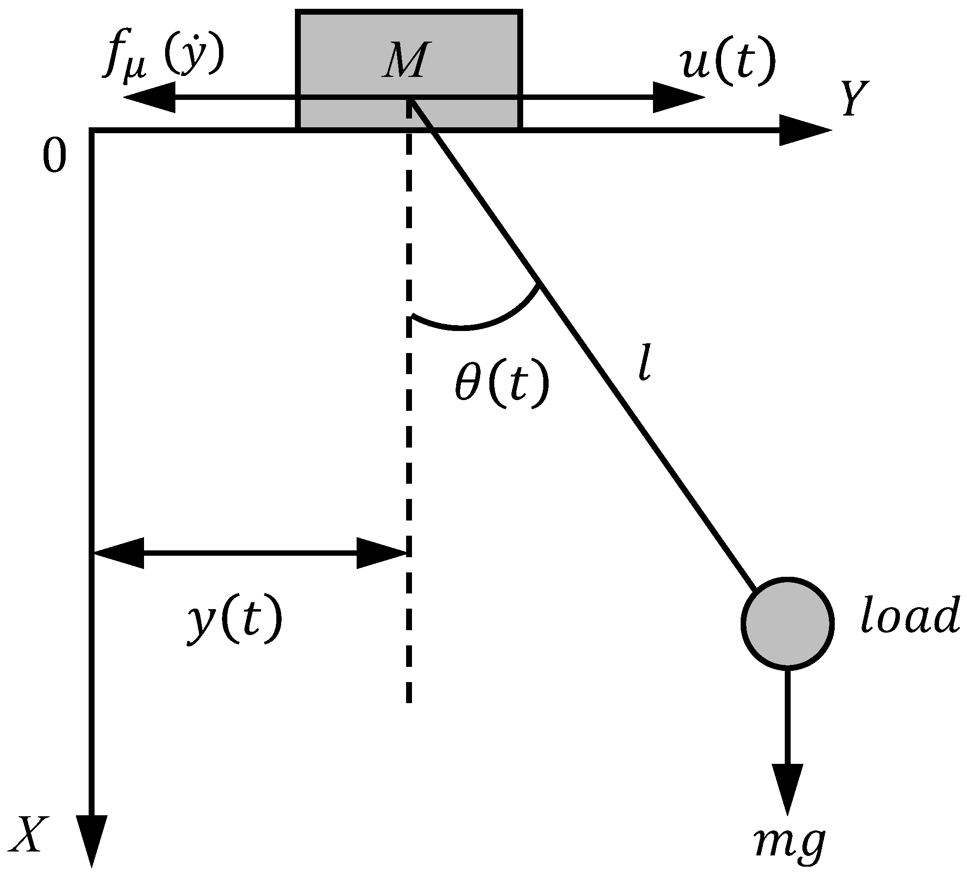
Figure 1. 2D model of bridge crane.
Mca 28 00101 g001
Figure 2. Control block diagram.
Mca 28 00101 g002
Figure 3. Simulation results without training in advance.
Mca 28 00101 g003
Figure 4. Results of the comparative experiment using three different control methods.
Mca 28 00101 g004
Figure 5. Simulation results with different payload masses.
Mca 28 00101 g005
Figure 6. Simulation results with different lengths of hoisting rope.
Mca 28 00101 g006
Figure 7. Simulation results with different friction coefficients.
Mca 28 00101 g007
Figure 8. Simulation results with different dead zone parameters.
Mca 28 00101 g008
Table 1. The parameters of the bridge crane and active learning controller.
ParametersValue
Mass of trolley M ( kg ) 5
Mass of load m ( kg ) 10
Gravitational acceleration g ( m / s 2 ) 9.8
Length of hoisting rope l ( m ) 1
Friction coefficient μ 0.2
Predicted horizons T ( s ) 0.1
Sampling interval t s ( s ) 0.01
Dimension of the Koopman model L78
State penalty weight matrix Q 12000 0 0 0 0 1200 0 0 0 0 3000 0 0 0 0 500
Control weight matrix R ¯ 1
Initial information weight σ 200
Regularization weight R ^ 100
Terminal cost Q f 0
Table 2. Parameters of the CSMC and PID controllers.
ControllerParametersValue
CSMC controller c 1 0.3
c 2 10
η 0.001
K10
PID controller k y p 4
k y i 0.001
k y d 25
k θ p −0.1
k θ i 0.1
k θ d −1
Disclaimer/Publisher’s Note: The statements, opinions and data contained in all publications are solely those of the individual author(s) and contributor(s) and not of MDPI and/or the editor(s). MDPI and/or the editor(s) disclaim responsibility for any injury to people or property resulting from any ideas, methods, instructions or products referred to in the content.