
Enhanced MPPT-Based Fractional-Order PID for PV Systems Using Aquila Optimizer
 , ,
, ,  and
and 
Abstract
:1. Introduction
2. PV System Modeling
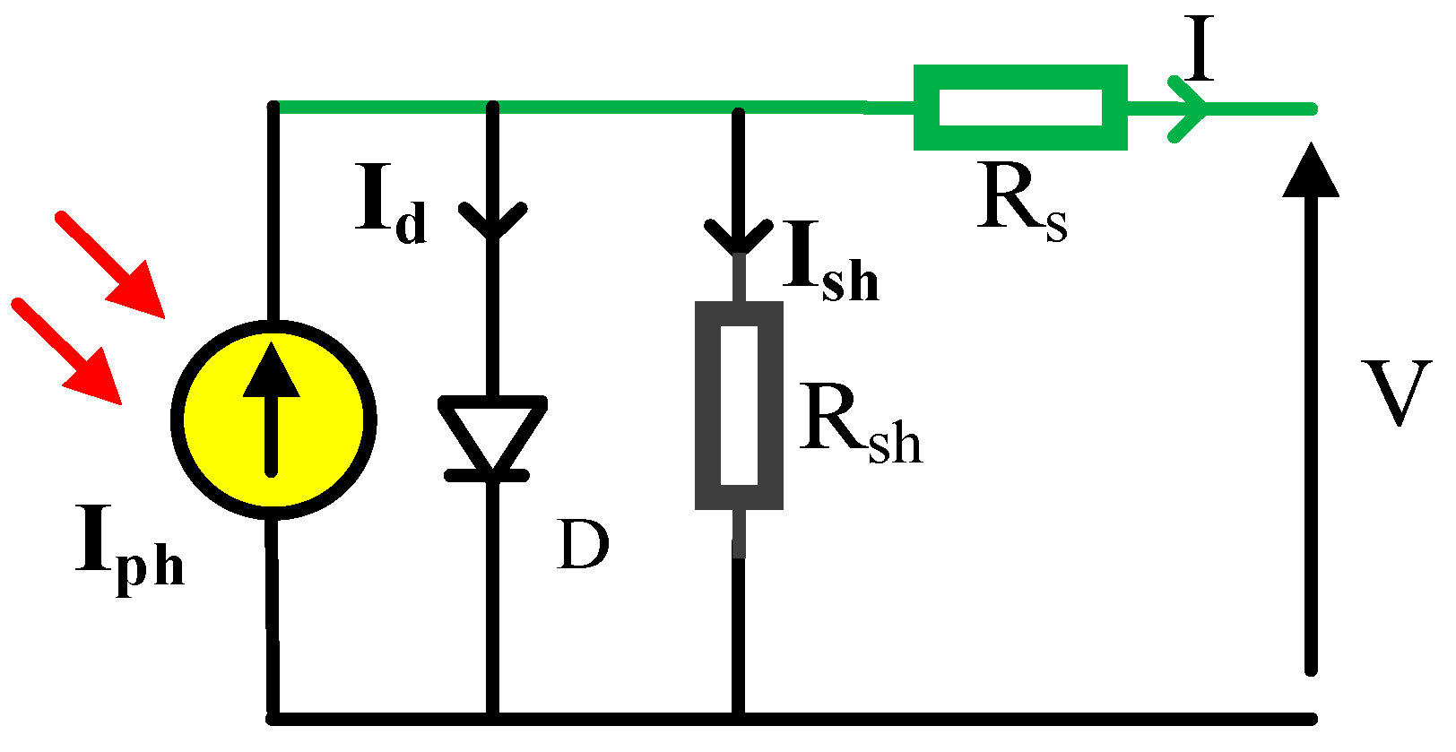
2.1. Modeling of PV Panel Single Diode Model
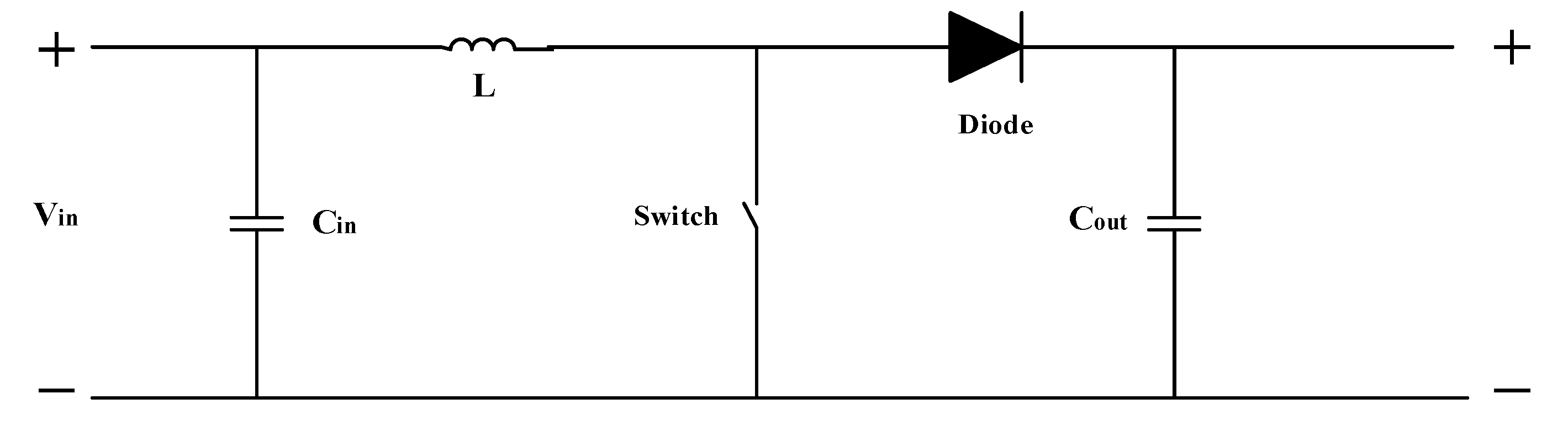
2.2. DC/DC Converter
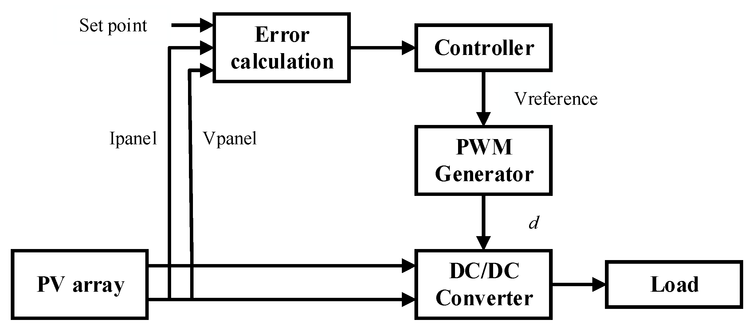
3. MPPT Control
3.1. MPPT dp/dv Feedback Method-Based Controller
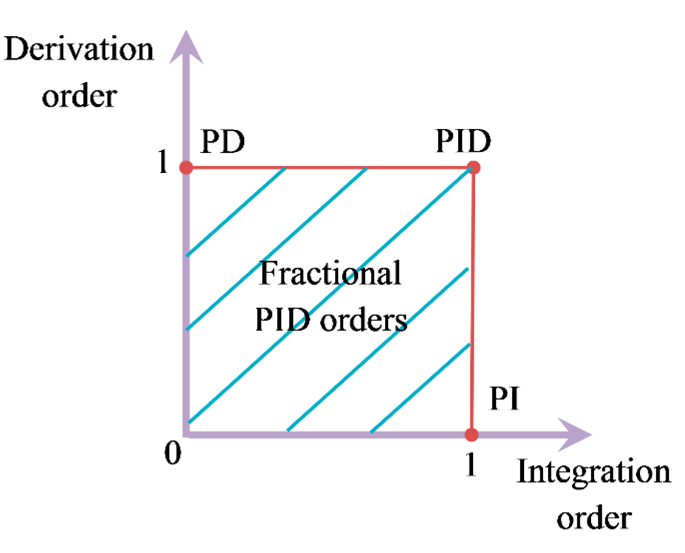
3.2. Fractional Calculus
3.3. PID Controller Description
3.4. Proposed Fractional-Order PID Controller
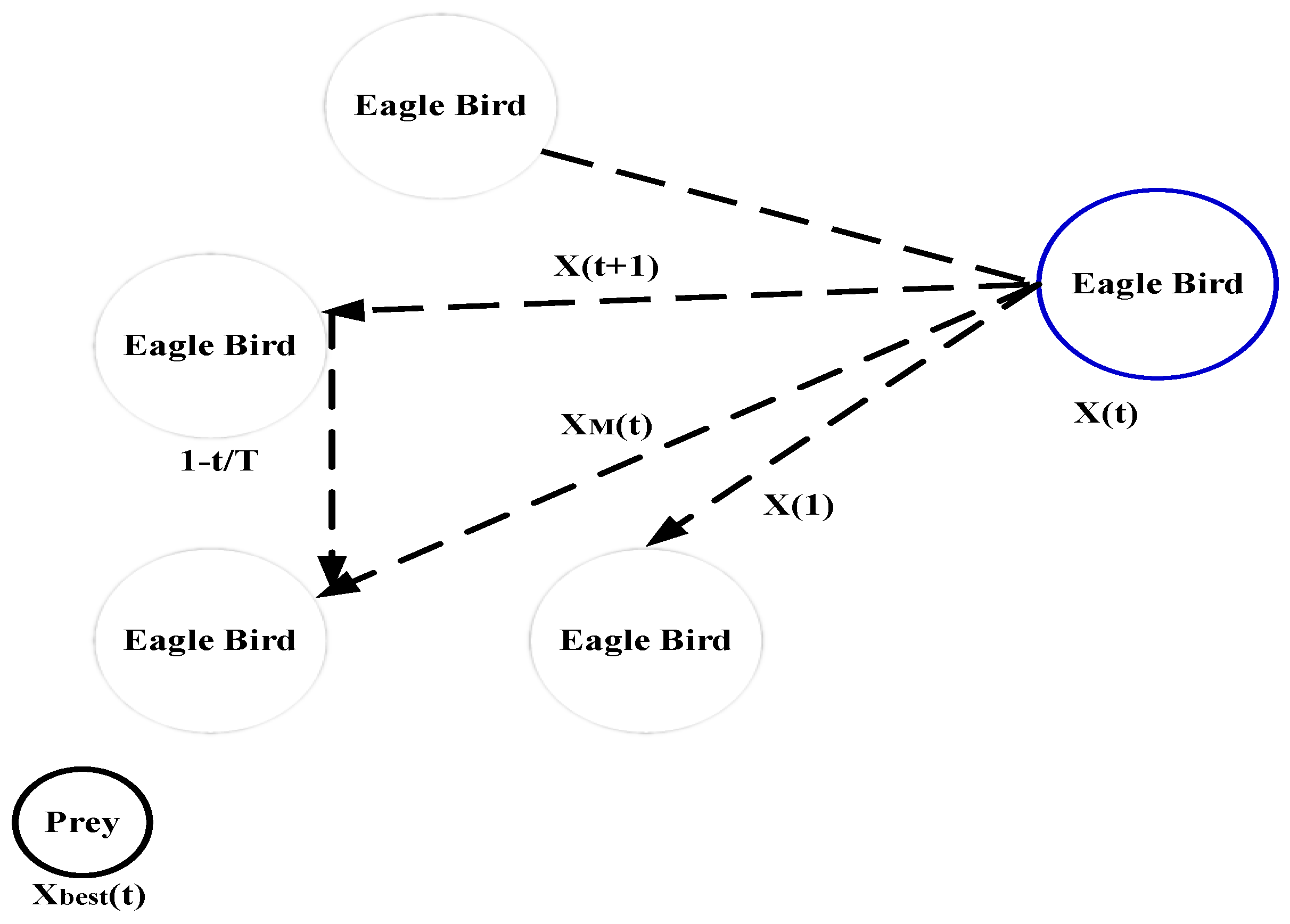
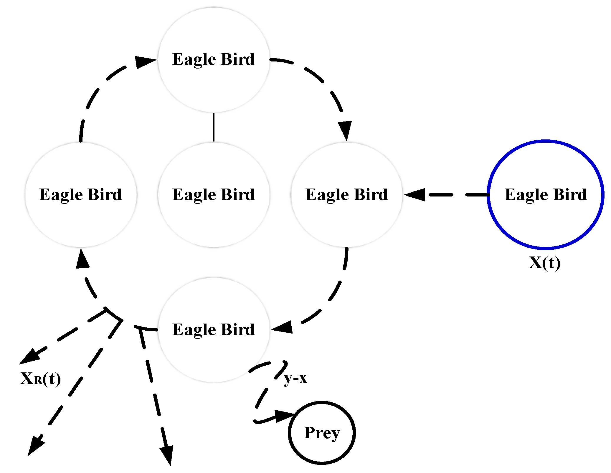
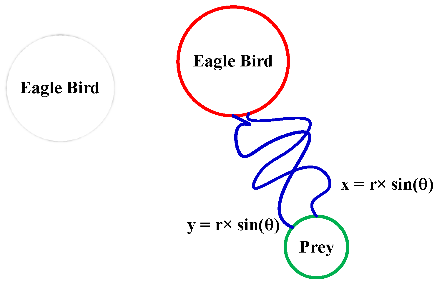
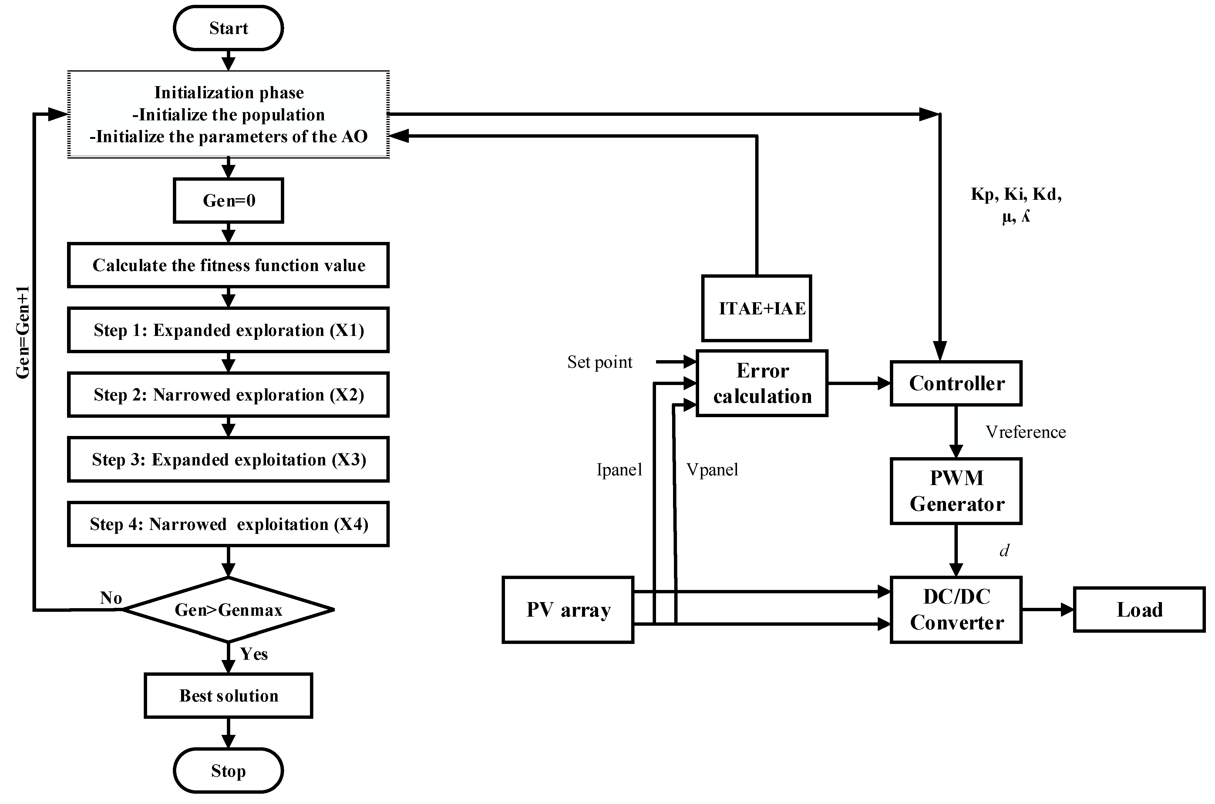
4. Aquila Optimizer
- Choosing the search boundary by elevated soaring and perpendicular stoop.
- Exploring within a diverged search boundary by a contour flight with a low glide swoop.
- Exploiting within a converged search boundary by a short flight with a slow drop swoop and swooping by walking and snatching the target.
4.1. Solution Initialization
4.2. Mathematical Formulation of AO
- Step 1: Expanded Exploration
- Step 2: Narrowed Exploration
- Step 3: Expanded Exploitation
- Step 4: Narrowed Exploitation
5. Fitness Function Formulation
6. Simulation Results and Discussion
6.1. MPPT Controller Performance Tests
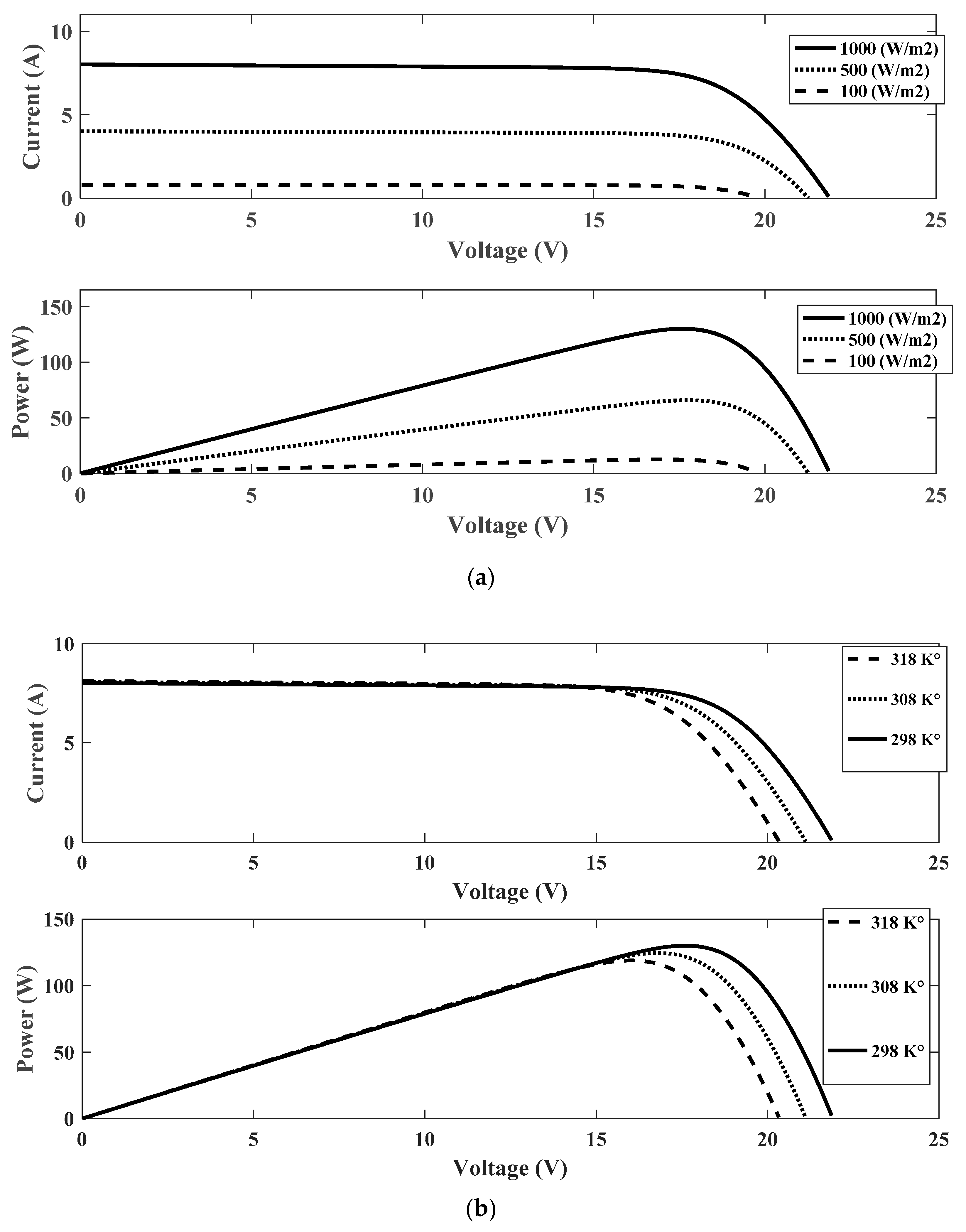
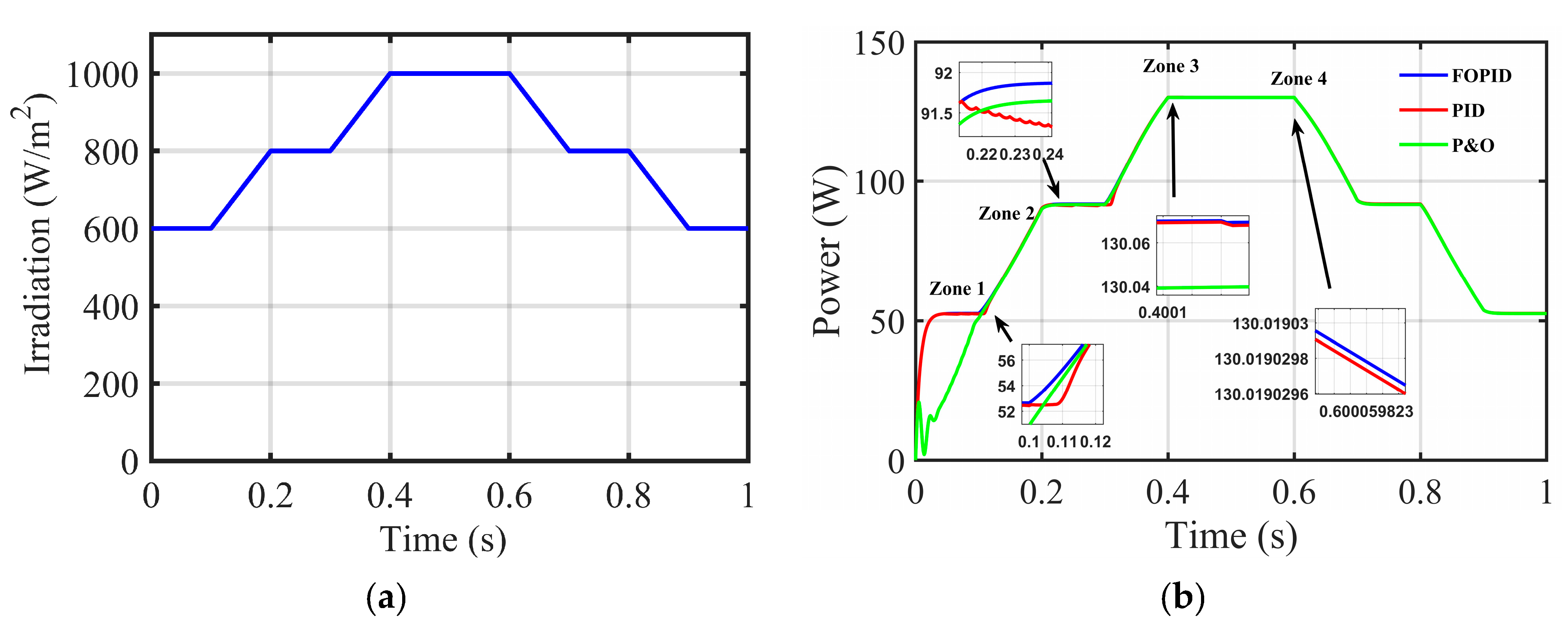
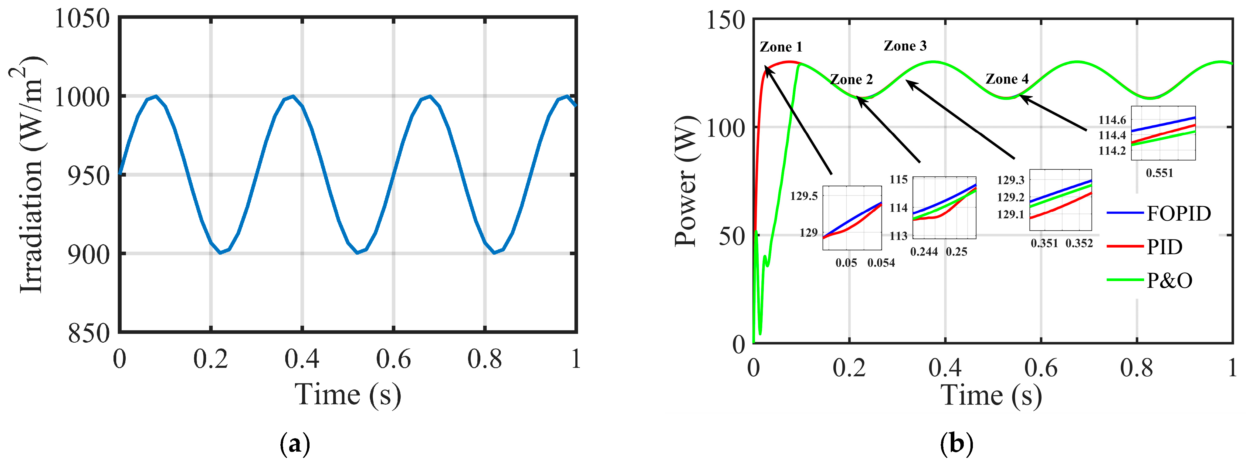
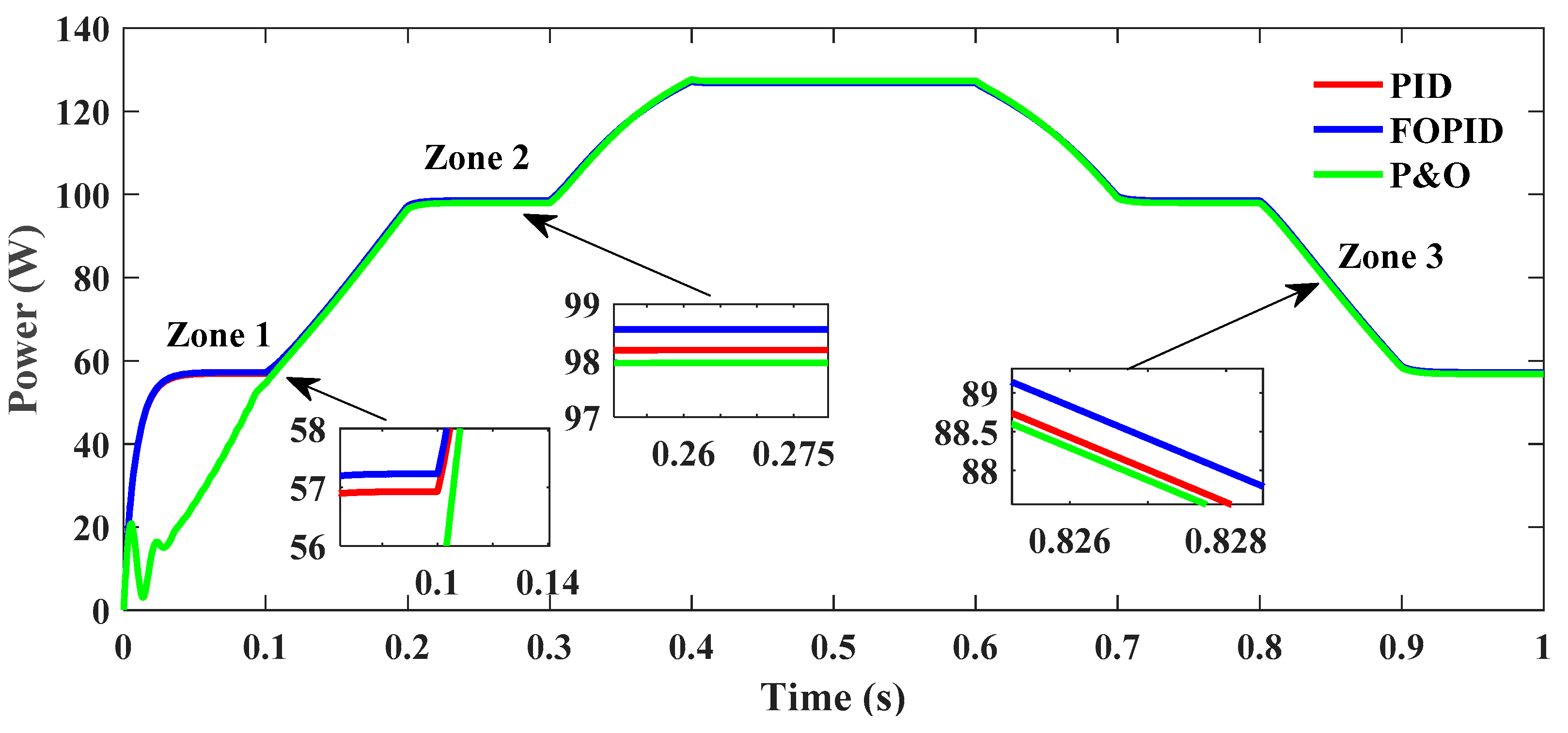
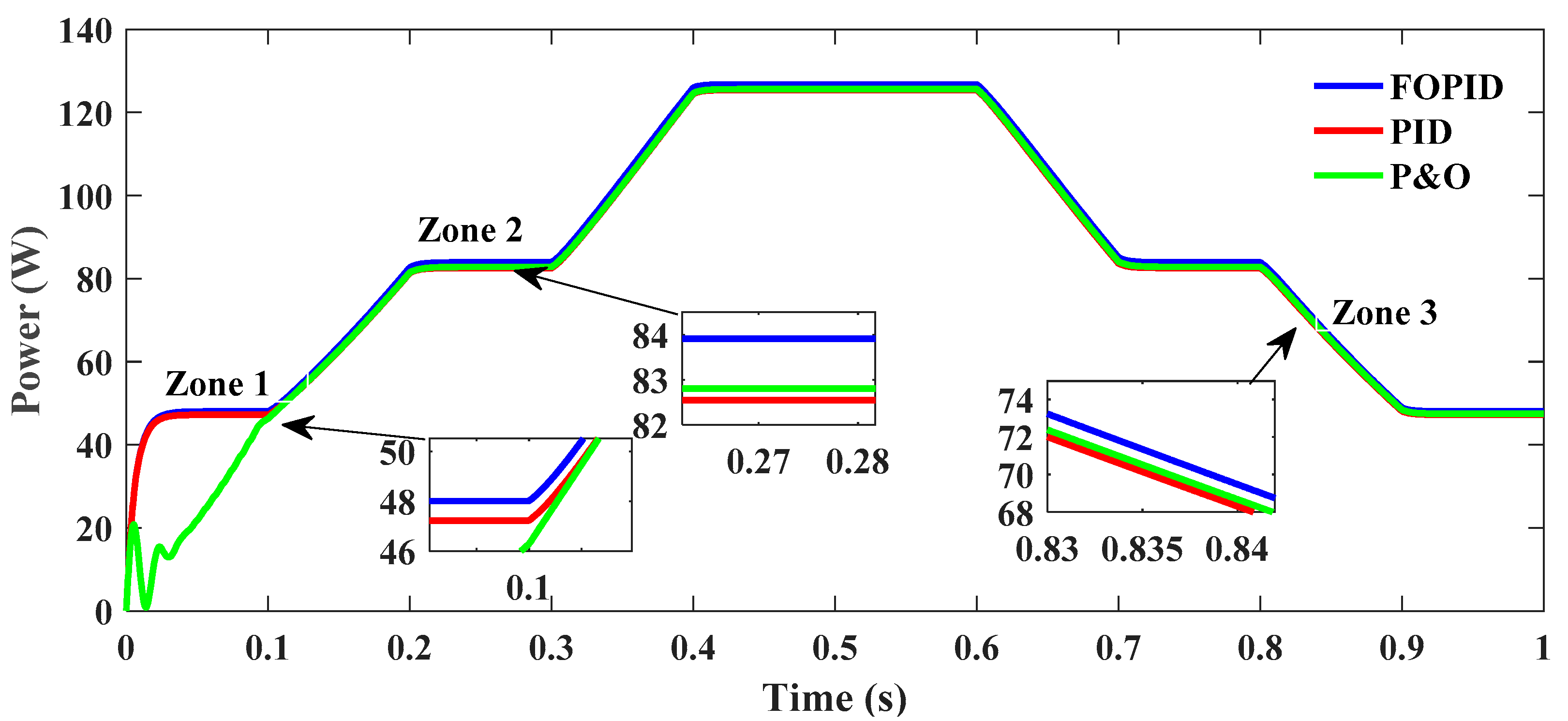
6.1.1. Irradiation Variation for Daytime Profile
6.1.2. Irradiation Variation for Sinusoidal Profile
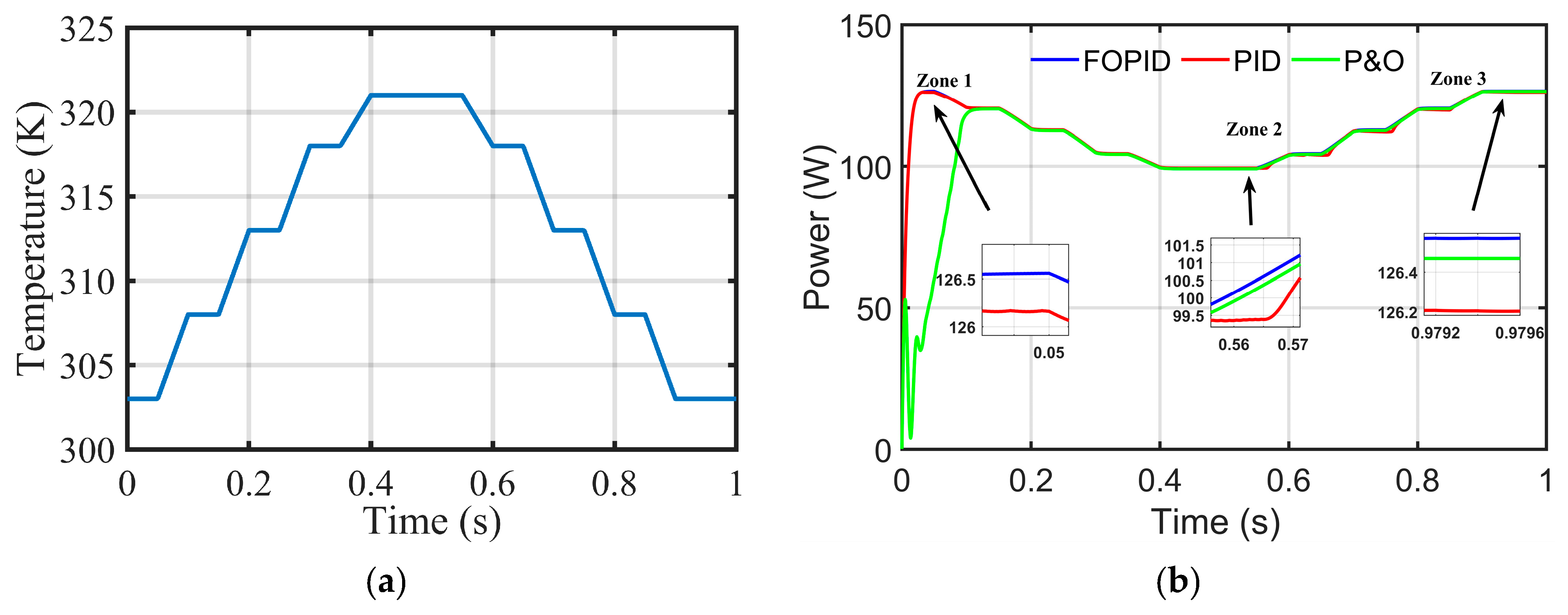
6.1.3. Temperature Variation for Daytime Profile
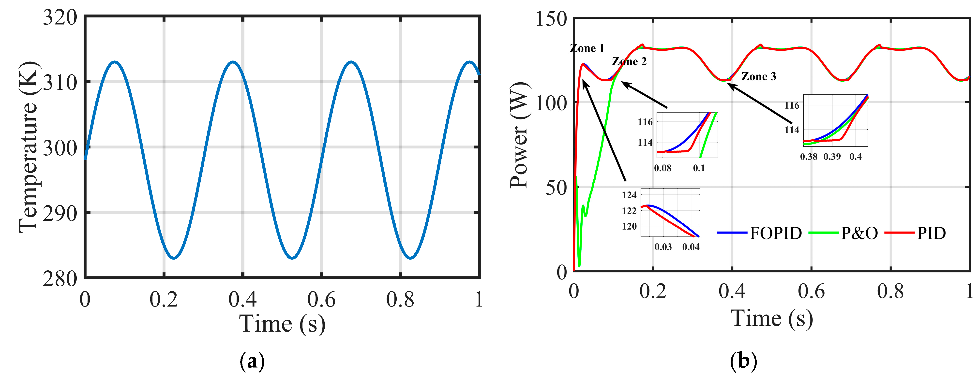
6.1.4. Temperature Variation for Sinusoidal Profile
7. Robustness Test
- Load Variation
- Performance Indices Test
8. Conclusions
Author Contributions
Funding
Conflicts of Interest
Nomenclature
| Variables | Abbreviations | ||
| μ | Differentiator of order | MPP | Maximum power point |
| λ | Integrator of order | PV | Photovoltaic |
| Iph | Photocurrent | PID | Proportional integral derivative |
| Is | Diode saturation current | FOPID | Fractional order proportional integral derivative |
| Rs | Series resistor | AO | Aquila optimizer |
| Rsh | Parallel resistor | MFO | Moth flame optimizer |
| K | Boltzmann constant | P&O | Perturb and observe |
| A | Diode ideality factor | DC | Direct current |
| q | Electron charge | IC | Incremental conductance |
| T | Temperature in Kelvin | FPA | Flower pollination algorithm |
| Ns | Series number of PV cells | PSO | Particle swarm optimizer |
| Np | Parallel number of PV cells | LED | Light-emitting diode |
| V | Output voltage | ANN | Artificial neural network |
| I | Output current | STC | Standard test conditions |
| Vin | Input PV system voltage | SMC | Sliding mode controller |
| Vout | output PV system voltage | FL | Fuzzy logic |
| d | Duty cycle parameter | NPID | Nonlinear proportional integral derivative |
| Kp | Proportional gain | SDM | Single-diode model |
| Ki | Integral gain | IGBT | Insulated gate bipolar transistor |
| Kd | Derivative gain | MOSFET | Metal-oxide-semiconductor field-effect transistor |
| Γ | Euler’s gamma function | ITAE | Integral of time-weighted absolute error |
| X | Population of defined solution | ISE | Integral square error |
| Xi | ith solution position | IAE | Integral absolute error |
| N | Maximum number of populations | ITSE | Integral time square error |
| Dim | Problem dimension space | ||
| rand | Value between 0 and 1 | ||
| LBj | jth minimum limit | ||
| UBj | jth maximum limit | ||
| X1 (t+1) | Solution of the following generation of t | ||
| Xbest (t) | Superior solution of ith generation | ||
| XM | Mean value of location | ||
| XR | Random solution between 1 and N | ||
| D | Dimension search size | ||
| Levy (D) | Levy flight division function | ||
| S | Fixed value of 0.01 | ||
| r1 | Value from 1 to 20 during the search cycles | ||
| U | Value of 0.00565 | ||
| QF(t) | Quality function |
References
- Gao, F.; Hu, R.; Yin, L. Variable boundary reinforcement learning for maximum power point tracking of photovoltaic grid-connected systems. Energy 2023, 264, 126278. [Google Scholar] [CrossRef]
- Farayola, A.M.; Sun, Y.; Ali, A. Global maximum power point tracking and cell parameter extraction in Photovoltaic systems using improved firefly algorithm. Energy Rep. 2022, 8, 162–186. [Google Scholar] [CrossRef]
- Guo, A.; Xu, Y.; Rezvani, A. Performance improvement of maximum power point tracking for photovoltaic system using grasshopper optimization algorithm based ANFIS under different conditions. Optik 2022, 270, 169965. [Google Scholar] [CrossRef]
- Perin Gasparin, F.; Detzel Kipper, F.; Schuck de Oliveira, F.; Krenzinger, A. Assessment on the variation of temperature coefficients of photovoltaic modules with solar irradiance. Sol. Energy 2022, 244, 126–133. [Google Scholar] [CrossRef]
- Osmani, K.; Haddad, A.; Lemenand, T.; Castanier, B.; Ramadan, M. An investigation on maximum power extraction algorithms from PV systems with corresponding DC-DC converters. Energy 2021, 224, 120092. [Google Scholar] [CrossRef]
- Islam, H.; Mekhilef, S.; Shah, N.M.; Soon, T.K.; Wahyudie, A.; Ahmed, M. Improved proportional-integral coordinated MPPT controller with fast tracking speed for grid-tied PV systems under partially shaded conditions. Sustainability 2021, 13, 830. [Google Scholar] [CrossRef]
- Kumar, V.; Bindal, R.K. MPPT technique used with perturb and observe to enhance the efficiency of a photovoltaic system. Mater. Today Proc. 2022, 69, A6–A11. [Google Scholar] [CrossRef]
- Kumar, P.; Shrivastava, A. Maximum power tracking from solar PV system by using fuzzy-logic and incremental conductance techniques. Mater. Today Proc. 2022, 79, 267–277. [Google Scholar] [CrossRef]
- Leelavathi, M.; Suresh Kumar, V. Deep neural network algorithm for MPPT control of double diode equation-based PV module. Mater. Today Proc. 2022, 62, 4764–4771. [Google Scholar] [CrossRef]
- Doubabi, H.; Salhi, I.; Chennani, M.; Essounbouli, N. High Performance MPPT based on TS Fuzzy–integral backstepping control for PV system under rapid varying irradiance—Experimental validation. ISA Trans. 2021, 118, 247–259. [Google Scholar] [CrossRef]
- Srinivasan, V.; Boopathi, C.S.; Sridhar, R. A new meerkat optimization algorithm based maximum power point tracking for partially shaded photovoltaic system. Ain Shams Eng. J. 2021, 12, 3791–3802. [Google Scholar] [CrossRef]
- Pandey, A.K.; Singh, V.; Jain, S. Study and comparative analysis of perturb and observe (P&O) and fuzzy logic based PV-MPPT algorithms. In Applications of AI and IOT in Renewable Energy; Academic Press: Cambridge, MA, USA, 2022. [Google Scholar] [CrossRef]
- Ram, J.P.; Pillai, D.S.; Ghias AM, Y.M.; Rajasekar, N. Performance enhancement of solar PV systems applying P&O assisted Flower Pollination Algorithm (FPA). Sol. Energy 2020, 199, 214–229. [Google Scholar] [CrossRef]
- Dorji, S.; Wangchuk, D.; Choden, T.; Tshewang, T. Maximum power point tracking of solar photovoltaic cell using perturb observe and fuzzy logic controller algorithm for boost converter and quadratic boost converter. Mater. Today Proc. 2020, 27, 1224–1229. [Google Scholar] [CrossRef]
- Mathi, D.K.; Chinthamalla, R. A hybrid global maximum power point tracking method based on butterfly particle swarm optimization and perturb and observe algorithms for a photovoltaic system under partially shaded conditions. Int. Trans. Electr. Energy Syst. 2020, 30, e12543. [Google Scholar] [CrossRef]
- Bhan, V.; Shaikh, S.A.; Khand, Z.H.; Ahmed, T.; Khan, L.A.; Chachar, F.A.; Shaikh, A.M. Performance Evaluation of Perturb and Observe Algorithm for MPPT with Buck–Boost Charge Controller in Photovoltaic Systems. J. Control. Autom. Electr. Syst. 2021, 32, 1652–1662. [Google Scholar] [CrossRef]
- Alagammal, S.; Rathina Prabha, N. Combination of Modified P&O with Power Management Circuit to Exploit Reliable Power from Autonomous PV-Battery Systems. Iran. J. Sci. Technol.-Trans. Electr. Eng. 2021, 45, 97–114. [Google Scholar] [CrossRef]
- Mohammadinodoushan, M.; Abbassi, R.; Jerbi, H.; Ahmed, F.W.; Ahmed, H.A.K.; Rezvani, A. A new MPPT design using variable step size perturb and observe method for PV system under partially shaded conditions by modified shuffled frog leaping algorithm-SMC controller. Sustain. Energy Technol. Assess 2021, 45, 101056. [Google Scholar] [CrossRef]
- Ahmed, N.A.; Abdul Rahman, S.; Alajmi, B.N. Optimal controller tuning for P&O maximum power point tracking of PV systems using genetic and cuckoo search algorithms. Int. Trans. Electr. Energy Syst. 2021, 31, e12624. [Google Scholar] [CrossRef]
- Jiang, M.; Ghahremani, M.; Dadfar, S.; Chi, H.; Abdallah, Y.N.; Furukawa, N. A novel combinatorial hybrid SFL–PS algorithm based neural network with perturb and observe for the MPPT controller of a hybrid PV-storage system. Control Eng. Pract. 2021, 114, 104880. [Google Scholar] [CrossRef]
- Abdel-Salam, M.; El-Mohandes, M.T.; El-Ghazaly, M. An Efficient Tracking of MPP in PV Systems Using a Newly-Formulated P&O-MPPT Method Under Varying Irradiation Levels. J. Electr. Eng. Technol. 2020, 15, 501–513. [Google Scholar] [CrossRef]
- Tali, S.A.; Ahmad, F.; Wani, I.H. Hardware implementation of improved perturb and observe maximum power point tracking technique for photovoltaic systems with zero oscillations. Analog Integr. Circuits Signal Process. 2022, 112, 13–18. [Google Scholar] [CrossRef]
- Siva Kumar, C.H.; Mallesham, G. A new hybrid boost converter with P & O MPPT for high gain enhancement of solar PV system. Mater. Today Proc. 2022, 57, 2262–2269. [Google Scholar] [CrossRef]
- Abdel-Salam, M.; El-Mohandes, M.T.; Goda, M. An improved perturb-and-observe based MPPT method for PV systems under varying irradiation levels. Sol. Energy 2018, 171, 547–561. [Google Scholar] [CrossRef]
- Ali, Z.M.; Vu Quynh, N.; Dadfar, S.; Nakamura, H. Variable step size perturb and observe MPPT controller by applying θ-modified krill herd algorithm-sliding mode controller under partially shaded conditions. J. Clean. Prod. 2020, 271, 122243. [Google Scholar] [CrossRef]
- Ali AI, M.; Mohamed HR, A. Improved P&O MPPT algorithm with efficient open-circuit voltage estimation for two-stage grid-integrated PV system under realistic solar radiation. Int. J. Electr. Power Energy Syst. 2022, 137, 107805. [Google Scholar] [CrossRef]
- Da Rocha, M.V.; Sampaio, L.P.; da Silva SA, O. Comparative analysis of MPPT algorithms based on Bat algorithm for PV systems under partial shading condition. Sustain. Energy Technol. Assess. 2020, 40, 100761. [Google Scholar] [CrossRef]
- Shang, L.; Guo, H.; Zhu, W. An improved MPPT control strategy based on incremental conductance algorithm. Prot. Control Mod. Power Syst. 2020, 5, 14. [Google Scholar] [CrossRef]
- Li, S.; Li, F.; Zheng, J.; Chen, W.; Zhang, D. An improved MPPT control strategy based on incremental conductance method. Soft Comput. 2020, 24, 6039–6046. [Google Scholar] [CrossRef]
- Ahmed, E.M.; Norouzi, H.; Alkhalaf, S.; Ali, Z.M.; Dadfar, S.; Furukawa, N. Enhancement of MPPT controller in PV-BES system using incremental conductance along with hybrid crow-pattern search approach based ANFIS under different environmental conditions. Sustain. Energy Technol. Assess. 2022, 50, 101812. [Google Scholar] [CrossRef]
- Mishra, J.; Das, S.; Kumar, D.; Pattnaik, M. A novel auto-tuned adaptive frequency and adaptive step-size incremental conductance MPPT algorithm for photovoltaic system. Int. Trans. Electr. Energy Syst. 2021, 31, e12813. [Google Scholar] [CrossRef]
- Singh, P.; Shukla, N.; Gaur, P. Modified variable step incremental-conductance MPPT technique for photovoltaic system. Int. J. Inf. Technol. 2021, 13, 2483–2490. [Google Scholar] [CrossRef]
- Sheikh Ahmadi, S.H.; Karami, M.; Gholami, M.; Mirzaei, R. Improving MPPT Performance in PV Systems Based on Integrating the Incremental Conductance and Particle Swarm Optimization Methods. Iran. J. Sci. Technol.-Trans. Electr. Eng. 2022, 46, 27–39. [Google Scholar] [CrossRef]
- Karafil, A. Thinned-out controlled IC MPPT algorithm for class E resonant inverter with PV system. Ain Shams Eng. J. 2023, 14, 101992. [Google Scholar] [CrossRef]
- Jagadeshwar, M.; Dushmanta, K.D. A Novel Adaptive Model Predictive Control Scheme with Incremental Conductance for Extracting Maximum Power from a Solar Panel. Iran. J. Sci. Technol. Trans. Electr. Eng. 2023, 46, 653–664. [Google Scholar] [CrossRef]
- Singh, D.K.; Akella, A.K.; Manna, S. A novel robust maximum power extraction framework for sustainable PV system using incremental conductance based MRAC technique. Environ. Prog. Sustain. Energy 2023, 42, e14137. [Google Scholar] [CrossRef]
- Chauhan, U.; Chhabra, H.; Rani, A.; Kumar, B.; Singh, V. Efficient MPPT Controller for Solar PV System Using GWO-CS Optimized Fuzzy Logic Control and Conventional Incremental Conductance Technique. Iran. J. Sci. Technol.-Trans. Electr. Eng. 2022, 47, 463–472. [Google Scholar] [CrossRef]
- Bouarroudj, N.; Benlahbib, B.; Sedraoui, M.; Feliu-Batlle, V.; Bechouat, M.; Boukhetala, D.; Boudjema, F. A new tuning rule for stabilized integrator controller to enhance the indirect control of incremental conductance MPPT algorithm: Simulation and practical implementation. Optik 2022, 268, 169728. [Google Scholar] [CrossRef]
- Hiyama, T.; Kitabayashi, K. Neural network based estimation of maximum power generation from PV module using environmental information. IEEE Trans. Energy Convers. 1997, 12, 241–247. [Google Scholar] [CrossRef]
- Bahgat AB, G.; Helwa, N.H.; Ahmad, G.E.; el Shenawy, E.T. Maximum power point traking controller for PV systems using neural networks. Renew. Energy 2005, 30, 1257–1268. [Google Scholar] [CrossRef]
- Asiful Islam, M.; Ashfanoor Kabir, M. Neural network based maximum power point tracking of photovoltaic arrays. In IEEE Region 10 Annual International Conference, Proceedings/TENCON; IEEE: Piscataway, NJ, USA, 2011. [Google Scholar] [CrossRef]
- Kurniawan, A.; Shintaku, E. A Neural Network-Based Rapid Maximum Power Point Tracking Method for Photovoltaic Systems in Partial Shading Conditions. Appl. Sol. Energy 2020, 56, 157–167. [Google Scholar] [CrossRef]
- Ibnelouad, A.; el Kari, A.; Ayad, H.; Mjahed, M. Improved cooperative artificial neural network-particle swarm optimization approach for solar photovoltaic systems using maximum power point tracking. Int. Trans. Electr. Energy Syst. 2020, 30, e12439. [Google Scholar] [CrossRef]
- Fathi, M.; Parian, J.A. Intelligent MPPT for photovoltaic panels using a novel fuzzy logic and artificial neural networks based on evolutionary algorithms. Energy Rep. 2021, 7, 1338–1348. [Google Scholar] [CrossRef]
- Hamdi, H.; ben Regaya, C.; Zaafouri, A. Real-time study of a photovoltaic system with boost converter using the PSO-RBF neural network algorithms in a MyRio controller. Sol. Energy 2019, 183, 1–16. [Google Scholar] [CrossRef]
- Rao, C.V.; Raj RD, A.; Anil Naik, K. A novel hybrid image processing-based reconfiguration with RBF neural network MPPT approach for improving global maximum power and effective tracking of PV system. Int. J. Circuit Theory Appl. 2023, 51, 4397–4426. [Google Scholar] [CrossRef]
- Haq, I.U.; Khan, Q.; Ullah, S.; Khan, S.A.; Akmeliawati, R.; Khan, M.A.; Iqbal, J. Neural network-based adaptive global sliding mode MPPT controller design for stand-alone photovoltaic systems. PLoS ONE 2022, 17, e0260480. [Google Scholar] [CrossRef]
- Won, C.Y.; Kim, D.H.; Kim, S.C.; Kim, W.S.; Kim, H.S. New maximum power point tracker of photovoltaic arrays using fuzzy controller. PESC Rec.-IEEE Annu. Power Electron. Spec. Conf. 1994, 1, 396–403. [Google Scholar] [CrossRef]
- Asif, R.M.; Ur Rehman, A.; Ur Rehman, S.; Arshad, J.; Hamid, J.; Tariq Sadiq, M.; Tahir, S. Design and analysis of robust fuzzy logic maximum power point tracking based isolated photovoltaic energy system. Eng. Rep. 2020, 2, e12234. [Google Scholar] [CrossRef]
- Veeramanikandan, P.; Selvaperumal, S. Investigation of different MPPT techniques based on fuzzy logic controller for multilevel DC link inverter to solve the partial shading. Soft Comput. 2021, 25, 3143–3154. [Google Scholar] [CrossRef]
- Senthilnathan, A.; Murugasami, R.; Balakrishnan, R.; Sundar, R.; Palanivel, P. Fuzzy logic controlled 3 port DC to DC Cuk converter with IoT based PV panel monitoring system. Int. J. Syst. Assur. Eng. Manag. 2022, 1–9. [Google Scholar] [CrossRef]
- Hai, T.; Zhou, J.; Muranaka, K. An efficient fuzzy-logic based MPPT controller for grid-connected PV systems by farmland fertility optimization algorithm. Optik 2022, 267, 169636. [Google Scholar] [CrossRef]
- Daraban, S.; Petreus, D.; Morel, C. A novel MPPT (maximum power point tracking) algorithm based on a modified genetic algorithm specialized on tracking the global maximum power point in photovoltaic systems affected by partial shading. Energy 2014, 74, 374–388. [Google Scholar] [CrossRef]
- Hashim, N.; Salam, Z.; Ayob, S.M. Maximum power point tracking for stand-alone photovoltaic system using evolutionary programming. In Proceedings of the 2014 IEEE 8th International Power Engineering and Optimization Conference, PEOCO, Langkawi, Malaysia, 24–25 March 2014. [Google Scholar] [CrossRef]
- Ramasamy, S.; Jeevananthan, S.; Dash, S.S.; Selvan, T. An intelligent differential evolution based maximum power point tracking (MPPT) technique for partially shaded photo voltaic (PV) array. Int. J. Adv. Soft Comput. Its Appl. 2014, 6, 1–16. [Google Scholar]
- Manmadharao, T.; Balamurali, P.; Ravikumar, C. Maximum power point tracking of a PV system by Bacteria foraging oriented Particle Swarm optimization. Int. J. Eng. Res. Gen. Sci. 2015, 3, 515–524. [Google Scholar]
- Ahmed, J.; Salam, Z. A Maximum Power Point Tracking (MPPT) for PV system using Cuckoo Search with partial shading capability. Appl. Energy 2014, 119, 118–130. [Google Scholar] [CrossRef]
- Benyoucef A soufyane Chouder, A.; Kara, K.; Silvestre, S.; Sahed, O.A. Artificial bee colony based algorithm for maximum power point tracking (MPPT) for PV systems operating under partial shaded conditions. Appl. Soft Comput. J. 2015, 32, 38–48. [Google Scholar] [CrossRef]
- Jiang, L.L.; Maskell, D.L.; Patra, J.C. A novel ant colony optimization-based maximum power point tracking for photovoltaic systems under partially shaded conditions. Energy Build. 2013, 58, 227–236. [Google Scholar] [CrossRef]
- Safarudin, Y.M.; Priyadi, A.; Purnomo, M.H.; Pujiantara, M. Maximum power point tracking algorithm for photovoltaic system under partial shaded condition by means updating β firefly technique. In Proceedings of the 2014 6th International Conference on Information Technology and Electrical Engineering: Leveraging Research and Technology Through University-Industry Collaboration, ICITEE, Yogyakarta, Indonesia, 7–8 October 2014. [Google Scholar] [CrossRef]
- Mach, J.B.; Ronoh, K.K.; Langat, K. Improved spectrum allocation scheme for TV white space networks using a hybrid of firefly, genetic, and ant colony optimization algorithms. Heliyon 2023, 9, e13752. [Google Scholar] [CrossRef]
- Lyden, S.; Haque, M.E.; Xiao, D. Application of a Simulated Annealing technique for global maximum power point tracking of PV modules experiencing partial shading. In IECON Proceedings (Industrial Electronics Conference); IEEE: Piscataway, NJ, USA, 2014. [Google Scholar] [CrossRef]
- Mohd Yusof, N.; Muda, A.K.; Pratama, S.F.; Carbo-Dorca, R.; Abraham, A. Improving Amphetamine-type Stimulants drug classification using chaotic-based time-varying binary whale optimization algorithm. Chemom. Intell. Lab. Syst. 2022, 229, 104635. [Google Scholar] [CrossRef]
- Manoochehr Makvandi Neissi, N.; Tarighi, P.; Makvandi, K.; Rashidi, N. Evaluation of the Genes Expression Related to the Immune System in Response to Helicobacter pylori Catalase Epitopes. Mol. Genet. Microbiol. Virol. 2020, 35, 47–51. [Google Scholar] [CrossRef]
- Barr, R.S.; Glover, F.; Huskinson, T.; Kochenberger, G. An extreme-point tabu-search algorithm for fixed-charge network problems. Networks 2021, 77, 322–340. [Google Scholar] [CrossRef]
- Saleem, O.; Awan, F.G.; Mahmood-ul-Hasan, K.; Ahmad, M. Self-adaptive fractional-order LQ-PID voltage controller for robust disturbance compensation in DC-DC buck converters. Int. J. Numer. Model. 2020, 33, e2718. [Google Scholar] [CrossRef]
- Youcef, D.; Khatir, K.; Yassine, B. Design of neural network fractional-order backstepping controller for MPPT of PV systems using fractional-order boost converter. Int Trans Electr Energ Syst. 2021, 31, e13188. [Google Scholar] [CrossRef]
- Chen, X.; Chen, Y.; Zhang, B.; Qiu, D. A modeling and analysis method for fractional-order DC–DC converters. IEEE Trans. Power Electron. 2016, 32, 7034–7044. [Google Scholar] [CrossRef]
- Ni, J.; Xiang, J. A Concise Control Method Based on Spatial-Domain dp/dv Calculation for MPPT/Power Reserved of PV Systems. IEEE Trans. Energy Convers. 2023, 38, 3–14. [Google Scholar] [CrossRef]
- Park, H.E.; Song, J.H. A dP/dV feedback-controlled MPPT method for photovoltaic power system using II-SEPIC. J. Power Electron. 2009, 9, 604–611. [Google Scholar]
- Dounis, A.I.; Kofinas, P.; Alafodimos, C.; Tseles, D. Adaptive fuzzy gain scheduling PID controller for maximum power point tracking of photovoltaic system. Renew. Energy 2013, 60, 202–214. [Google Scholar] [CrossRef]
- Dounis, A.I.; Stavrinidis, S.; Kofinas, P.; Tseles, D. Fuzzy-PID controller for MPPT of PV system optimized by Big Bang-Big Crunch algorithm. In Proceedings of the IEEE International Conference on Fuzzy Systems, Istanbul, Turkey, 2–5 November 2015. [Google Scholar] [CrossRef]
- Ashok Kumar, B.; Srinivasa Venkatesh, M.; Mohan Muralikrishna, G. Optimization of photovoltaic power using PID MPPT controller based on incremental conductance algorithm. Lect. Notes Electr. Eng. 2015, 326, 803–809. [Google Scholar] [CrossRef]
- Kler, D.; Rana KP, S.; Kumar, V. A nonlinear PID controller based novel maximum power point tracker for PV systems. J. Frankl. Inst. 2018, 355, 7827–7864. [Google Scholar] [CrossRef]
- Long, B.; Lu, P.; Zhan, D.; Lu, X.; Rodríguez, J.; Guerrero, J.M.; Chong, K. Adaptive fuzzy fractional-order sliding-mode control of LCL-interfaced grid-connected converter with reduced-order. ISA Trans. 2023, 132, 557–572. [Google Scholar] [CrossRef]
- Ahmed, W.A.E.M.; Mageed, H.M.A.; Mohamed, S.A.E.; Saleh, A.A. Fractional order Darwinian particle swarm optimization for parameters identification of solar PV cells and modules. Alex. Eng. J. 2022, 61, 1249–1263. [Google Scholar] [CrossRef]
- Yang, B.; Yu, T.; Shu, H.; Zhu, D.; An, N.; Sang, Y.; Jiang, L. Perturbation observer based fractional-order sliding-mode controller for MPPT of grid-connected PV inverters: Design and real-time implementation. Control. Eng. Pract. 2018, 79, 105–125. [Google Scholar] [CrossRef]
- Monje C a Chen, Y.Q.; Vinagre, B.M.; Xue, D.; Feliu, V. Fractional-order Systems and Controls. Fundamentals and Applications; Springer-Verlag: London, UK, 2010. [Google Scholar] [CrossRef]
- Raheem, F.S.; Basil, N. Automation intelligence photovoltaic system for power and voltage issues based on Black Hole Optimization algorithm with FOPID. Meas. Sens. 2023, 25, 100640. [Google Scholar] [CrossRef]
- Abualigah, L.; Yousri, D.; Abd Elaziz, M.; Ewees, A.A.; Al-qaness MA, A.; Gandomi, A.H. Aquila Optimizer: A novel meta-heuristic optimization algorithm. Comput. Ind. Eng. 2021, 157, 107250. [Google Scholar] [CrossRef]


| MPPT Approach | Application | Complexity Level | Convergence Rapidity | Noticed Parameters | Preceding Training | Cost | Efficiency |
|---|---|---|---|---|---|---|---|
| P&O [12,16] | Stand-alone | Modest | Alternates | Current Voltage | None | Low | Up to 95% |
| IC [28,29] | Stand-alone | Intermediate | Alternates | Current Voltage | None | Low | Up to 97% |
| ANN [39,40,41] | Both | Advanced | Rapid | Relates | Yes | High | Up to 98% |
| FL [48,49] | Both | Advanced | Rapid | Relates | None | High | Up to 98% |
| SMC [25] | Both | Advanced | Rapid | Relates | None | High | Up to 98% |
| Optimization approaches [53,54,55,56,57,58,59,60,61,62,63,64,65] | Both | Advanced | Rapid | Relates | None | High | Up to 98% |
| Hybrid techniques [38,47,50] | Both | Advanced | Rapid | Relates | None | High | Up to 98% |
| dp/dv feedback-control-based PID [73] | Both | Intermediate | Rapid | Voltage Power | None | Medium | Up to 98% |
| dp/dv feedback-control-based NFOPID [75] | Both | Advanced | Rapid | Voltage Power | None | Medium | Up to 98% |
| Parameter | Value |
|---|---|
| Iph (A) | 8.0428 |
| Is (A) | 2.2655 × 10⁻¹⁰ |
| Rs (Ω) | 0.22151 |
| Rsh (Ω) | 78.0854 |
| A | 0.97611 |
| Ns | 36 |
| Np | 1 |
| FOPID Parameter | PID Parameter | Lower Range | Higher Range |
|---|---|---|---|
| 0.001 | 100 | ||
| 0.001 | 100 | ||
| 0.001 | 100 | ||
| - | 0.100 | 0.95 | |
| - | 0.1 | 0.95 |
| Controller | Proposed Algorithms | Fitness Value | |||||
|---|---|---|---|---|---|---|---|
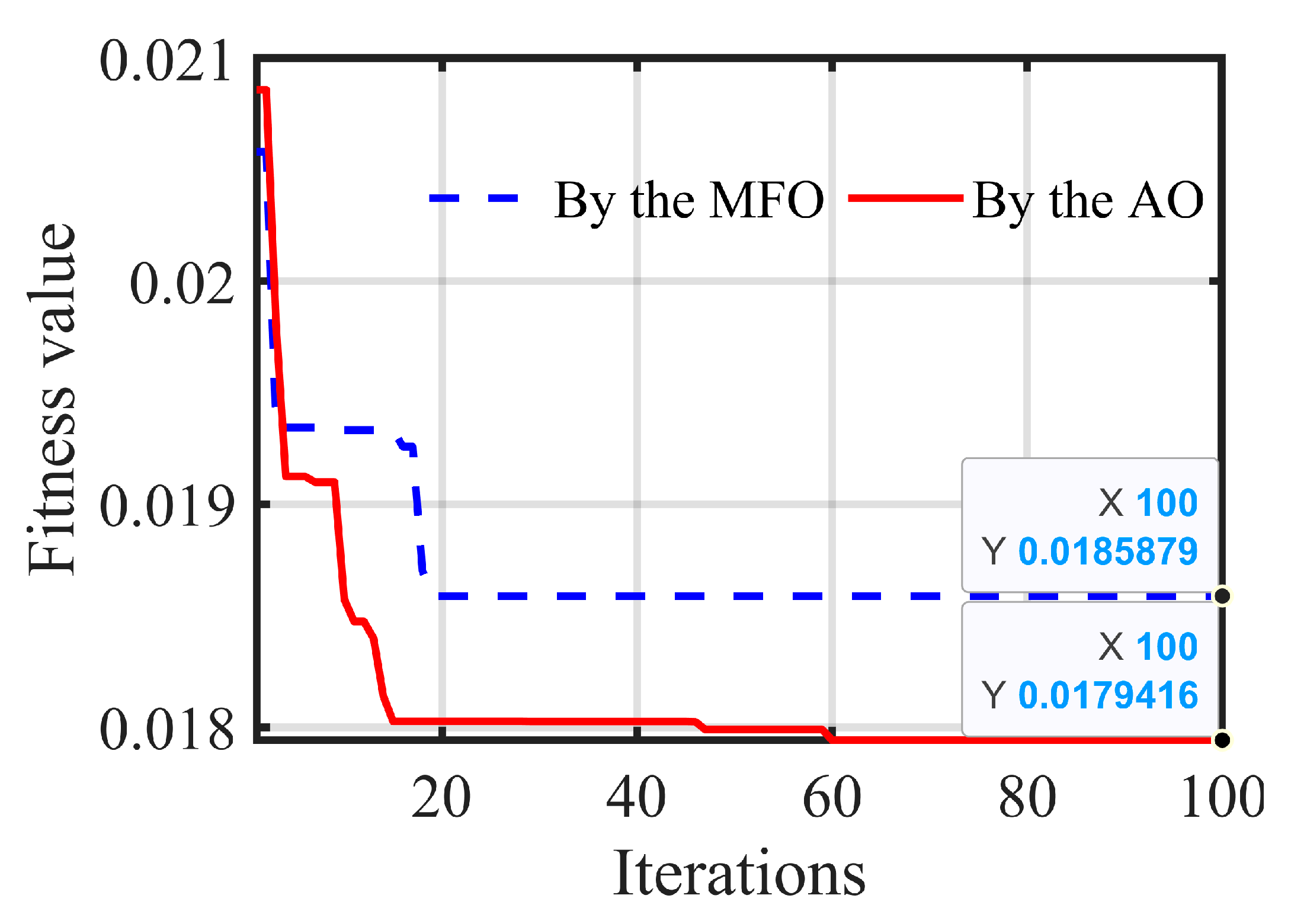
| FOPD | AO | 69.6734 | 100.0000 | 0.0010 | 0.6398 | 0.5502 | 0.0179 |
| MFO | 25.3656 | 99.9312 | 15.8049 | 0.5809 | 0.1000 | 0.0185 |
| Proposed Algorithms | Controllers | Fitness Value | |||||
|---|---|---|---|---|---|---|---|
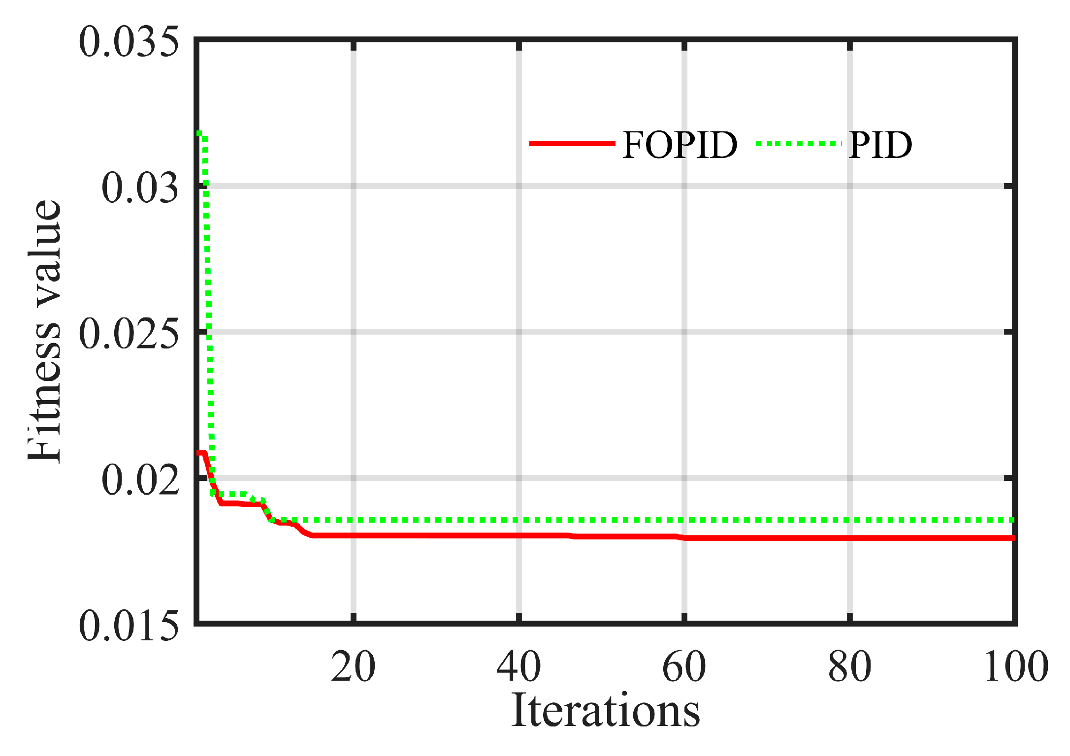
| AO | FOPID | 69.6734 | 100 | 0.0010 | 0.6398 | 0.5502 | 0.0179 |
| PID | 93.0756 | 100 | 0.0010 | - | - | 0.0186 |
| PI | Zone | FOPID | PID | P&O |
|---|---|---|---|---|
| Overshoot (W) | 1 | - | - | - |
| 2 | 2.9346 × 10⁻⁴ | 0.1486 | 2.1457 × 10⁻³ | |
| 3 | 0.0031 | 0.0040 | 0.0044 | |
| 4 | 0.0147 | 0.0147 | 0.0180 |
| PI | FOPID | PID | P&O |
|---|---|---|---|
| Overshoot (W) | 4.5088 × 10⁻⁴ | 5.0118 × 10⁻⁴ | Out of zone |
| PI | FOPID | PID | P&O |
|---|---|---|---|
| Overshoot (W) | 2.3340 | 2.5665 | Out of zone |
| PI | FOPID | PID | P&O |
|---|---|---|---|
| Overshoot (W) | 5.0186 | 5.0980 | Out of zone |
| Controllers | ISE | IAE | ITSE | ITAE | |
|---|---|---|---|---|---|
| Irradiation variation for daytime profile | P&O | 0.0101 | 0.0283 | 0.0026 | 0.0073 |
| PID | 0.0264 | 0.0452 | 0.0068 | 0.0117 | |
| FOPID | 0.0015 | 0.0109 | 3.8856 × 10⁻⁴ | 0.0028 | |
| Temperature variation for daytime profile | P&O | 0.0028 | 0.0110 | 0.0017 | 0.0068 |
| PID | 0.0061 | 0.0169 | 0.0038 | 0.0106 | |
| FOPID | 3.3339 × 10⁻⁴ | 0.0035 | 2.0605 × 10⁻⁴ | 0.0022 |
Disclaimer/Publisher’s Note: The statements, opinions and data contained in all publications are solely those of the individual author(s) and contributor(s) and not of MDPI and/or the editor(s). MDPI and/or the editor(s) disclaim responsibility for any injury to people or property resulting from any ideas, methods, instructions or products referred to in the content. |
© 2023 by the authors. Licensee MDPI, Basel, Switzerland. This article is an open access article distributed under the terms and conditions of the Creative Commons Attribution (CC BY) license (https://creativecommons.org/licenses/by/4.0/).
Share and Cite
Tadj, M.; Chaib, L.; Choucha, A.; Aldaoudeyeh, A.-M.; Fathy, A.; Rezk, H.; Louzazni, M.; El-Fergany, A. Enhanced MPPT-Based Fractional-Order PID for PV Systems Using Aquila Optimizer. Math. Comput. Appl. 2023, 28, 99. https://doi.org/10.3390/mca28050099
Tadj M, Chaib L, Choucha A, Aldaoudeyeh A-M, Fathy A, Rezk H, Louzazni M, El-Fergany A. Enhanced MPPT-Based Fractional-Order PID for PV Systems Using Aquila Optimizer. Mathematical and Computational Applications. 2023; 28(5):99. https://doi.org/10.3390/mca28050099
Chicago/Turabian StyleTadj, Mohammed, Lakhdar Chaib, Abdelghani Choucha, Al-Motasem Aldaoudeyeh, Ahmed Fathy, Hegazy Rezk, Mohamed Louzazni, and Attia El-Fergany. 2023. "Enhanced MPPT-Based Fractional-Order PID for PV Systems Using Aquila Optimizer" Mathematical and Computational Applications 28, no. 5: 99. https://doi.org/10.3390/mca28050099