Global Behavior of Solutions to a Higher-Dimensional System of Difference Equations with Lucas Numbers Coefficients

Abstract

In this paper, we derive the well-defined solutions to a $\theta$-dimensional system of difference equations. We show that, the well-defined solutions to that system are represented in terms of Fibonacci and Lucas sequences. Moreover, we study the global stability of the solutions to that system. Finally, we give some numerical examples which confirm our theoretical results.

1. Introduction

Difference equations and systems of difference equations are of great importance in the field of mathematics as well as in other sciences. The applications of the difference equations appear as discrete mathematical models of many phenomena such as in biology, economics, ecology, control theory, physics, engineering, population dynamics and so forth [1,2,3,4,5,6]. This is the reason why, recently, many scientists have devoted their work to the study of the theory of difference equations, the boundedness, the periodicity and the global asymptotic stability of their solutions [7,8,9,10,11,12,13,14,15,16,17,18,19,20,21,22,23,24,25,26,27,28,29,30,31].

In the following, we will use the following notations: $\mathbb{N}$ for the set of natural numbers, and ${\mathbb{N}}_{\nu }$ for the set $\{n\in \mathbb{Z}:n\ge \nu \}$. Recently, there has been a growing interest in the study of finding closed-form solutions of difference equations and systems of difference equations. Some of the forms of solutions of these equations are representable via well-known integer sequences such as Fibonacci numbers (see, for example [26,32]), Horadam numbers (see, for example, [30,31]), Lucas numbers (see, for example [25,27,33]), Pell numbers and Padovan numbers (see, for example [34,35,36]), But in this paper, we present the solution in the form of Lucas sequences.

In [32], the authors represented the general solution of the following difference equation

$$x_{n+1}={\displaystyle \frac{1}{1+x_n}},n\in {\mathbb{N}}_0,$$

(1)

in terms of the initial value $x_0$ and the Fibonacci sequence. Namely, it was proved by induction that every well-defined solution of Equation (1) can be written in the following form

$$x_n={\displaystyle \frac{F_n+F_{n-1}{x}_0}{F_{n+1}+F_n{x}_0}},n\in {\mathbb{N}}_0,$$

where ${\left\{F_n\right\}}_{n=0}^{\infty }$ is Fibonacci sequence. They also proved that, every well-defined solution of the equation

$$x_{n+1}={\displaystyle \frac{1}{-1+x_n}},n\in {\mathbb{N}}_0,$$

(2)

can be written in the following form

$$x_n={\displaystyle \frac{F_{-n}+F_{-(n-1)}{x}_0}{F_{-(n+1)}+F_{-n}{x}_0}},n\in {\mathbb{N}}_0,$$

where the terms of the Fibonacci sequence with negative indices are calculated by the formula

$$F_{-n}=F_{-n+2}-F_{-n+1},n\in {\mathbb{N}}_0,$$

with $F_0=0$ and $F_1=1$.

Stevic [30] represented the general solution of the following bilinear system of difference equations

$$x_{n+1}={\displaystyle \frac{\alpha +\beta y_n}{\gamma +\sigma y_n}},y_{n+1}={\displaystyle \frac{\alpha +\beta x_n}{\gamma +\sigma x_n}},$$

in terms of the initial values $x_0$, $y_0$ and the generalized Fibonacci sequence.

In [26], Khelifa and Halim analyzed the general solution to the system of difference equations

$$x_{n+1}^{\left(j\right)}={\displaystyle \frac{F_{m+2}+F_{m+1}{x}_{n-k}^{\left(\right(j+1)mod(p\left)\right)}}{F_{m+3}+F_{m+2}{x}_{n-k}^{\left(\right(j+1)mod(p\left)\right)}}},$$

where $n,m\in {\mathbb{N}}_0$, $j=1,\dots ,p$, and ${\left(F_n\right)}_{n=0}^{+\infty }$ is Fibonacci sequence. They expressed the solution to this system in terms of the Fibonacci sequence.

In this paper, we derive the well-defined solutions to the $\theta$-dimensional system of difference equations of the form

$$x_{n+1}^{\left(q\right)}={\displaystyle \frac{L_{m+2}+L_{m+1}{x}_{n-k}^{\left(\right(q+1)mod(\theta \left)\right)}}{L_{m+3}+L_{m+2}{x}_{n-k}^{\left(\right(q+1)mod(\theta \left)\right)}}},n\in {\mathbb{N}}_0,$$

(3)

where $k\in {\mathbb{N}}_0$, $m\in \mathbb{Z}$, $q=1,\cdots ,\theta$, $\theta \in \mathbb{N}$, ${\left(L_n\right)}_{n=0}^{+\infty }$ is Lucas sequence, and the initial values $x_{-i}^{\left(q\right)}$, $i=0,\dots ,k$ are real numbers, $q=1,\dots ,\theta$.

Clearly, our system generalizes the equations and systems studied in [25,27,32,33].

2. Preliminaries

Fibonacci sequence [6,37] is defined by

$$F_{n+1}=F_n+F_{n-1},n\in \mathbb{N},$$

(4)

where $F_0=0$ and $F_1=1$. The solution to Equation (4) is given by the Binet formula of Fibonacci sequence is given by

$$F_n=\frac{{\alpha }^n-{\beta }^n}{\alpha -\beta },$$

where

$$\alpha ={\displaystyle \frac{1+\sqrt{5}}{2}},\beta ={\displaystyle \frac{1-\sqrt{5}}{2}}.$$

Here, $\alpha$ is the so-called golden number.

Lucas sequence is the sequence of integer numbers defined by the recurrence relation

$$L_{n+1}=L_n+L_{n-1},n\in \mathbb{N},$$

(5)

with initial conditions $L_0=2$ and $L_1=1$. The Binet formula for the Lucas sequence is given by

$$L_n={\alpha }^n+{\beta }^n.$$

The formula of terms with negative indices in the Lucas sequence is

$$L_{-n}={(-1)}^n{L}_n,n=1,2,\cdots .$$

Now, we list a set of properties concerning Fibonacci and Lucas sequences that will be used through the paper [6,37].

Propertiesn 1.

Suppose that ${\left(F_n\right)}_{n=0}^{+\infty }$ and ${\left(L_n\right)}_{n=0}^{+\infty }$ are Fibonacci and Lucas sequences, and let $\eta ,\kappa \in \mathbb{N}$. Then

1. 

$L_{\eta +1}{L}_{(\kappa -1)\eta }+L_{\eta }{L}_{(\kappa -1)\eta -1}=5F_{\kappa \eta },$

2. 

$L_{\eta }{L}_{(\kappa -1)\eta }+L_{\eta -1}{L}_{(\kappa -1)\eta -1}=5F_{\kappa \eta -1},$

3. 

$F_{\kappa +1}{L}_{\eta -\kappa }+F_{\kappa }{L}_{\eta -(\kappa +1)}=L_{\eta },$

4. 

$F_{\kappa }{L}_{\eta +3}+F_{\kappa -1}{L}_{\eta +2}=L_{\kappa +\eta +2},$

5. 

$L_{\kappa (\eta +2)-1}+L_{\kappa (\eta +2)+1}=5F_{\kappa (\eta +2)},$

6. 

$L_{\kappa (\eta +2)}^2-L_{\kappa (\eta +2)-1}{L}_{\kappa (\eta +2)+1}=5{(-1)}^{\kappa (\eta +2)},$

7. 

$L_{\kappa }{L}_{\eta -(\kappa -1)}+L_{(\kappa -1)}{L}_{\eta -\kappa }=5F_{\eta },$

8. 

$F_{\kappa }{F}_{\eta -(\kappa -1)}+F_{\kappa -1}{F}_{\eta -\kappa }=F_{\eta },$

Propertiesn 2.

Suppose that ${\left(F_n\right)}_{n=0}^{+\infty }$ and ${\left(L_n\right)}_{n=0}^{+\infty }$ are Fibonacci and Lucas sequences, and let $\eta ,\kappa \in \mathbb{N}$. Then

1. 

$5F_{2\kappa \eta }+{(-1)}^{\kappa }{L}_{\kappa +1}{L}_{\kappa (2\eta +1)}={(-1)}^{\kappa }{L}_{\kappa }{L}_{\kappa (2\eta +1)+1},$

2. 

$L_{\kappa (2\eta +1)}-L_{\kappa +1}{F}_{2\kappa \eta }=L_{\kappa }{F}_{2\kappa \eta -1},$

3. 

$L_{\kappa (2\eta -1)-1}+{(-1)}^{\kappa }{L}_{\kappa +1}{F}_{2\kappa \eta -1}={(-1)}^{\kappa }{L}_{\kappa }{F}_{2\kappa \eta },$

Theorem 3

([26]). Let ${\left(u_n\right)}_{n\ge -\theta +1}$ be a solution to Equation

$$u_{n+1}={\displaystyle \frac{F_{\theta (m+2)}+F_{\theta (m+2)-1}{u}_{n-(\theta -1)}}{F_{\theta (m+2)+1}+F_{\theta (m+2)}{u}_{n-(\theta -1)}}},n\in {\mathbb{N}}_0.$$

(6)

Then for $n\in {\mathbb{N}}_0$,

$$u_{\theta n+j}={\displaystyle \frac{F_{\theta n(m+2)}+F_{\theta n(m+2)-1}{u}_j}{F_{\theta n(m+2)+1}+F_{\theta n(m+2)}{u}_j}},$$

where $\theta ,m\in \mathbb{N}$, $j\in \{0,1,\cdots ,\theta -1\}$.

Proof. 

The proof of this theorem can be found in [26], where it is similar to Equation (17) there. □

3. Main Results

In this section, we establish the form of the solution to system (3).

Using the transformation

$$X_n^{\left(q\right)}=x_{(k+1)n-t}^{\left(q\right)},n\in {\mathbb{N}}_0,$$

(7)

where $t\in \{0,1,\dots ,k\}$ and $q\in \{1,2,\dots ,\theta \}$, we can write system (3) as

$$\begin{array}{ccc}\hfill X_{n+1}^{\left(1\right)}& =& \frac{L_{m+2}+L_{m+1}{X}_n^{\left(2\right)}}{L_{m+3}+L_{m+2}{X}_n^{\left(2\right)}},\hfill \\ \hfill X_{n+1}^{\left(2\right)}& =& \frac{L_{m+2}+L_{m+1}{X}_n^{\left(3\right)}}{L_{m+3}+L_{m+2}{X}_n^{\left(3\right)}},\hfill \\ & ⋮& \hfill \\ \hfill X_{n+1}^{\left(\theta \right)}& =& \frac{L_{m+2}+L_{m+1}{X}_n^{\left(1\right)}}{L_{m+3}+L_{m+2}{X}_n^{\left(1\right)}},n\in {\mathbb{N}}_0.\hfill \end{array}$$

(8)

3.1. Solvability of System (8)

In this section, we shall derive the solution to system (8).

If we use the second recurrence relation in system (8) in the first, we obtain

$$X_{n+1}^{\left(1\right)}={\displaystyle \frac{F_{2m+4}+F_{2m+3}{X}_{n-1}^{\left(3\right)}}{F_{2m+5}+F_{2m+4}{X}_{n-1}^{\left(3\right)}}},n\ge 1.$$

The substitution of $X_{n-1}^{\left(3\right)}$ into $X_{n+1}^{\left(1\right)}$ leads to

$$X_{n+1}^{\left(1\right)}={\displaystyle \frac{L_{3m+6}+L_{3m+5}{X}_{n-2}^{\left(4\right)}}{L_{3m+7}+L_{3m+6}{X}_{n-2}^{\left(4\right)}}},n\ge 2.$$

Similarly, if we replace $X_{n-1}^{\left(4\right)}$ into $X_{n+1}^{\left(1\right)}$, we get

$$X_{n+1}^{\left(1\right)}={\displaystyle \frac{F_{4m+8}+F_{4m+7}{x}_{n-3}^{\left(5\right)}}{F_{4m+9}+F_{4m+8}{X}_{n-3}^{\left(5\right)}}},n\ge 3.$$

Proceeding in the same manner, and using Property 1, system (8) can be written in the following form:

$$X_{n+1}^{\left(1\right)}={\displaystyle \frac{F_{2p(m+2)}+F_{2p(m+2)-1}{X}_{n-(2p-1)}^{\left(1\right)}}{F_{2p(m+2)+1}+F_{2p(m+2)}{X}_{n-(2p-1)}^{\left(1\right)}}},n\ge 2p-1,$$

(9)

when $\theta =2p$, and

$$X_{n+1}^{\left(1\right)}={\displaystyle \frac{L_{(2p+1)(m+2)}+L_{(2p+1)(m+2)-1}{X}_{n-2p}^{\left(1\right)}}{L_{(2p+1)(m+2)+1}+L_{(2p+1)(m+2)}{X}_{n-2p}^{\left(1\right)}}},n\ge 2p,$$

(10)

when $\theta =2p+1$, where $p\in \mathbb{N}$.

3.1.1. Case $\theta =2p$

Here, we consider the case $\theta =2p$. Using Theorem 3, the solution of Equation (9) can be written as

$$X_{2pn+j}^{\left(1\right)}={\displaystyle \frac{F_{2pn(m+2)}+F_{2pn(m+2)-1}{X}_j^{\left(1\right)}}{F_{2pn(m+2)+1}+F_{2pn(m+2)}{X}_j^{\left(1\right)}}},n\in {\mathbb{N}}_0,$$

where $p\in \mathbb{N}$, $m\in \mathbb{Z}$ and $j\in \{0,1,\cdots ,2p\}$.

Theorem 4.

Let ${\left(X_n^{\left(1\right)},X_n^{\left(2\right)},\dots ,X_n^{\left(2p\right)}\right)}_{n\ge 0}$ be a solution to system (8). Then

$$X_{2pn+j}^{\left(q\right)}={\displaystyle \frac{L_{2p(m+2)n+j(m+2)}+L_{2p(m+2)n+j(m+2)-1}{X}_0^{\left(s\right)}}{L_{2p(m+2)n+j(m+2)+1}+L_{2p(m+2)n+j(m+2)}{X}_0^{\left(s\right)}}},j\in \{1,3,\dots ,2p-1\},$$

and

$$X_{2pn+j}^{\left(q\right)}={\displaystyle \frac{F_{2p(m+2)n+j(m+2)}+F_{2p(m+2)n+j(m+2)-1}{X}_0^{\left(s\right)}}{F_{2p(m+2)n+j(m+2)+1}+F_{2p(m+2)n+j(m+2)}{X}_0^{\left(s\right)}}},j\in \{0,2,\dots ,2p-2\},$$

where $n\in {\mathbb{N}}_0$, $s=(q+j)mod\left(2p\right)$ and $q\in \{1,2,\dots ,2p\}$.

Proof. 

Let ${\left(X_n^{\left(1\right)},X_n^{\left(2\right)},\dots ,X_n^{2p}\right)}_{n\ge 0}$ be a solution to system (8). Then

$$X_{2pn+j}^{\left(1\right)}={\displaystyle \frac{F_{2pn(m+2)}+F_{2pn(m+2)-1}{X}_j^{\left(1\right)}}{F_{2pn(m+2)+1}+F_{2pn(m+2)}{X}_j^{\left(1\right)}}},n\in {\mathbb{N}}_0.$$

(11)

We consider two different situations, depending on whether j is even or odd.

• When j is odd, we have that

  $$X_j^{\left(1\right)}={\displaystyle \frac{L_{j(m+2)}+L_{j(m+2)-1}{X}_0^{(1+j)}}{L_{j(m+2)+1}+L_{j(m+2)}{X}_0^{(1+j)}}}.$$
  This implies that for $j\in \{1,3,\cdots ,2p-1\}$ we get

  $$\begin{array}{cc}\hfill X_{2pn+j}^{\left(1\right)}=& {\displaystyle \frac{(L_{j(m+2)+1}+L_{j(m+2)}{X}_0^{(1+j)})L_{2p(m+2)n+j(m+2)-j(m+2)}}{(L_{j(m+2)+1}+L_{j(m+2)}{X}_0^{(1+j)})L_{2p(m+2)n+j(m+2)-j(m+2)+1}}}\hfill \\ & {\displaystyle \frac{+(L_{j(m+2)}+L_{j(m+2)-1}{X}_0^{(1+j)})L_{2p(m+2)n+j(m+2)-j(m+2)-1}}{+(L_{j(m+2)}+L_{j(m+2)-1}{X}_0^{(1+j)})L_{2p(m+2)n+j(m+2)-j(m+2)}},}\hfill \\ \hfill =& {\displaystyle \frac{L_{2p(m+2)n+j(m+2)}+L_{2p(m+2)n+j(m+2)-1}{X}_0^{(1+j)}}{L_{2p(m+2)n+j(m+2)+1}+L_{2p(m+2)n+j(m+2)}{X}_0^{(1+j)}}}.\hfill \end{array}$$
• Similarly, for $j\in \{0,2,\cdots ,2p-2\}$, we get

  $$X_{2pn+j}^{\left(1\right)}={\displaystyle \frac{F_{2p(m+2)n+j(m+2)}+F_{2p(m+2)n+j(m+2)-1}{X}_0^{(1+j)}}{F_{2p(m+2)n+j(m+2)+1}+F_{2p(m+2)n+j(m+2)}{X}_0^{(1+j)}}}.$$

Then for the solution ${\left(X_n^{\left(1\right)},X_n^{\left(2\right)},\dots ,X_n^{\left(2p\right)}\right)}_{n\ge 0}$, we can write

$$X_{2pn+j}^{\left(q\right)}={\displaystyle \frac{L_{2p(m+2)n+j(m+2)}+L_{2p(m+2)n+j(m+2)-1}{X}_0^{\left(s\right)}}{L_{2p(m+2)n+j(m+2)+1}+L_{2p(m+2)n+j(m+2)}{X}_0^{\left(s\right)}}},j\in \{1,3,\dots ,2p-1\},$$

and

$$X_{2pn+j}^{\left(q\right)}={\displaystyle \frac{F_{2p(m+2)n+j(m+2)}+F_{2p(m+2)n+j(m+2)-1}{X}_0^{\left(s\right)}}{F_{2p(m+2)n+j(m+2)+1}+F_{2p(m+2)n+j(m+2)}{X}_0^{\left(s\right)}}},j\in \{0,2,\dots ,2p-2\},$$

where $n\in {\mathbb{N}}_0$, $s=(q+j)mod\left(2p\right)$ and $q\in \{1,2,\dots ,2p\}$.

This completes the proof. □

Using the preceding arguments, we can provide the main result for the solvability of system (3).

Theorem 5. 

Assume that $\theta =2p$ and let ${\left(x_n^{\left(1\right)},x_n^{\left(2\right)},\dots ,x_n^{\left(2p\right)}\right)}_{n\ge -k}$ be a solution to system (3). Then, for all $q\in \{1,2,\dots ,2p\}$, the solution to system (3) is

$$\begin{array}{ccc}\hfill x_{(k+1)(2pn+j)-t}^{\left(q\right)}& =& {\displaystyle \frac{L_{2p(m+2)n+j(m+2)}+L_{2p(m+2)n+j(m+2)-1}{x}_{-t}^{\left(\right(q+j)mod(2p\left)\right)}}{L_{2p(m+2)n+j(m+2)+1}+L_{2p(m+2)n+j(m+2)}{x}_{-t}^{\left(\right(q+j)mod(2p\left)\right)}}},\hfill \end{array}$$

for $j\in \{1,3,\cdots ,2p-1\}$, and

$$\begin{array}{ccc}\hfill x_{(k+1)(2pn+j)-t}^{\left(q\right)}& =& {\displaystyle \frac{F_{2p(m+2)n+j(m+2)}+F_{2p(m+2)n+j(m+2)-1}{x}_{-t}^{\left(\right(q+j)mod(2p\left)\right)}}{F_{2p(m+2)n+j(m+2)+1}+F_{2p(m+2)n+j(m+2)}{x}_{-t}^{\left(\right(q+j)mod(2p\left)\right)}}},\hfill \end{array}$$

for $j\in \{0,2,\dots ,2p-2\}$, where $t\in \{0,1,\cdots ,k\}$.

3.1.2. Case $\theta =2p+1$

Here, we consider the case $\theta =2p+1$.

Using the transformation

$${\mathsf{\Psi }}_n^j=X_{(2p+1)n+j}^{\left(1\right)},n\in {\mathbb{N}}_0,$$

(12)

where $j\in \{0,1,2,\cdots ,2p\}$, we can write Equation (10) in the form

$${\mathsf{\Psi }}_{n+1}^j={\displaystyle \frac{L_{(2p+1)(m+2)}+L_{(2p+1)(m+2)-1}{\mathsf{\Psi }}_n^j}{L_{(2p+1)(m+2)+1}+L_{(2p+1)(m+2)}{\mathsf{\Psi }}_n^j}},n\in {\mathbb{N}}_0,$$

(13)

where $j\in \{0,1,2,\cdots ,2p\}$.

From Appendix A, the solution to Equation (13) is given by

$$\begin{array}{ccc}\hfill {\mathsf{\Psi }}_{2n}^j& =& {\displaystyle {\displaystyle \frac{F_{2(2p+1)(m+2)n}+F_{2(2p+1)(m+2)n-1}{\mathsf{\Psi }}_0^j}{F_{2(2p+1)(m+2)n+1}+F_{2(2p+1)(m+2)n}{\mathsf{\Psi }}_0^j}},n\in {\mathbb{N}}_0,}\hfill \\ \hfill {\mathsf{\Psi }}_{2n+1}^j& =& {\displaystyle {\displaystyle \frac{L_{(2p+1)(m+2)(2n+1)}+L_{(2p+1)(m+2)(2n+1)-1}{\mathsf{\Psi }}_0^j}{L_{(2p+1)(m+2)(2n+1)+1}+L_{(2p+1)(m+2)(2n+1)}{\mathsf{\Psi }}_0^j}},n\in {\mathbb{N}}_0,}\hfill \end{array}$$

where $j\in \{0,1,\cdots ,2p\}.$

Therefore, the solution to Equation (10) is

$$\begin{array}{ccc}\hfill X_{2(2p+1)n+j}^{\left(1\right)}& =& {\displaystyle \frac{F_{2(2p+1)(m+2)n}+F_{2(2p+1)(m+2)n-1}{X}_j^{\left(1\right)}}{F_{2(2p+1)(m+2)n+1}+F_{2(2p+1)(m+2)n}{X}_j^{\left(1\right)}}},\hfill \\ \hfill X_{(2p+1)(2n+1)+j}^{\left(1\right)}& =& {\displaystyle \frac{L_{(2p+1)(m+2)(2n+1)}+L_{(2p+1)(m+2)(2n+1)-1}{X}_j^{\left(1\right)}}{L_{(2p+1)(m+2)(2n+1)+1}+L_{(2p+1)(m+2)(2n+1)}{X}_j^{\left(1\right)}}},\hfill \end{array}$$

(14)

where $n\in {\mathbb{N}}_0$ and $j\in \{0,1,\dots ,2p\}$.

Theorem 6.

Let ${\left(X_n^{\left(1\right)},X_n^{\left(2\right)},\dots ,X_n^{(2p+1)}\right)}_{n\ge 0}$ be a solution to system (8). Then for all $j\in \{0,2,\dots ,2p\}$,

$$\begin{array}{ccc}\hfill X_{2(2p+1)n+j}^{\left(q\right)}& =& {\displaystyle \frac{F_{2(2p+1)(m+2)n+j(m+2)}+F_{2(2p+1)(m+2)n+j(m+2)-1}{X}_0^{\left(s\right)}}{F_{2(2p+1)(m+2)n+j(m+2)+1}+F_{2(2p+1)(m+2)n+j(m+2)}{X}_0^{\left(s\right)}}},\hfill \\ \hfill X_{(2p+1)(2n+1)+j}^{\left(q\right)}& =& {\displaystyle \frac{L_{(2p+1)(m+2)(2n+1)+j(m+2)}+L_{(2p+1)(m+2)(2n+1)+j(m+2)-1}{X}_0^{\left(s\right)}}{L_{(2p+1)(m+2)(2n+1)+j(m+2)+1}+L_{(2p+1)(m+2)(2n+1)+j(m+2)}{X}_0^{\left(s\right)}}},\hfill \end{array}$$

and for $j\in \{1,3,\dots ,2p-1\}$,

$$\begin{array}{ccc}{X}_{2(2p+1)n+j}^{\left(q\right)}\hfill & =\hfill & {\displaystyle \frac{L_{2(2p+1)(m+2)n+(j+1)(m+2)}+L_{2(2p+1)(m+2)n+(j+1)(m+2)-1}{X}_0^{\left(s\right)}}{L_{2(2p+1)(m+2)n+(j+1)(m+2)+1}+L_{2(2p+1)(m+2)n+(j+1)(m+2)}{X}_0^{\left(s\right)}}},\hfill \\ X_{(2p+1)(2n+1)+j}^{\left(q\right)}\hfill & =\hfill & {\displaystyle \frac{F_{(2p+1)(m+2)(2n+1)+(j+1)(m+2)}+F_{(2p+1)(m+2)(2n+1)+(j+1)(m+2)-1}{X}_0^{\left(s\right)}}{F_{(2p+1)(m+2)(2n+1)+(j+1)(m+2)+1}+F_{(2p+1)(m+2)(2n+1)+(j+1)(m+2)}{X}_0^{\left(s\right)}}},\hfill \end{array}$$

where $n\in {\mathbb{N}}_0$, $s=(q+j)mod(2p+1)$ and $q\in \{1,2,\dots ,2p+1\}$.

Proof. 

Let ${\left(X_n^{\left(1\right)},X_n^{\left(2\right)},\dots ,X_n^{(2p+1)}\right)}_{n\ge 0}$ be a solution to system (8). We consider two different situations, depending on whether j is even or odd.

• When j is even, we have $X_j^{\left(1\right)}={\displaystyle \frac{F_{j(m+2)}+F_{j(m+2)-1}{X}_0^{(1+j)}}{F_{j(m+2)+1}+F_{j(m+2)}{X}_0^{(1+j)}}}.$ This implies that

  $$\begin{array}{ccc}\hfill X_{2(2p+1)n+j}^{\left(1\right)}& =& {\displaystyle \frac{F_{2(2p+1)(m+2)n}+F_{2(2p+1)(m+2)n-1}{X}_j^{\left(1\right)}}{F_{2(2p+1)(m+2)n+1}+F_{2(2p+1)(m+2)n}{X}_j^{\left(1\right)}}},\hfill \\ & =& {\displaystyle \frac{F_{2(2p+1)(m+2)n}+F_{2(2p+1)(m+2)n-1}\left({\displaystyle \frac{F_{j(m+2)}+F_{j(m+2)-1}{X}_0^{(1+j)}}{F_{j(m+2)+1}+F_{j(m+2)}{X}_0^{(1+j)}}}\right)}{F_{2(2p+1)(m+2)n+1}+F_{2(2p+1)(m+2)n}\left({\displaystyle \frac{F_{j(m+2)}+F_{j(m+2)-1}{X}_0^{(1+j)}}{F_{j(m+2)+1}+F_{j(m+2)}{X}_0^{(1+j)}}}\right)}},\hfill \\ & =& {\displaystyle \frac{F_{2(2p+1)(m+2)n+j(m+2)}+F_{2(2p+1)(m+2)n+j(m+2)-1}{X}_0^{(1+j)}}{F_{2(2p+1)(m+2)n+j(m+2)+1}+F_{2(2p+1)(m+2)n+j(m+2)}{x}_0^{(1+j)}}}.\hfill \end{array}$$
  Similarly,

  $$\begin{array}{cc}{X}_{(2p+1)(2n+1)+j}^{\left(1\right)}\hfill & ={\displaystyle \frac{L_{(2p+1)(m+2)(2n+1)}+L_{(2p+1)(m+2)(2n+1)-1}\left({\displaystyle \frac{F_{j(m+2)}+F_{j(m+2)-1}{X}_0^{(j+1)}}{F_{j(m+2)+1}+F_{j(m+2)}{X}_0^{(j+1)}}}\right)}{L_{(2p+1)(m+2)(2n+1)+1}+L_{(2p+1)(m+2)(2n+1)}\left({\displaystyle \frac{F_{j(m+2)}+F_{j(m+2)-1}{X}_0^{(j+1)}}{F_{j(m+2)+1}+F_{j(m+2)}{X}_0^{(j+1)}}}\right)}},\hfill \\ & ={\displaystyle \frac{L_{(2p+1)(m+2)(2n+1)+j(m+2)}+L_{(2p+1)(m+2)(2n+1)+j(m+2)-1}{X}_0^{(1+j)}}{L_{(2p+1)(m+2)(2n+1)+j(m+2)+1}+L_{(2p+1)(m+2)(2n+1)+j(m+2)}{X}_0^{(1+j)}}}.\hfill \end{array}$$
• When j is odd, we have $X_j^{\left(1\right)}={\displaystyle \frac{F_{j(m+2)}+F_{j(m+2)-1}{X}_1^{\left(j\right)}}{F_{j(m+2)+1}+F_{j(m+2)}{X}_1^{\left(j\right)}}}.$ This implies that

  $$\begin{array}{ll}{X}_{2(2p+1)n+j}^{\left(1\right)}\hfill & ={\displaystyle \frac{F_{2(2p+1)(m+2)n}+F_{2(2p+1)(m+2)n-1}\left({\displaystyle \frac{F_{j(m+2)}+F_{j(m+2)-1}{X}_1^{\left(j\right)}}{F_{j(m+2)+1}+F_{j(m+2)}{X}_1^{\left(j\right)}}}\right)}{F_{2(2p+1)(m+2)n+1}+F_{2(2p+1)(m+2)n}\left({\displaystyle \frac{F_{j(m+2)}+F_{j(m+2)-1}{X}_1^{\left(j\right)}}{F_{j(m+2)+1}+F_{j(m+2)}{X}_1^{\left(j\right)}}}\right)}},\hfill \\ & ={\displaystyle \frac{F_{2(2p+1)(m+2)n+j(m+2)}+F_{2(2p+1)(m+2)n+j(m+2)-1}{X}_1^{\left(j\right)}}{F_{2(2p+1)(m+2)n+j(m+2)+1}+F_{2(2p+1)(m+2)n+j(m+2)}{X}_1^{\left(j\right)}}},\end{array}$$

  and

  $$\begin{array}{cc}{X}_{(2p+1)(2n+1)+j}^{\left(1\right)}\hfill & ={\displaystyle \frac{L_{(2p+1)(m+2)(2n+1)}+L_{(2p+1)(m+2)(2n+1)-1}\left({\displaystyle \frac{F_{j(m+2)}+F_{j(m+2)-1}{X}_1^{\left(j\right)}}{F_{j(m+2)+1}+F_{j(m+2)}{X}_1^{\left(j\right)}}}\right)}{L_{(2p+1)(m+2)(2n+1)+1}+L_{(2p+1)(m+2)(2n+1)}\left({\displaystyle \frac{F_{j(m+2)}+F_{j(m+2)-1}{X}_1^{\left(j\right)}}{F_{j(m+2)+1}+F_{j(m+2)}{X}_1^{\left(j\right)}}}\right)}},\hfill \\ & ={\displaystyle \frac{L_{\theta (m+2)(2n+1)+j(m+2)}+L_{(2p+1)(m+2)(2n+1)+j(m+2)-1}{X}_1^{\left(j\right)}}{L_{(2p+1)(m+2)(2n+1)+j(m+2)+1}+L_{(2p+1)(m+2)(2n+1)+j(m+2)}{X}_1^{\left(j\right)}}}.\hfill \end{array}$$

  By the same way, for j ∈ {1, 3, 5, ⋯, 2p − 1}, we have $X_1^{\left(j\right)}={\displaystyle \frac{L_{m+2}+L_{m+1}{X}_0^{(j+1)}}{L_{m+3}+L_{m+2}{X}_0^{(j+1)}}.}$
  Then

  $$\begin{array}{cc}{X}_{2(2p+1)n+j}^{\left(1\right)}\hfill & ={\displaystyle \frac{L_{2(2p+1)(m+2)n+(j+1)(m+2)}+L_{2(2p+1)(m+2)n+(j+1)(m+2)-1}{X}_0^{(1+j)}}{L_{2(2p+1)(m+2)n+(j+1)(m+2)+1}+L_{2(2p+1)(m+2)n+(j+1)(m+2)}{X}_0^{(1+j)}}},\hfill \\ X_{(2p+1)(2n+1)+j}^{\left(1\right)}\hfill & ={\displaystyle \frac{F_{(2p+1)(m+2)(2n+1)+(j+1)(m+2)}+F_{(2p+1)(m+2)(2n+1)+(j+1)(m+2)-1}{X}_0^{(1+j)}}{F_{(2p+1)(m+2)(2n+1)+(j+1)(m+2)+1}+F_{(2p+1)(m+2)(2n+1)+(j+1)(m+2)}{X}_0^{(1+j)}}}.\hfill \end{array}$$
  Now, using the fact that

  $$\begin{array}{ccc}\hfill X_{n+1}^{\left(q\right)}& =& {\displaystyle \frac{L_{m+2}+L_{m+1}{X}_n^{\left(\right(q+1)mod(2p+1\left)\right)}}{L_{m+3}+L_{m+2}{X}_n^{\left(\right(q+1)mod(2p+1\left)\right)}}},q\in \{1,2,\dots ,2p+1\},\hfill \end{array}$$

and after some calculations, we obtain for $j\in \{0,2,\dots ,2p\}$,

$$\begin{array}{ccc}\hfill X_{2(2p+1)n+j}^{\left(q\right)}& =& {\displaystyle \frac{F_{2(2p+1)(m+2)n+j(m+2)}+F_{2(2p+1)(m+2)n+j(m+2)-1}{X}_0^{\left(s\right)}}{F_{2(2p+1)(m+2)n+j(m+2)+1}+F_{2(2p+1)(m+2)n+j(m+2)}{X}_0^{\left(s\right)}}},\hfill \\ \hfill X_{(2p+1)(2n+1)+j}^{\left(q\right)}& =& {\displaystyle \frac{L_{(2p+1)a(m+2)(2n+1)+j(m+2)}+L_{(2p+1)(m+2)(2n+1)+j(m+2)-1}{X}_0^{\left(s\right)}}{L_{(2p+1)(m+2)(2n+1)+j(m+2)+1}+L_{(2p+1)(m+2)(2n+1)+j(m+2)}{x}_0^{\left(s\right)}}},\hfill \end{array}$$

and for $j\in \{1,3,\dots ,2p-1\}$,

$$\begin{array}{ccc}\hfill X_{2(2p+1)n+j}^{\left(q\right)}& =& {\displaystyle \frac{L_{2(2p+1)(m+2)n+(j+1)(m+2)}+L_{2(2p+1)(m+2)n+(j+1)(m+2)-1}{X}_0^{\left(s\right)}}{L_{2(2p+1)(m+2)n+(j+1)(m+2)+1}+L_{2(2p+1)(m+2)n+(j+1)(m+2)}{X}_0^{\left(s\right)}}},\hfill \\ \hfill X_{(2p+1)(2n+1)+j}^{\left(q\right)}& =& {\displaystyle \frac{F_{(2p+1)(m+2)(2n+1)+(j+1)(m+2)}+F_{(2p+1)(m+2)(2n+1)+(j+1)(m+2)-1}{X}_0^{\left(s\right)}}{F_{(2p+1)(m+2)(2n+1)+(j+1)(m+2)+1}+F_{(2p+1)(m+2)(2n+1)+(j+1)(m+2)}{X}_0^{\left(s\right)}}},\hfill \end{array}$$

where $n\in {\mathbb{N}}_0$, $s=(q+j)mod(2p+1)$ and $q\in \{1,2,\dots ,2p+1\}$.

This completes the proof. □

From all the above arguments, we can state the following theorem:

Theorem 7.

Assume that $\theta =2p+1$ and let ${\left(x_n^{\left(1\right)},x_n^{\left(2\right)},\dots ,x_n^{(2p+1)}\right)}_{n\ge -k}$ be a solution to system (3). Then for all $n\in {\mathbb{N}}_0$, the solution to system (3) is

$$\begin{array}{ccc}\hfill x_{(k+1)\left(2\right(2p+1)n+j)-t}^{\left(q\right)}& =& {\displaystyle \frac{F_{2(2p+1)(m+2)n+j(m+2)}+F_{2(2p+1)(m+2)n+j(m+2)-1}{x}_{-t}^{\left(s\right)}}{F_{2(2p+1)(m+2)n+j(m+2)+1}+F_{2(2p+1)(m+2)n+j(m+2)}{x}_{-t}^{\left(s\right)}}},\hfill \\ \hfill x_{(k+1)\left(\right(2p+1\left)\right(2n+1)+j)-t}^{\left(q\right)}& =& {\displaystyle \frac{L_{(2p+1)(m+2)(2n+1)+j(m+2)}+L_{(2p+1)(m+2)(2n+1)+j(m+2)-1}{x}_{-t}^{\left(s\right)}}{L_{(2p+1)(m+2)(2n+1)+j(m+2)+1}+L_{(2p+1)(m+2)(2n+1)+j(m+2)}{x}_{-t}^{\left(s\right)}}},\hfill \end{array}$$

for all $j\in \{0,2,\dots ,2p\}$, and

$$\begin{array}{ccc}{x}_{(k+1)\left(2\right(2p+1)n+j)-t}^{\left(q\right)}\hfill & =\hfill & {\displaystyle \frac{L_{2(2p+1)(m+2)n+(j+1)(m+2)}+L_{2(2p+1)(m+2)n+(j+1)(m+2)-1}{x}_{-t}^{\left(s\right)}}{L_{2(2p+1)(m+2)n+(j+1)(m+2)+1}+L_{2(2p+1)(m+2)n+(j+1)(m+2)}{x}_{-t}^{\left(s\right)}}},\hfill \\ x_{(k+1)\left(\right(2p+1\left)\right(2n+1)+j)-t}^{\left(q\right)}\hfill & =\hfill & {\displaystyle \frac{F_{(2p+1)(m+2)(2n+1)+(j+1)(m+2)}+F_{(2p+1)(m+2)(2n+1)+(j+1)(m+2)-1}{x}_{-t}^{\left(s\right)}}{F_{(2p+1)(m+2)(2n+1)+(j+1)(m+2)+1}+F_{(2p+1)(m+2)(2n+1)+(j+1)(m+2)}{x}_{-t}^{\left(s\right)}}},\hfill \end{array}$$

for all $j\in \{1,3,\dots ,2p-1\}$, where $s=(q+j)mod(2p+1)$, $t\in \{0,1,\cdots ,k\}$ and $q\in \{1,2,\dots ,2p+1\}$.

Remark 7.

The well-defined solutions to the θ-dimensional system of difference Equation (3) when $\theta =2p$ are given by Theorem 5, and when $\theta =2p+1$ are given by Theorem 7.

4. Global Stability of the Well-Defined Solutions of System (3)

In this section, we study the global stability of the well-defined solutions to system (3). It is easy to show that system (3) has $2^{\theta }$ fixed points. We shall study the stability of the fixed point

$$\mathcal{E}=\left(\overline{x^{\left(1\right)}},\overline{x^{\left(2\right)}},\dots ,\overline{x^{\left(\theta \right)}}\right)=\left(-\beta ,-\beta ,\dots ,-\beta \right),$$

where ${\displaystyle \beta =\frac{1-\sqrt{5}}{2}}$.

Let us consider the functions

$$f_q:{\mathbb{R}}^{k+1}\times {\mathbb{R}}^{k+1}\times \dots \times {\mathbb{R}}^{k+1}⟶\mathbb{R},$$

defined by

$$f_q\left(u_0^{\left(1\right)},\dots ,u_k^{\left(1\right)},u_0^{\left(2\right)},\dots ,u_k^{\left(2\right)},\dots ,u_0^{\left(\theta \right)},\dots ,u_k^{\left(\theta \right)}\right)={\displaystyle \frac{L_{m+2}+L_{m+1}{u}_k^{\left(\right(q+1)mod(\theta \left)\right)}}{L_{m+3}+L_{m+2}{u}_k^{\left(\right(q+1)mod(\theta \left)\right)}}},$$

with $q\in \{1,2,\dots ,\theta \}$.

The following result is a direct consequence of Theorems A3 and A4 in Appendix B.

Corollary 7.

The fixed point $\mathcal{E}$ of system (3) is globally asymptotically stable.

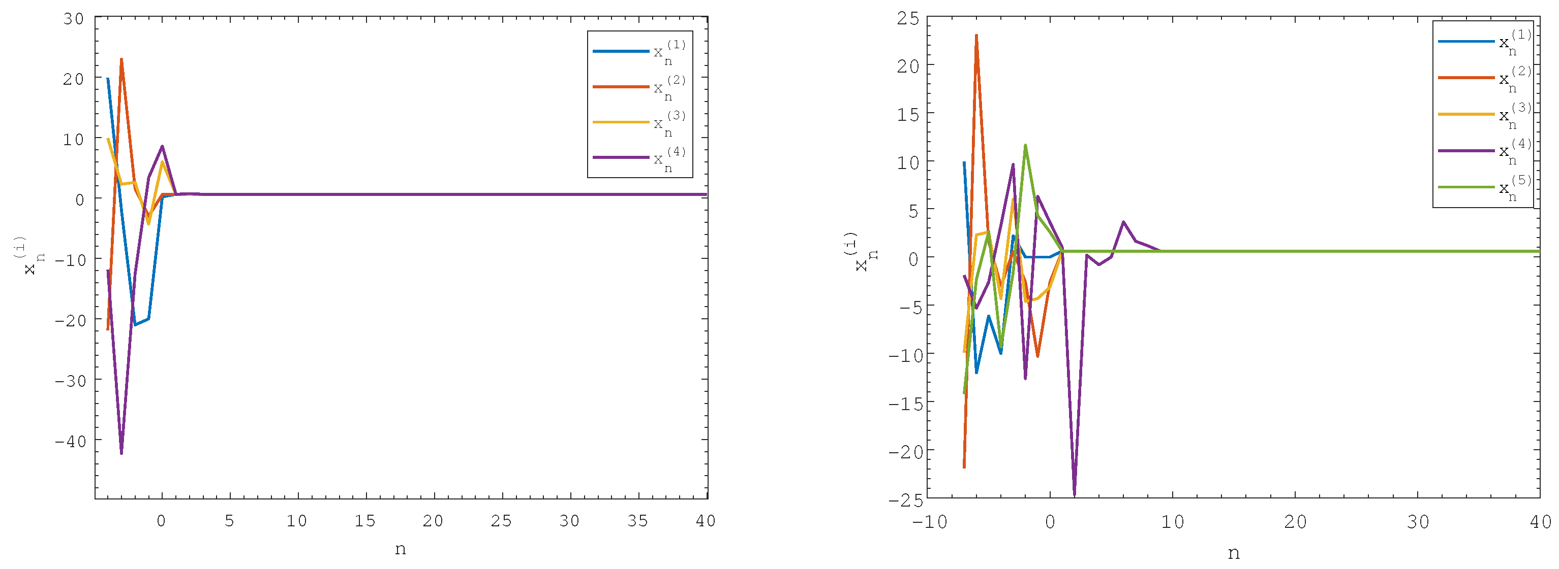
5. Numerical Examples

Example 7.

Consider system (3) with $m=3,k=4$ and $\theta =4$. i.e., the system of difference equations

$$\begin{array}{c}{\displaystyle x_{n+1}^{\left(1\right)}=\frac{11+7x_{n-4}^{\left(2\right)}}{18+11x_{n-4}^{\left(2\right)}},x_{n+1}^{\left(2\right)}=\frac{11+7x_{n-4}^{\left(3\right)}}{18+11x_{n-4}^{\left(3\right)}},}\hfill \\ {\displaystyle x_{n+1}^{\left(3\right)}=\frac{11+7x_{n-4}^{\left(4\right)}}{18+11x_{n-4}^{\left(4\right)}},x_{n+1}^{\left(4\right)}=\frac{11+7x_{n-4}^{\left(1\right)}}{18+11x_{n-4}^{\left(1\right)}},}\hfill \end{array}n\in {\mathbb{N}}_0.$$

(15)

Figure 1 (left) represents system (15) with initial conditions $x_{-4}^{\left(1\right)}=19.9$, $x_{-3}^{\left(1\right)}=-2$, $x_{-2}^{\left(1\right)}=-21$, $x_{-1}^{\left(1\right)}=-20$, $x_0^{\left(1\right)}=0.2$, $x_{-4}^{\left(2\right)}=-21.9$, $x_{-3}^{\left(2\right)}=23$, $x_{-2}^{\left(2\right)}=1.6$, $x_{-1}^{\left(2\right)}=-3$, $x_{-0}^{\left(2\right)}=0.6$, $x_{-4}^{\left(3\right)}=9.9$, $x_{-3}^{\left(3\right)}=2.3$, $x_{-2}^{\left(3\right)}=2.6$, $x_{-1}^{\left(3\right)}=-4.3$, $x_0^{\left(3\right)}=6$, $x_{-4}^{\left(4\right)}=-11.9$, $x_{-3}^{\left(4\right)}=-42.3$, $x_{-2}^{\left(4\right)}=-12.7$, $x_{-1}^{\left(4\right)}=3.4$ and $x_0^{\left(4\right)}=8.6$

Example 7.

Consider system (3) with $m=6,k=7$ and $\theta =5$. i.e., the system of difference equations

$$\begin{array}{c}{\displaystyle x_{n+1}^{\left(1\right)}=\frac{47+29x_{n-7}^{\left(2\right)}}{76+47x_{n-7}^{\left(2\right)}},x_{n+1}^{\left(2\right)}=\frac{47+29x_{n-7}^{\left(3\right)}}{76+47x_{n-7}^{\left(3\right)}},x_{n+1}^{\left(3\right)}=\frac{47+29x_{n-7}^{\left(4\right)}}{76+47x_{n-7}^{\left(4\right)}},}\hfill \\ {\displaystyle x_{n+1}^{\left(4\right)}=\frac{47+29x_{n-7}^{\left(5\right)}}{76+47x_{n-7}^{\left(5\right)}},x_{n+1}^{\left(5\right)}=\frac{47+29x_{n-7}^{\left(1\right)}}{76+47x_{n-7}^{\left(1\right)}},n\in {\mathbb{N}}_0.}\hfill \end{array}$$

(16)

Figure 1 (right) represents system (16) with initial conditions $x_{-7}^{\left(1\right)}=9.9$, $x_{-6}^{\left(1\right)}=-12.0$, $x_{-5}^{\left(1\right)}=-11$, $x_{-4}^{\left(1\right)}=-10$, $x_{-3}^{\left(1\right)}=0.2$, $x_{-2}^{\left(1\right)}=-6.1$, $x_{-1}^{\left(1\right)}=-10$, $x_0^{\left(1\right)}=2.2$, $x_{-7}^{\left(2\right)}=-21.9$, $x_{-6}^{\left(2\right)}=23$, $x_{-5}^{\left(2\right)}=1.6$, $x_{-4}^{\left(2\right)}=-3$, $x_{-3}^{\left(2\right)}=0.6$, $x_{-2}^{\left(2\right)}=-2.6$, $x_{-1}^{\left(2\right)}=-10.3$, $x_{-0}^{\left(2\right)}=-2.6$ $x_{-7}^{\left(3\right)}=-9.9$, $x_{-6}^{\left(3\right)}=2.3$, $x_{-5}^{\left(3\right)}=2.6$, $x_{-4}^{\left(3\right)}=-4.3$, $x_{-3}^{\left(3\right)}=6$, $x_{-2}^{\left(3\right)}=-4.6$, $x_{-1}^{\left(3\right)}=-4.3$, $x_0^{\left(3\right)}=-3.12$, $x_{-7}^{\left(4\right)}=-1.9$, $x_{-6}^{\left(4\right)}=-5.3$, $x_{-5}^{\left(4\right)}=-2.6$, $x_{-4}^{\left(4\right)}=3.3$, $x_{-3}^{\left(4\right)}=9.6$, $x_{-2}^{\left(4\right)}=-12.6$, $x_{-1}^{\left(4\right)}=6.3$, $x_0^{\left(4\right)}=3.6$, $x_{-7}^{\left(5\right)}=-14.19$, $x_{-6}^{\left(5\right)}=-2.3$, $x_{-5}^{\left(5\right)}=2.6$, $x_{-4}^{\left(5\right)}=-9.3$, $x_{-3}^{\left(5\right)}=-1.6$, $x_{-2}^{\left(5\right)}=11.6$, $x_{-1}^{\left(5\right)}=4.3$ and $x_0^{\left(5\right)}=2.6$.

6. Conclusions

In this paper, we have derived the solutions to the system of difference equations

$$x_{n+1}^{\left(q\right)}={\displaystyle \frac{L_{m+2}+L_{m+1}{x}_{n-k}^{\left(\right(q+1)mod(\theta \left)\right)}}{L_{m+3}+L_{m+2}{x}_{n-k}^{\left(\right(q+1)mod(\theta \left)\right)}}},n\in {\mathbb{N}}_0,$$

where $k\in {\mathbb{N}}_0$, $m\in \mathbb{Z}$, $q=1,\cdots ,\theta$, $\theta \in \mathbb{N}$, and ${\left(L_n\right)}_{n=0}^{+\infty }$ is Lucas sequence.

The above-mentioned system is a more general system to some systems studied recently. The well-defined solutions to that system are represented in terms of Fibonacci and Lucas sequences.

Those well-defined solutions depend on whether $\theta$ is even or odd. When $\theta$ is even, we invoked the solution of the difference equation

$$u_{n+1}={\displaystyle \frac{F_{\theta (m+2)}+F_{\theta (m+2)-1}{u}_{n-(\theta -1)}}{F_{\theta (m+2)+1}+F_{\theta (m+2)}{u}_{n-(\theta -1)}}},n\in {\mathbb{N}}_0,$$

that was used in [26].

For odd values of $\theta$, we invoked the solution of the difference equation

$${\mathsf{\Omega }}_{n+1}={\displaystyle \frac{L_{\theta (m+2)}+L_{\theta (m+2)-1}{\mathsf{\Omega }}_n}{L_{\theta (m+2)+1}+L_{\theta (m+2)}{\mathsf{\Omega }}_n}},n\in {\mathbb{N}}_0.$$

The solution to that equation was derived in Appendix A.

System (3) has $2^{\theta }$ fixed points; one of these fixed points is locally asymptotically stable. Moreover, we proved that it is globally asymptotically stable.

References

1. Alzabut, J.; Selvam, A.G.M.; Dhakshinamoorthy, V.; Mohammadi, H.; Rezapour, S. On chaos of discrete time fractional order host-immune-tumor cells interaction model. J. Appl. Math. Comput. 2022, 68, 4795–4820. [Google Scholar] [CrossRef]
2. Almatrafi, M.B.; Berkal, M. Bifurcation Analysis and Chaos Control for Prey-Predator Model with Allee Effect. Int. J. Anal. Appl. 2023, 21, 131. [Google Scholar] [CrossRef]
3. Berkal, M.; Navarro, J.F.; Almatrafi, M.B. Qualitative Behavior for a Discretized Conformable Fractional-Order Lotka-Volterra Model with Harvesting Effects. Int. J. Anal. Appl. 2024, 22, 51. [Google Scholar] [CrossRef]
4. Berkal, M.; Almatrafi, M.B. Bifurcation and Stability of Two-Dimensional Activator–Inhibitor Model with Fractional-Order Derivative. Fractal Fract. 2023, 7, 344. [Google Scholar] [CrossRef]
5. Berkal, M.; Navarro, J.F. Qualitative behavior of a two-dimensional discrete-time prey–predator model. Comput. Math. Methods 2021, 3, e1193. [Google Scholar] [CrossRef]
6. Koshy, T. Fibonacci and Lucas Numbers with Applications; Wiley: Hoboken, NJ, USA, 2001. [Google Scholar]
7. Abo-Zeid, R. Forbidden sets and stability in some rational difference equations. J. Differ. Equ. Appl. 2018, 24, 220–239. [Google Scholar] [CrossRef]
8. Abo-Zeid, R. Global behavior of two third order rational difference equations with quadratic terms. Math. Slovaca 2019, 69, 147–158. [Google Scholar] [CrossRef]
9. Abo-Zeid, R. Global behavior of a fourth-order difference equation with quadratic term. Bol. Soc. Mat. Mex. 2019, 25, 187–194. [Google Scholar] [CrossRef]
10. Abo-Zeid, R. Behavior of solutions of a rational third order difference equation. J. Appl. Math. Inform. 2020, 38, 1–12. [Google Scholar]
11. Abo-Zeid, R. On the solutions of a higher order recursive sequence. Malaya J. Mat. 2020, 8, 695–701. [Google Scholar] [CrossRef]
12. Atpinar, S.; Yazlik, Y. Qualitative behavior of exponential type of fuzzy difference equations system. J. Appl. Math. Comput. 2023, 69, 4135–4162. [Google Scholar] [CrossRef]
13. Berkal, M.; Navarro, J.F. Qualitative study of a second order difference equation. Turk. J. Math. 2023, 47, 516–527. [Google Scholar] [CrossRef]
14. Berkal, M.; Berehal, K.; Rezaiki, N. Representation of solutions of a system of five-order nonlinear difference equations. J. Appl. Math. Inform. 2022, 40, 409–431. [Google Scholar]
15. Gümüş, M.; Abo-Zeid, R. An explicit formula and forbidden set for a higher order difference equation. J. Appl. Math. Comput. 2020, 63, 133–142. [Google Scholar] [CrossRef]
16. Gümüş, M.; Abo-Zeid, R. Global behavior of a rational second order difference equation. J. Appl. Math. Comput. 2020, 62, 119–133. [Google Scholar] [CrossRef]
17. Ghezal, A. Note on a rational system of (4k+1)-order difference equations: Periodic solution and convergence. J. Appl. Math. Comput. 2023, 69, 2207–2215. [Google Scholar] [CrossRef]
18. Ghezal, A.; Balegh, M.; Zemmouri, I. Solutions and local stability of the Jacobsthal system of difference equations. AIMS Math. 2024, 9, 3576–3591. [Google Scholar] [CrossRef]
19. Haddad, N.; Touafek, N.; Rabago, J.F.T. Well-defined solutions of a system of difference equations. J. Appl. Math. Comput. 2018, 56, 439–458. [Google Scholar] [CrossRef]
20. Halim, Y.; Berkal, M.; Khelifa, A. On a three-dimensional solvable system of difference equations. Turk. J. Math. 2020, 44, 1263–1288. [Google Scholar] [CrossRef]
21. Halim, Y.; Khelifa, A.; Berkal, M. Representation of solutions of a two-dimensional system of difference equations. Miskolc Math. Notes 2020, 21, 203–218. [Google Scholar] [CrossRef]
22. Halim, Y.; Khelifa, A.; Berkal, M.; Bouchair, A. On a solvable system of p difference equations of higher order. Period. Math. Hung. 2022, 85, 109–127. [Google Scholar] [CrossRef]
23. Hamioud, H.; Touafek, N.; Dekkar, I.; Yazlik, Y. On a three dimensional nonautonomous system of difference equations. J. Appl. Math. Comput. 2022, 68, 3901–3936. [Google Scholar] [CrossRef]
24. Khelifa, A.; Halim, Y.; Berkal, M. Solutions of a system of two higher-order difference equations in terms of Lucas sequence. Univers. J. Math. Appl. 2019, 2, 202–211. [Google Scholar]
25. Khelifa, A.; Halim, Y.; Bouchair, A.; Berkal, M. On a system of three difference equations of higher order solved in terms of Lucas and Fibonacci numbers. Math. Slovaca 2020, 70, 641–656. [Google Scholar] [CrossRef]
26. Khelifa, A.; Halim, Y. General solutions to systems of difference equations and some of their representations. J. Appl. Math. Comput. 2021, 67, 439–453. [Google Scholar] [CrossRef]
27. Khelifa, A.; Halim, Y.; Berkal, M. On the solutions of a system of (2p+1) difference equations of higher order. Miskolc Math. Notes 2021, 22, 331–350. [Google Scholar] [CrossRef]
28. Kara, M. Investigation of the global dynamics of two exponential-form difference equations systems. Electron. Res. Arch. 2023, 31, 6697–6724. [Google Scholar] [CrossRef]
29. Kara, M.; Yazlik, Y. Solvable three-dimensional system of higher-order nonlinear difference equations. Filomat 2022, 36, 3449–3469. [Google Scholar] [CrossRef]
30. Stevic, S. Representation of solutions of bilinear difference equations in terms of generalized Fibonacci sequences. Electron. J. Qual. Theory Differ. Equ. 2014, 2014, 1–15. [Google Scholar] [CrossRef]
31. Stević, S.; Iričanin, B.; Kosmala, W.; Šmarda, Z. Note on the bilinear difference equation with a delay. Math. Methods Appl. Sci. 2018, 41, 9349–9360. [Google Scholar] [CrossRef]
32. Tollu, D.T.; Yazlik, Y.; Taskara, N. On the solutions of two special types of Riccati difference equation via Fibonacci numbers. Adv. Differ. Equ. 2013, 2013, 1–7. [Google Scholar] [CrossRef]
33. Berkal, M.; Abo-Zeid, R. Solvability of a Second-Order Rational System of Difference Equations. Fundam. J. Math. Appl. 2023, 6, 232–242. [Google Scholar] [CrossRef]
34. Kara, M.; Yazlik, Y. On eight solvable systems of difference equations in terms of generalized Padovan sequences. Miskolc Math. Notes 2021, 22, 695–708. [Google Scholar] [CrossRef]
35. Kara, M.; Yazlik, Y. Representation of solutions of eight systems of difference equations via generalized Padovan sequences. Internat. J. Nonlinear Anal. Appl. 2021, 12, 447–471. [Google Scholar]
36. Yazlik, Y.; Tollu, D.T.; Taskara, N. On the solutions of difference equation systems with Padovan numbers. Appl. Math. 2013, 4, 15. [Google Scholar] [CrossRef]
37. Vajda, S. Fibonacci and Lucas Numbers, and the Golden Section: Theory and Applications; Courier Corporation: New York, NY, USA, 2008. [Google Scholar]
Figure 1. A graph representing the global stability of system (15) (left) and system (16) (right).
Mca 29 00028 g001
Disclaimer/Publisher’s Note: The statements, opinions and data contained in all publications are solely those of the individual author(s) and contributor(s) and not of MDPI and/or the editor(s). MDPI and/or the editor(s) disclaim responsibility for any injury to people or property resulting from any ideas, methods, instructions or products referred to in the content.