A Rapid and Convenient Procedure to Evaluate Optical Performance of Intraocular Lenses

Abstract

A new portable lens scanner was developed and tested for measuring focal lengths and relative contrast transfer of mono- and multifocal intraocular lenses (IOLs). A photograph of a natural scene was imaged in white light through an IOL in a water-filled cuvette, with their +21D base power largely neutralized by a −20D trial lens, using a USB monochrome video camera that could be focused via a laptop-controlled stepping motor from −8.5 to + 8.0D. The output of 10000 ON-OFF antagonistic “receptive fields” measuring the video image with adjustable diameter was continuously recorded by custom written software to quantify focus and relative contrast. Six monofocal and four multifocal IOLs, as well as two radial refractive gradient (RRG) lenses were measured. After calibration with trial lenses the optical powers and relative contrast transfer of mono- and multifocal IOLs were readily measured. Refractive power profiles measured in RRG lenses closely matched data obtained from the manufacturer. The lens scanner uses a rapidly operating procedure, is portable and can be used to verify positions of the focal planes of mono- and multifocal IOLs in less than 3 s.

1. Introduction

A variety of optical designs of intraocular lenses (IOL) is available to restore retinal image quality after cataract extraction. Lenses may be spherical (including spherical aberrations), aspherical (correcting spherical aberrations), diffractive (maximizing contrast by interference in the focal plane) or refractive (standard non-coherent optical imaging). Furthermore, rather than focusing at a single plane, lenses may be multifocal (mostly bifocal) to add a secondary focal plane at the reading distance. Accordingly, image contrast is divided into different planes and has therefore lower values than with a monofocal IOL. Finally, efforts were made to develop IOL with extended depth of focus to permit reading without accommodation at a variety of distances [1]. It is clear that the extended depth of focus design is at the cost of image contrast. It is a matter of psychophysical studies to find out how much drop in image contrast is acceptable for the patient.

While the optical performance of an IOL can be calculated from the details of its optical design, direct measurements may be tedious and only a few instruments are available to measure multifocality. Among the first, Kusel and Rassow [2] implanted IOLs “optically” by using a telescope with a 1:1 magnification, in which one of the equally powered two lenses of the telescope were the IOLs, and tested contrast sensitivity functions psychophysically in human subjects. Later, many studies were done in which the image quality of IOLs was objectively measured. Such measurements are regulated by the International Standards Office (ISO), standard ISO 11979-2 for monofocal lenses and ISO 11979-9 for multifocal lenses. IOLs have to be placed into an industry standard Liou and Brennan eye model (Liou and Brennan 1997) with a 5 mm artificial pupil. Image quality is measured at a wavelength of 550 nm. Such approaches were used, for instance, by Terwee et al [3] and Maxwell et al [4]. These authors measured the optical performance of IOLs by analyzing the sharpness and contrast in the image generated from the United State Air Force 1951 Resolution target. The ISO eye model may however not be appropriate for all types of IOLs. For instance, it was recognized that it may not be valid for assessing aspherical lenses [5]. According to ISO 11979-2, a tolerance in refractive power of IOLs of up to +0.5D is acceptable. Therefore, a new measurement technique has to resolve at least half of diopter difference in IOL power. Moreover, since bifocal IOLs have the position of their secondary focal plane defined to precision of a quarter of a diopter, differences of this magnitude need to be resolved.

We have developed a novel procedure to measure refractive power of mono- and multifocal intraocular lenses in isolation (i.e., not in combination with a cornea model of an artificial eye). The technique involves automated video image analysis at 62 Hz video frame rate. It provides information on the relative contrast transfer at different spatial frequencies. It is fast and objective and takes less than 3 s to present a through-focus contrast curve from −8.5 to +8.0D at adjustable spatial frequencies.

2. Methods

2.1. Lenses

The following 6 monofocal lenses and 4 multifocal lenses artificial intraocular lenses were selected for measurements, based on their availability (Table 1A,B). ACRI.TEC 44S +21.0D was used during calibration, in combination with a −20D lens and further trial lenses (for details see below, “Calibration of the system”). In addition, two radial refractive gradient (RRG) lenses, custom-made by Rodenstock GmBH (Munich, Germany), as described by Tepelus et al. [6], were also measured.

Table 1. List of the intraocular lenses (IOLs) used in the current study. (A) Monofocal lenses; (B) Multifocal lenses.

(A)

Lens name, manufacturer	ACRI.TEC 44S, Surgicon Healthcare	TECNIS ASPHERIS ZCB00, Abbott Medical Optics	CT SPHERIS 204, Zeiss Meditec	CT ASPHERIS 509M, Zeiss Meditec	CT ASPHINA 509M, Zeiss Meditec	SN60WF, Alcon Pharma	DOMICRYL 677AB, Polytech-Domilens GmbH
Base power	+21.0D	+21.0D	+21.0D	+21.0D	+21.0D	+21.0D	+21.0D
Near add	none	none	none	none	none	none	None
Short name used in Figures	ACRITEC	TECNIS ASPH	SPHERIS	ASPHERIS	ASPHINA	ALCON +21	DOMILENS

(A)

Lens name, manufacturer	ACRI.TEC 44S, Surgicon Healthcare	TECNIS ASPHERIS ZCB00, Abbott Medical Optics	CT SPHERIS 204, Zeiss Meditec	CT ASPHERIS 509M, Zeiss Meditec	CT ASPHINA 509M, Zeiss Meditec	SN60WF, Alcon Pharma	DOMICRYL 677AB, Polytech-Domilens GmbH
Base power	+21.0D	+21.0D	+21.0D	+21.0D	+21.0D	+21.0D	+21.0D
Near add	none	none	none	none	none	none	None
Short name used in Figures	ACRITEC	TECNIS ASPH	SPHERIS	ASPHERIS	ASPHINA	ALCON +21	DOMILENS

(B)

Lens name, manufacturer	AT LISA 809M, Zeiss Meditec	TECNIS ZMB00, Abbott Medical Optics	SN6AD3, Alcon Pharma	SN6AD1, Alcon Pharma
Base power	+21.0D	+21.0D	+21.0D	+21.0D
Near add	+3.75D	+4.00D	+4.0D	+3.0D
Short name used in Figures	LISA	TECNIS MULT	ALCON +21 +4	ALCON +21 +3

(B)

Lens name, manufacturer	AT LISA 809M, Zeiss Meditec	TECNIS ZMB00, Abbott Medical Optics	SN6AD3, Alcon Pharma	SN6AD1, Alcon Pharma
Base power	+21.0D	+21.0D	+21.0D	+21.0D
Near add	+3.75D	+4.00D	+4.0D	+3.0D
Short name used in Figures	LISA	TECNIS MULT	ALCON +21 +4	ALCON +21 +3

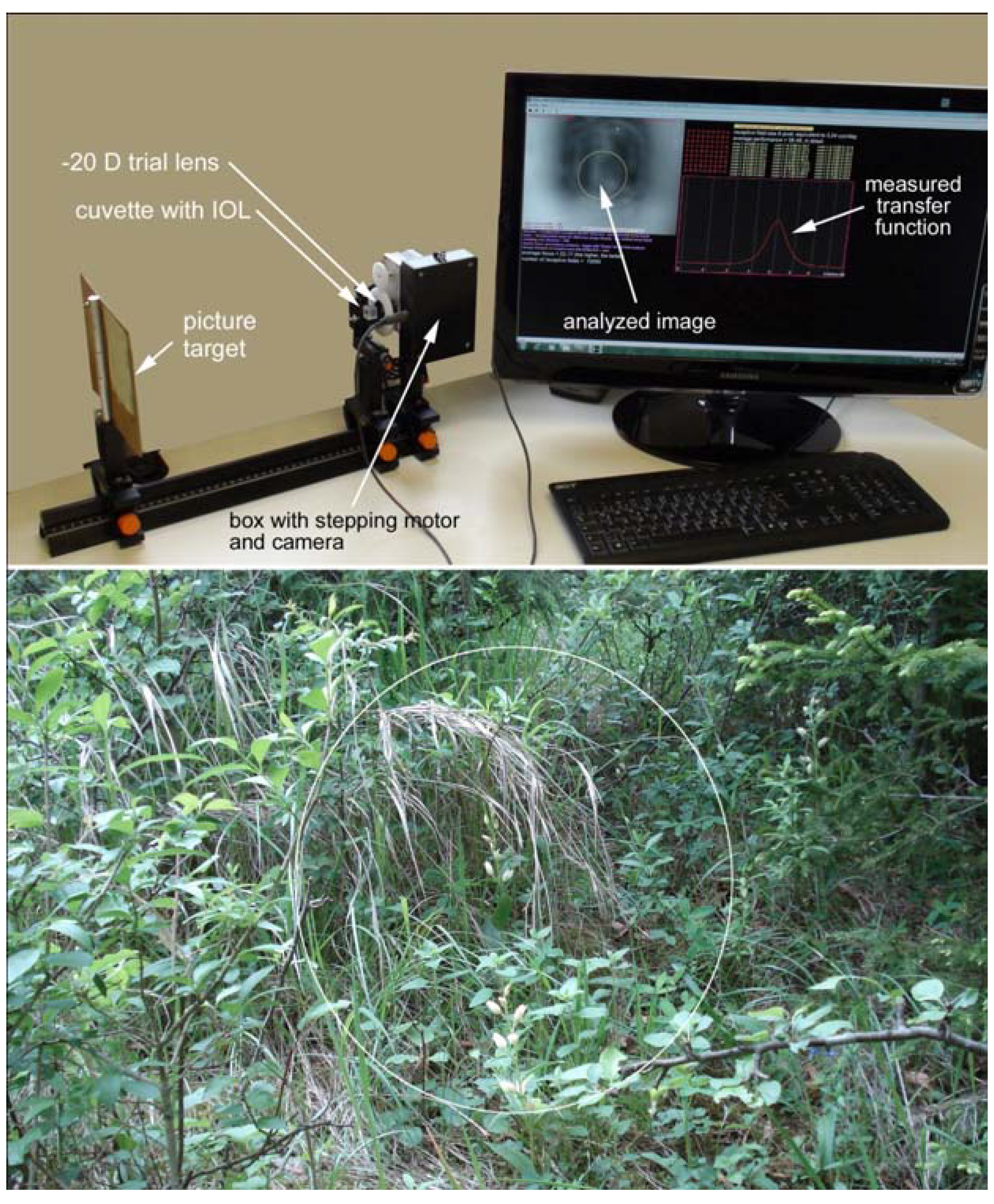
2.2. Hardware of the Lens Scanner

A monochrom-USB-Camera (DMK21AU04, TheImagingSource, Bremen, Germany) with a sampling rate of 62 Hz and a resolution of 640 × 480 Pixels was mounted on an optical track. It was equipped with a 8 mm, f/1.2 lens (TheImagingSource, Bremen, Germany). The camera imaged a printed photograph of a maddow scene (Figure 1B) that was presented at a distance of 18 cm (Figure 1A). Via a USB-controlled stepping motor, the camera was focused from −8.5 to +8.0 D in 150 individual steps in less than 3 s. The system was adjusted to provide the best focus between −0.5 and −1 D since the tested IOLs had a base power of +21 D but no −21 D trial lens was available for neutralization, but rather only −20 D.

Figure 1. (A) The lens scanner consisted of a monochrome video camera mounted on an optical track and equipped with a lens that could be focused with a stepping motor over a range of −8.5 to +8.0D, relative to a printed picture (“picture target”), presented at a distance of 18 cm. The IOL was placed in small water-filled cuvette. A −20D trial lens (“20 D trial lens”) largely neutralized the base power of the IOL in the cuvette. (B) appearance of the printed picture that was used as “picture target” for the measurements of the relative contrast transfer of the IOL. The encircled picture area was imaged through the IOL and the resulting image analyzed by custom-written software. The target picture was selected because it contains a wide range of spatial frequencies and fine details.

Figure 1. (A) The lens scanner consisted of a monochrome video camera mounted on an optical track and equipped with a lens that could be focused with a stepping motor over a range of −8.5 to +8.0D, relative to a printed picture (“picture target”), presented at a distance of 18 cm. The IOL was placed in small water-filled cuvette. A −20D trial lens (“20 D trial lens”) largely neutralized the base power of the IOL in the cuvette. (B) appearance of the printed picture that was used as “picture target” for the measurements of the relative contrast transfer of the IOL. The encircled picture area was imaged through the IOL and the resulting image analyzed by custom-written software. The target picture was selected because it contains a wide range of spatial frequencies and fine details.

IOLs were placed in a small quarz cuvette (1 × 1 × 1 cm) that was filled with distilled water to prevent salt deposits. The optical effect of distilled water (n = 1.333) versus vitreous of a real eye (n = 1.335) is less than 1%, or about 0.2 diopters at a refractive power of 21 D. The IOL was stabilized in the cuvette by a custom-made plastic holder. An artificial pupil limited the aperture size (see “cuvette with IOL”, Figure 1A). A 5 mm “pupil size” was chosen in accordance with many previous studies (i.e., [4,7]).

The picture target was illuminated by “room light” (combination of day light through the window and incandescent white light from the ceiling, with a luminance of about 50 cd/m²) and the average pixel brightness of the image of the target was constant throughout the measurements.

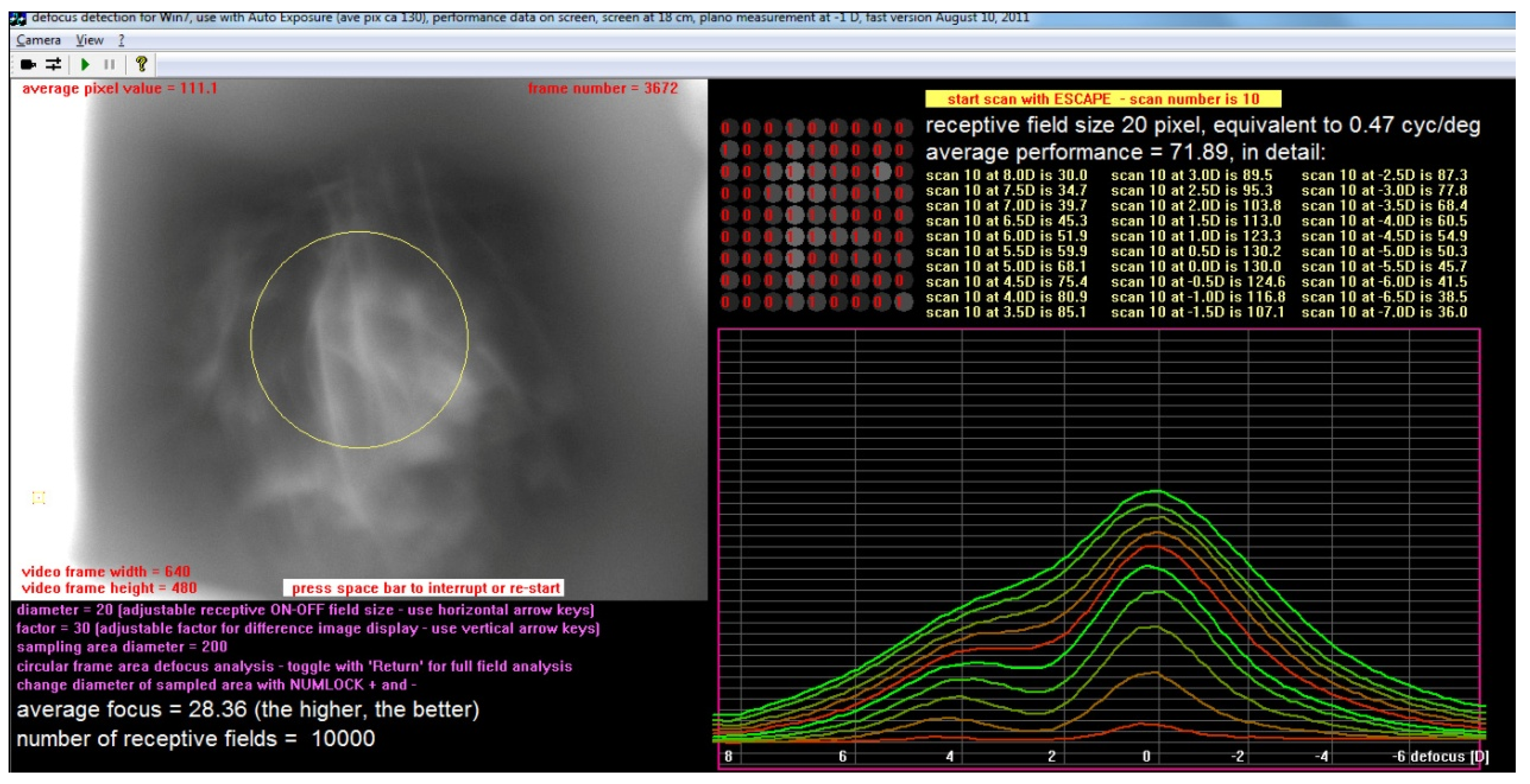
2.3. Image Processing and Software

Software was written in Visual C++ 8.0 to measure the average relative image contrast as a function of spatial frequency. Rather than using Fourier analysis to determine the contrast at a given spatial frequency, a circular image area (denoted by a yellow line in Figure 2) was sampled with “receptive fields”, similar to the ones in the retina. The output of a receptive field was defined as the absolute difference between the pixel brightness in the center and the averaged pixel brightness of the four pixels at the edges of a square, centered on the central pixel. The output of the receptive fields was summed up across the video frame in two pixel distance steps (n = 10,000). The sum was displayed on the screen and was taken as a measure of the average contrast of the video image. The diagonal diameter of the squared receptive field was considered equivalent to one spatial wavelength. Spatial frequency (in cyc/deg) was determined as the reciprocal of the angular diagonal diameter of the receptive field. It is important to realize that the spatial frequency range that could be evaluated was finally limited by pixel size in the video image. The smallest possible receptive field diameter (and accordingly the smallest wavelength that could be evaluated) was two pixels * sqrt(2). Accordingly, the highest measurable spatial frequency was 1/(2 pixel*sqrt(2)), which converts into 4.65 cyc/deg. While it is clear that this spatial frequency is far below the limits of human visual acuity (>30 cyc/deg), the variables of interest could be determined even when the low spatial frequency band below 4.65 cyc/deg was used: the positions of the two focal planes became already clearly visible when the spatial frequency was above 1 cyc/deg (Figure 2). For lower spatial frequencies, the depth of focus increased so that the two peaks were no longer resolved (Figure 2, uppermost curve).

The procedure is performed in “real-time”, e.g., relative contrast transfer is measured at the frame rate of the video camera (62 Hertz) and continuously displayed on the screen (Figure 2), and is denoted as “average focus”, in the bottom left.

The stepping motor could be activated from the key board and moved the camera lens once through the full range of focus. At the same time, the average relative contrast for each focus position was plotted as a continuous line on the screen (Figure 2, bottom right). The user could chose different receptive field sizes by the arrow keys. Data from a sample sequence of spatial frequencies ranging from 4.65 to 0.47 cyc/deg is shown in Figure 2. At best focus, the sum of the absolute outputs of all the receptive fields reached a peak. Data, representing the average contrast versus dioptric amount of defocus, were exported in ASCII format which can be exported into conventional data analysis programs like Windows Microsoft Excel.

Figure 2. “Screenshot” of the software output during the measurement of a sample bifocal IOL (LISA, with a base power of +21 D and a second focus at +3.75 D). The different curves on the right represent the summed output of the “receptive fields” (denoted as “average focus” on the bottom left) at different spatial frequencies. The lowest curve is the output at 4.65 cyc/deg, the highest at 0.47 cyc/deg. Note that the poor focus of the test image (see Figure 2B) is not due to inaccuracies in the system but rather because it was defocused by 8D when the screen shot was taken.

Figure 2. “Screenshot” of the software output during the measurement of a sample bifocal IOL (LISA, with a base power of +21 D and a second focus at +3.75 D). The different curves on the right represent the summed output of the “receptive fields” (denoted as “average focus” on the bottom left) at different spatial frequencies. The lowest curve is the output at 4.65 cyc/deg, the highest at 0.47 cyc/deg. Note that the poor focus of the test image (see Figure 2B) is not due to inaccuracies in the system but rather because it was defocused by 8D when the screen shot was taken.

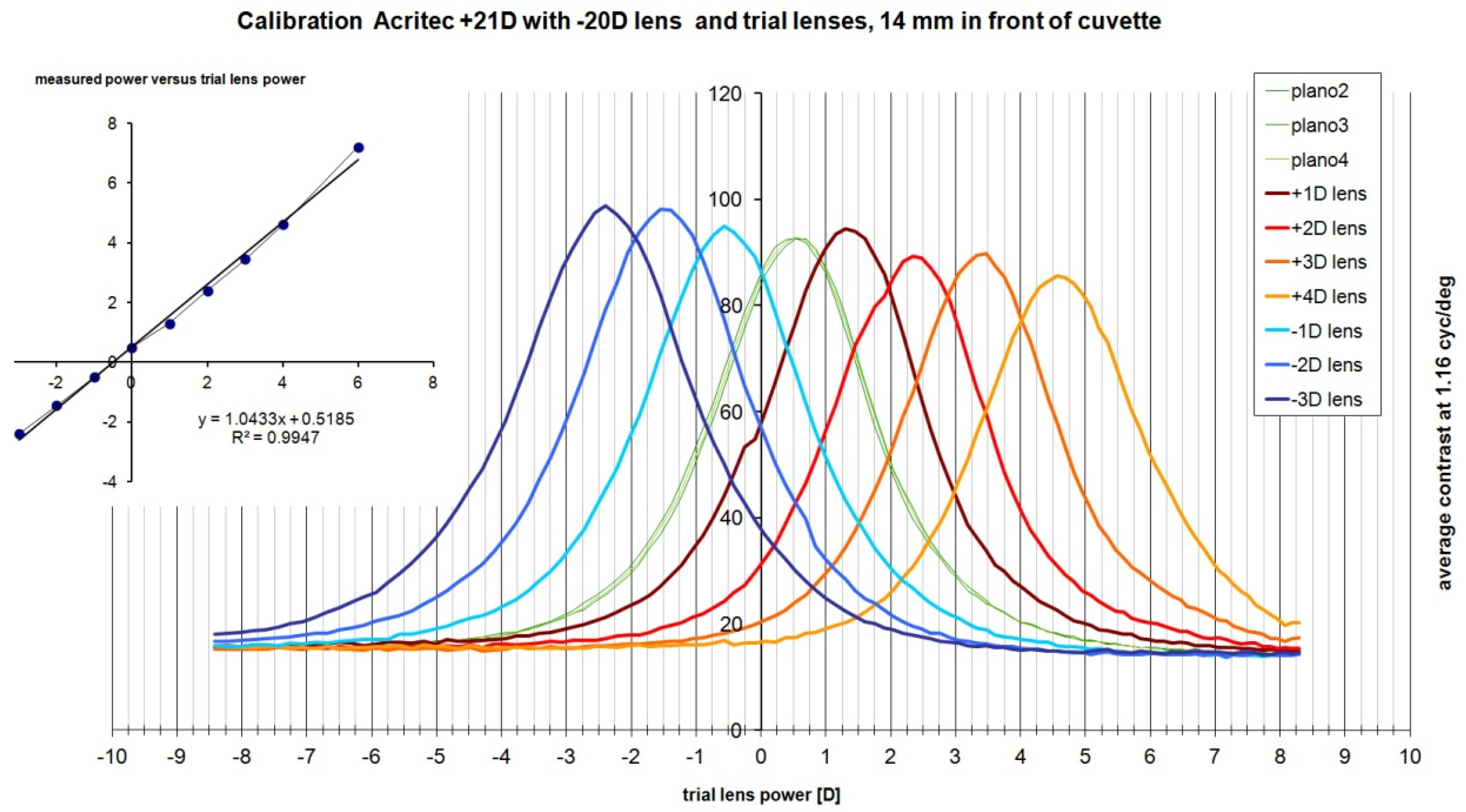
2.4. Calibration of the System

For calibration, standard trial lenses were held in front of the cuvette which contained a ACRITEC +21.0 D IOL and a −20D trial lens between cuvette and camera to neutralize the power of the IOL (Figure 1A). The lenses shifted the peaks of the relative contrast transfer curves by defined amounts as shown in Figure 3. Plotting peak positions of the curves versus trial lens power showed that a regression (inset in the top left in Figure 3) had a slope of almost one, with a correlation coefficient of close to one, indicating a highly linear relationship between the measured and the true lens powers. The small offset of 0.51 D suggests that the measured IOLs may have been about half a diopter less powerful than shown in the figures below. Figure 3 also demonstrates that the power of trial lenses (or spectacle lenses) could be readily determined from a single scan.

The peak height decreased slightly with increasing positive power of the trial lens (Figure 3). This effect could have been corrected by a linear operation but this was not done in the current study. The effect was about 15% reduction in peak height over a range of 8 D (Figure 3).

It remains to be determined how the summed output of the “receptive fields” can provide information about the absolute contrast transfer of the tested lenses at different spatial frequencies and different amounts of defocus. It is clear that measurements of absolute contrast requires that the pixel into luminance conversion of the video system is known (CCD chip, digital converter, potential automatic gain control by software which was however switched off). Second, contrast can only be determined relative to the maximal contrast that can be generated with no defocus present, which is determined by the response function of the video system and the optical quality of the camera lens. Even though basically possible, it was not attempted to do these corrections. Because absolute contrast was not measured, all contrast data refer to “relative contrast” with unknown conversion functions from real to measured contrast. Accordingly, the “relative contrast” data have no unit. Comparisons between different lenses and amounts of defocus should still be possible.

Figure 3. Calibration of the lens scanner with a set of trial lenses. Different trial lenses were held in front of the cuvette, containing a +21D ACRITEC monofocal lens, and a −20D trial between cuvette and camera. Depending on the spherical power of the trial lenses, the peaks of the transmission curves were shifted. The slope of a regression of peak position versus lens power was almost 1, indicating that the lens scanner was appropriately calibrated.

Figure 3. Calibration of the lens scanner with a set of trial lenses. Different trial lenses were held in front of the cuvette, containing a +21D ACRITEC monofocal lens, and a −20D trial between cuvette and camera. Depending on the spherical power of the trial lenses, the peaks of the transmission curves were shifted. The slope of a regression of peak position versus lens power was almost 1, indicating that the lens scanner was appropriately calibrated.

3. Results

A number of different IOLs were placed in the cuvette. Measurements for each lens were repeated three times, and IOLs were always removed from the cuvette and returned for the next measurement to be able to evaluate the variability introduced by repositioning the lenses. The three repetitions permitted to evaluate the effects of random variations in IOL positions in the cuvette which can be evaluated from the standard deviations shown in Figure 4 and Figure 5 (green curves).

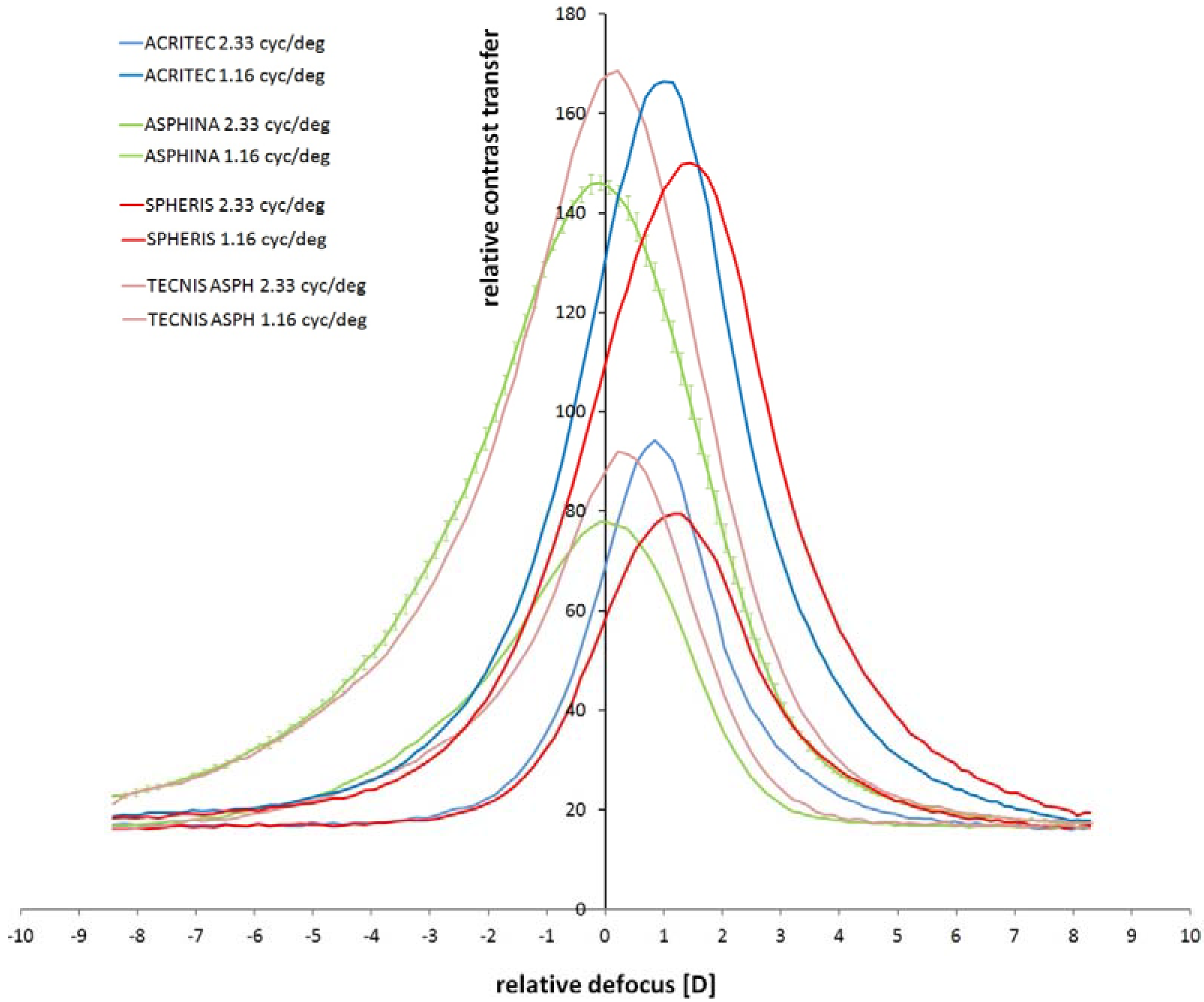
3.1. Measurement of Monofocal Lenses

Averages from three measurements of monofocal lenses are shown in Figure 4. Representative standard deviations are shown in one case for ASPHINA at 1.16 cyc/deg (green). Data were obtained for a wide range of spatial frequencies but only the data recorded at spatial frequencies of 2.33 cyc/deg and 1.16 cyc/deg are shown in Figure 4 for better clarity. The four tested monofocal IOLs did not differ much in their relative peak contrasts. The order of relative peak heights were similar at 1.16 cyc/deg (high peaks in Figure 4) and 2.33 cyc/deg (low peaks in Figure 4). It is interesting, however, that the peak positions for each IOL type were not always exactly between +0.5 D and +1.0 D as expected from the calibration when they had exactly 21.0 D base power (Figure 3) but varied around this value by about 1D. Possible reasons include variable centrations of the lenses in the cuvette, at least in those cases where their powers varied across their diameters. Peaks positions along the defocus axis were similar at both spatial frequencies for each lens.

Figure 4. Relative contrast in the images generated by four different monofocal IOLs at two different spatial frequencies (2.33 and 1.16 cyc/deg) as a function of defocus. Same colors in the upper curves (measured at 1.16 cyc/deg) and the lower curves (measured at 2.33 cyc/deg) denote the same IOLs. In one case, the standard deviations are shown from three repeated measurements (ASPHINA at 1.16 cyc/deg, green).

Figure 4. Relative contrast in the images generated by four different monofocal IOLs at two different spatial frequencies (2.33 and 1.16 cyc/deg) as a function of defocus. Same colors in the upper curves (measured at 1.16 cyc/deg) and the lower curves (measured at 2.33 cyc/deg) denote the same IOLs. In one case, the standard deviations are shown from three repeated measurements (ASPHINA at 1.16 cyc/deg, green).

3.2. Measurement of Multifocal Lenses

The two multifocal IOLs measured in the study had the same power for the far point but differed by their near “addition” which was 4.0 D in the case of the TECNIS Multifocal lens (Figure 5, green), and +3.75 D in the case of the LISA (Figure 5, red). This small difference was clearly resolved, both at 1.16 cyc/deg and 2.33 cyc/deg (Figure 5). Relative contrast transfer was generally lower with the multifocal lenses than with the monofocal lenses, as expected (compare peak heights in Figure 4 and Figure 5).

Figure 5. Relative contrast in the images generated by two multifocal IOLs at two different spatial frequencies (2.33 and 1.16 cyc/deg) as a function of defocus. Same colors in the upper curves (1.16 cyc/deg) and the lower curves (2.33 cyc/deg) denote the same IOL. In one case, standard deviations are shown as observed in three repeated measurements (TECNIS at 1.16 cyc/deg, green).

Figure 5. Relative contrast in the images generated by two multifocal IOLs at two different spatial frequencies (2.33 and 1.16 cyc/deg) as a function of defocus. Same colors in the upper curves (1.16 cyc/deg) and the lower curves (2.33 cyc/deg) denote the same IOL. In one case, standard deviations are shown as observed in three repeated measurements (TECNIS at 1.16 cyc/deg, green).

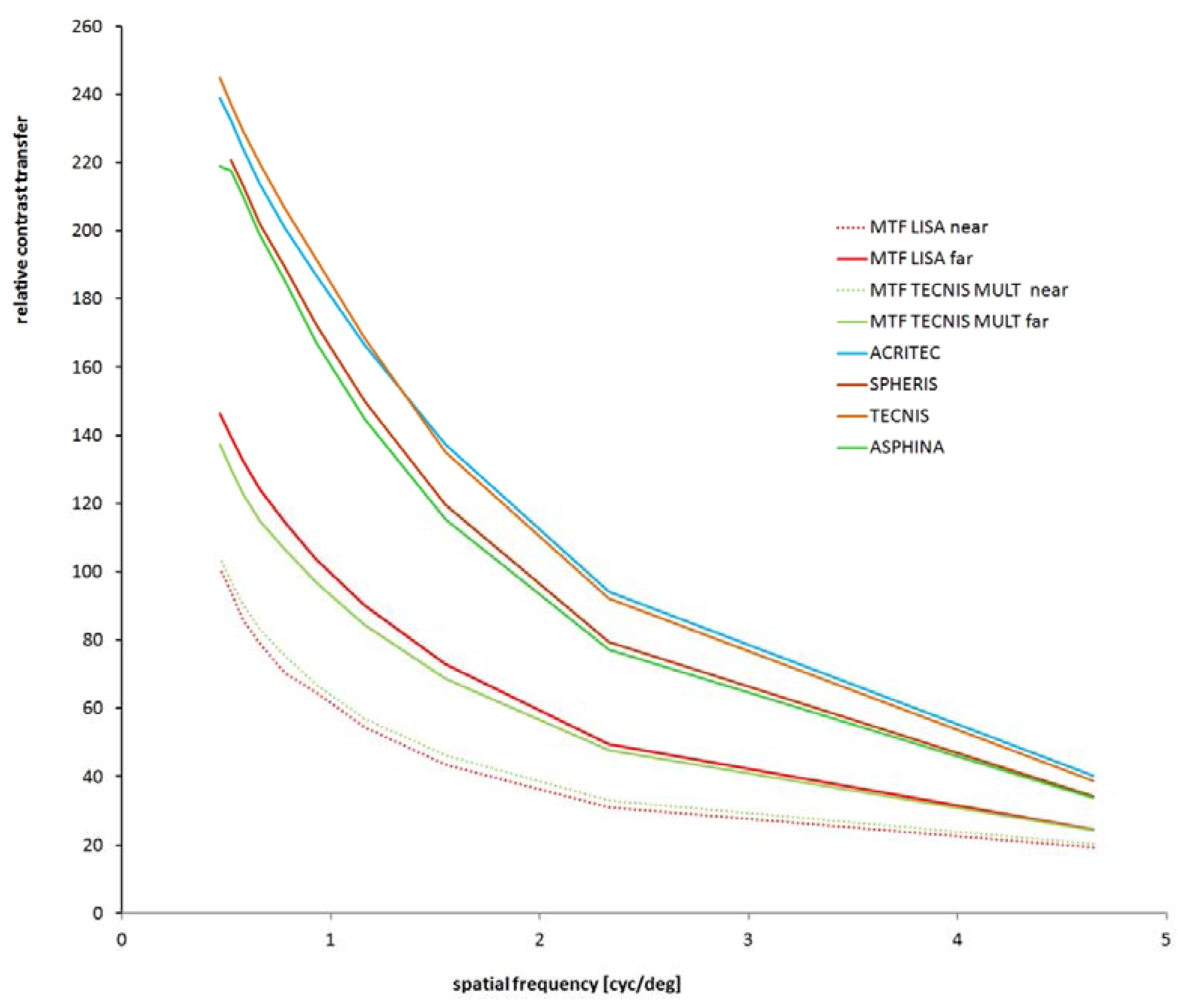
3.3. Relative Contrast Transfer at Different Spatial Frequencies

Next, the maximally achieved heights of the peaks, reflecting the contrast transfer of the lenses, were plotted against spatial frequency. As expected, contrast was highest at low spatial frequencies and declined continuously with increasing spatial frequency (Figure 6). Relative contrast transfer did not vary much between the four monofocal lenses, with the aspheric lens ASPINA slightly lower in contrast than the spheric lens SPHERIS. The multifocal lenses (red and green) were lower than the monofocal lenses, but both with better relative contrast at the focal plane intended for far vision (red and green, continuous lines) than for near vision (dotted lines). Note that the system could only measure contrast transfer at up to 4.65 cyc/deg because the pixel size in the video image precluded analyses at higher spatial frequencies.

Figure 6. Relative contrast transfer at different spatial frequencies of two multifocal lenses (near and far plane) and the four monofocal lenses, all measured at their best focus. Note that multifocal lenses did not differ much from each other and had less relative contrast at their focal plane for near vision, compared to far vision.

Figure 6. Relative contrast transfer at different spatial frequencies of two multifocal lenses (near and far plane) and the four monofocal lenses, all measured at their best focus. Note that multifocal lenses did not differ much from each other and had less relative contrast at their focal plane for near vision, compared to far vision.

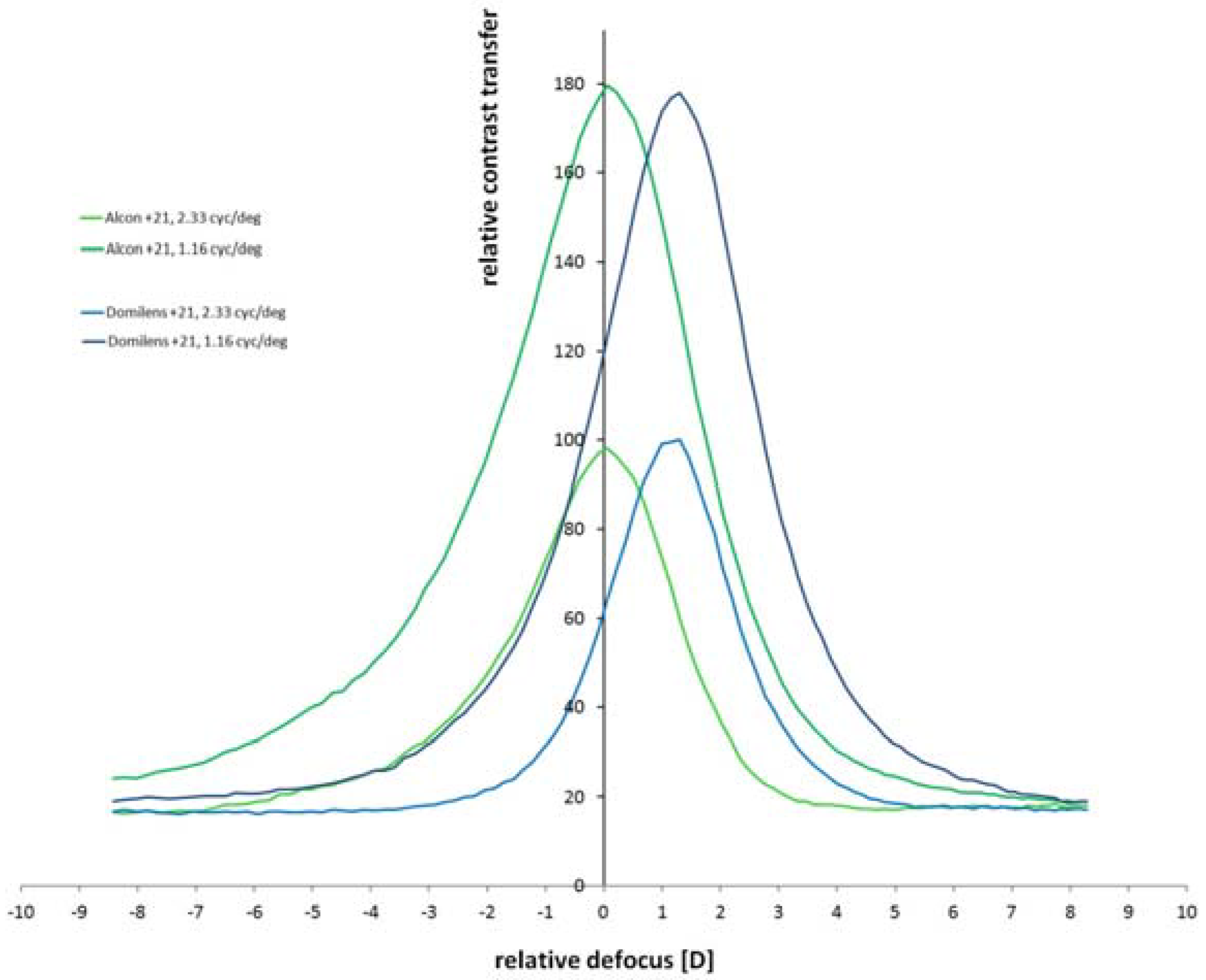
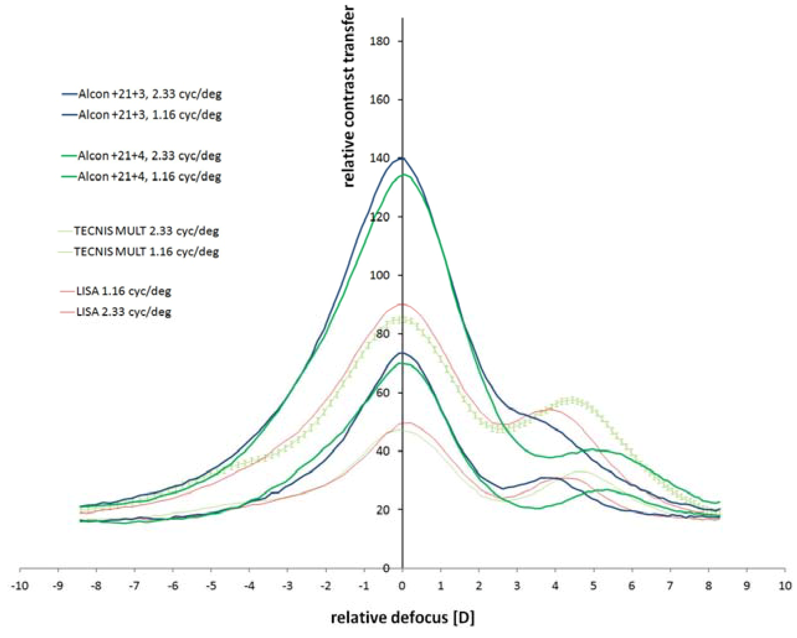
3.4. Measurements of Further Monofocal and Multifocal IOLs

To allow for comparisons, three additional lenses IOLs from ALCON with 21.0 D base power were also measured (one monofocal ALCON +21.0, two multifocal ALCON +21.0 with +4.0D and with +3.0D addition), as well as a monofocal DOMILENS with +21.0D power.

Relative contrast transfer at 2.33 cyc/deg and 1.16 cyc/deg were similar for the two monofocal lenses Alcon +21 and Domilens +21, but the Domilens had slightly more power in these measurements (Figure 7).

The different near additions in the two multifocal lenses Alcon +21 +3D and Alcon +21 +4D were readily resolved in the scans (Figure 8). These two lenses had much higher relative contrast transfer at the focal plane for distant vision than the LISA and TECHNIS MULT which were already measured and shown in Figure 5. The higher contrast at the far plane was, as expected, at the cost of the contrast in the focal plane for near vision. For comparison, data from these lenses are also shown in Figure 8.

Figure 7. Relative contrast transfer as a function of introduced defocus in two monofocal lenses (Alcon +21, green, and Domilens +21, blue) at 2.33 and 1.16 cyc/deg. The performance, as expressed in relative contrast transfer at the two spatial frequencies, in both lenses was very similar but the Domilens had more positive power in these measurements.

Figure 7. Relative contrast transfer as a function of introduced defocus in two monofocal lenses (Alcon +21, green, and Domilens +21, blue) at 2.33 and 1.16 cyc/deg. The performance, as expressed in relative contrast transfer at the two spatial frequencies, in both lenses was very similar but the Domilens had more positive power in these measurements.

Figure 8. Relative contrast transfer in two further multifocal lenses (Alcon +21D +3D, blue, and Alcon +21D +4D, green) at two different spatial frequencies. Relative contrast transfer of the two multifocal lenses, already shown in Figure 5, is also plotted as thin lines in the background for comparison. The differences in the optical power in the focal plane assigned to near vision (+3 versus +4D) are clearly resolved.

Figure 8. Relative contrast transfer in two further multifocal lenses (Alcon +21D +3D, blue, and Alcon +21D +4D, green) at two different spatial frequencies. Relative contrast transfer of the two multifocal lenses, already shown in Figure 5, is also plotted as thin lines in the background for comparison. The differences in the optical power in the focal plane assigned to near vision (+3 versus +4D) are clearly resolved.

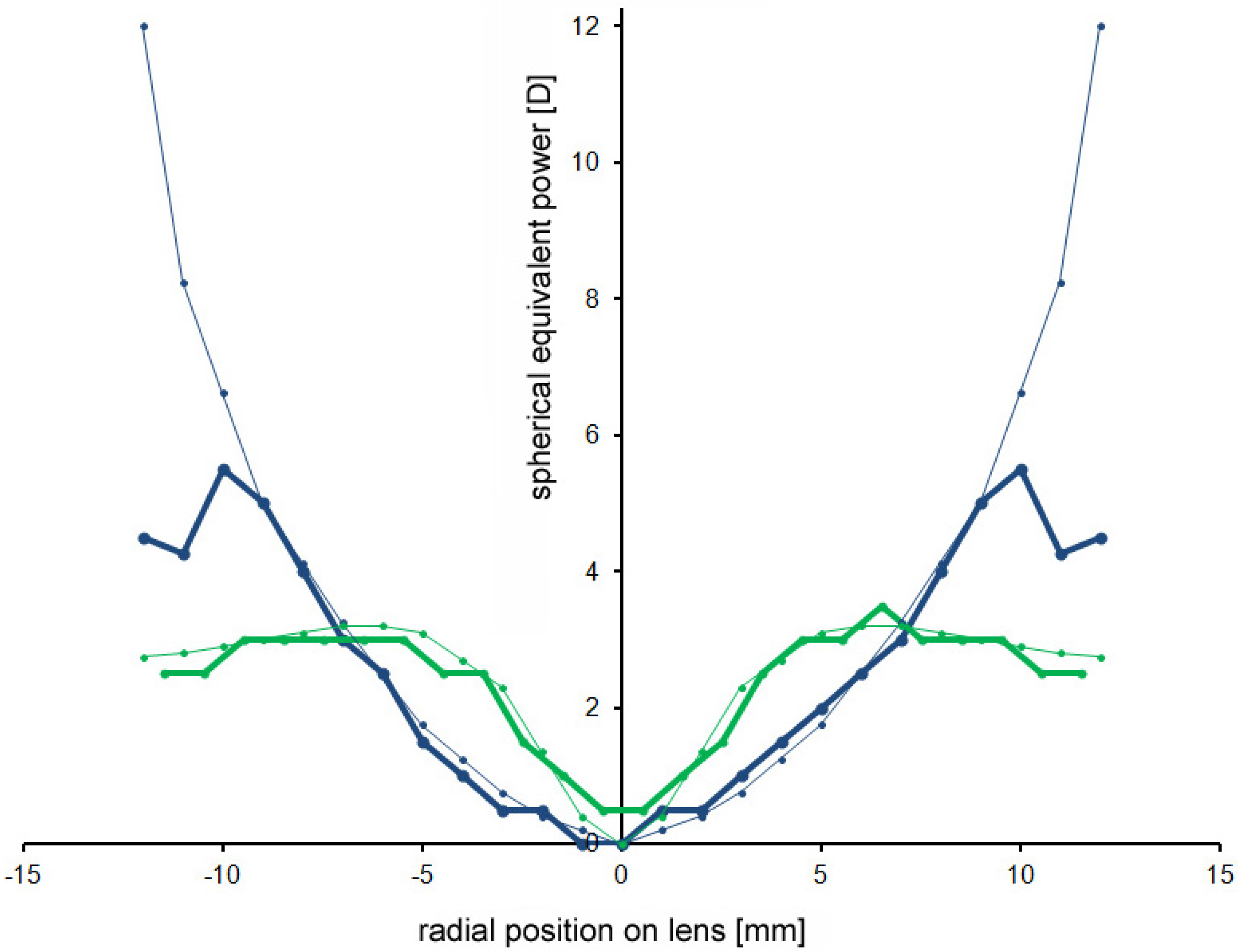
3.5. Measurement of Radial Refractive Gradient Lenses

The technique was also used to measure radial refractive gradient lenses (RRG). The two RRG lenses were designed by Rodenstock and used by Tepelus et al [6] for experiments in chickens. The spherical equivalent refractive power of the lenses at different distances from the lens center were available from the manufacturer (thin lines in Figure 9). To scan across the lens diameter, the lenses were placed on a micrometer-drive controlled linear track and moved laterally relative to the optical axis of the video camera. An artificial pupil with 1 mm diameter was inserted to be able to scan in 1 mm steps across the lens diameter. The peak positions of the scans along the diopter axis (as in Figure 2) were plotted against the radial position on the lens (Figure 9, thick lines). In both lens types, RRG1 and RRG2, a close agreement was found between measured lens power and the lens power provided by the manufacturer for rays parallel to the optical axis of the lens but at different radial eccentricities from the optical axis (Figure 9, thin lines). These findings show that the lens scanner could also be used to study the effects of centration of an IOL on contrast transfer and focal length.

Figure 9. Refractive power of two different refractive gradient lenses (RRG) lenses (green and blue) at different radial positions, as measured with the lens scanner (thick lines) and as provided by the manufacturer (thin lines). Both data sets show close agreement up to 10 mm off from the lens center. Beyond 10 mm, the system was limited by the mechanics of the cuvette holder.

Figure 9. Refractive power of two different refractive gradient lenses (RRG) lenses (green and blue) at different radial positions, as measured with the lens scanner (thick lines) and as provided by the manufacturer (thin lines). Both data sets show close agreement up to 10 mm off from the lens center. Beyond 10 mm, the system was limited by the mechanics of the cuvette holder.

4. Conclusions

The lens scanner was able to locate the dioptric positions of best focus of a lens and clearly resolved the dioptric positions of the secondary foci of multifocal lenses. The procedure was rapid (< 3 s) and intuitive since the relative contrast transfer function was plotted online on the computer screen for direct inspection. The transfer function could be determined at different spatial frequencies, which could be selected by the user. The procedure appears also useful to determine the depth of focus of the IOL, using defined criteria for the cut-off Strehl ratio [8].

A major question is: how well does the height of the relative contrast transfer function reflect the true contrast transfer function of the IOL? To ultimately resolve this question, detailed performance data of the lenses would be necessary, obtained from the manufacturer. At least, a few obvious differences were reproduced in the measurements: (1) the two multifocal lenses had lower relative contrast transfer at the plane for far vision than the monofocal lenses and (2) the contrast was lower at the near focus than at the far focus in all multifocal lenses (3) lenses that had more contrast at the focal plane for far vision had less contrast in the focal plane for near vision, as expected. It would be interesting to know whether the small differences in contrast transfer seen among the monofocal lenses (Figure 4) were also described by the lens manufacturers. The standard deviation of the lens scanner suggests that these difference were significant, despite that they were small.

4.1. Possible limitations of the Lens Scanner

Six limiting factors need consideration:

(1)

The positioning and centration of the IOL in the cuvette. The custom-made lens holder does not allow for perfect centration of the IOL in the camera axis since this was done manually with a pair of tweezers. In addition, it was found that even minor mechanical forces acting on the soft lenses caused a rapid decay of their optical performance.

(2)

Since both the “neutralizing” trial lens and IOL had high power, small differences in the axial positions of the lenses had severe effects on the measurements of their absolute optical power: 1 mm displacement was equivalent to about 0.6 D.

(3)

The linearity of the video camera. It is assumed that luminance differences between the receptive field center and periphery were converted into pixel differences, no matter what the absolute local brightness of the picture was. It is known that video systems show a more log-linear response which means brightness differences are not linearly encoded in pixel values. Related to this problem, saturation is not fully controlled. However, since the average contrast in the image is determined from the sum of the absolute outputs of 10,000 receptive fields at different places, these variations may partially average out. In the current set-up, the gain control of the video system was set on automatic, resulting in an average pixel brightness of the video image of about 130 in all cases.

(4)

The ISO standard 11979-2 requests that IOLs should have a modulation transfer at a pupil size of 3 mm of at least 0.43 at 100 cyc/mm, corresponding to about 34.5 cyc/deg on the retina (image magnification in the human eye: 290 µm/deg). The current set-up can only measure the modulation transfer at spatial frequencies up to 4.65 cyc/deg. To measure at 34.5 cyc/deg, as requested by ISO 11979-2, either a video camera needs to be used with much smaller pixels of the CCD chip, or the imaging lens needs to have a longer focal length.

(5)

The ISO standard 11979-2 requests IOL performance to be measured in monochromatic light of 550 nm. While it is clear that a defined wavelength has its merits, we believe that the broadband white light that was used in the current study matches the typical experience of the subjects. We expect that the refractive power differences that might be measured with our procedure in green light to be negligible. Moreover, it would be easy to illuminate the target (Figure 1) with monochromatic light by use of an interference filter.

(6)

The optical aberrations potentially introduced by the cuvette wall and the neutralizing lens were not studied. Potentially, both could introduce spherical aberration. However, a water or saline-filled cuvette was also used in previous studies to measure IOLs and other authors should have faced the same problem (i.e., [4]).

4.2. Comparison to Other Procedures to Measure the Performance of Artificial Intraocular Lenses

Previous approaches to measure the performance of IOLs include (1) direct imaging of through the tested lens and analysis of image quality [3] (2) analysis of the path of light rays passing through the lens [3,9] (3) measurement of wavefront aberrations after IOL implantation with a Hartmann-Shack wavefront sensor [10] or the double pass technique [11] (4) measurement of reading ability [12,13] (5) psychophysical measurements of contrast sensitivity and visual acuity when the IOL is “optically” implanted [2].

It is clear that psychophysical procedures describe visual performance most directly. Measurements of the optics of the eye after implantation are informative since they describe retinal image quality in vivo. To measure the optics of an IOL before implantation, not many options are available. Procedures (1) and (2) require a model eye (“average cornea eye” in [3] and elaborate analyses of the spatial frequency content of the recorded image, or the paths of light rays projected through the lenses. The procedure described in this paper does not require any calculations by the user: the relative contrast transfer at a given spatial frequency and the position of the best focus are immediately visible on the computer screen. Therefore, the advantages of the technique are that one can readily get accurate measurements of the power of any lens held in front of the scanner, and that this can be done at any position in the lens (if one is interested in refractive gradient lenses). Furthermore, multifocal lenses can be measured.

4.3. Outlook: Measurements of Absolute Contrast Transfer, Astigmatism, and at Higher Spatial Frequencies

While measurements of the dioptric positions of the focal planes of the measured IOL position are reproducible when the lens is always placed at the same axial position, measurements of the absolute contrast transfer may be affected by the linearity of the video system and should be further tested.

There are options to add additional features to the system like measurement of astigmatism. As can be expected, an astigmatic spectacle lens in front of the camera generates a broader contrast transfer curve in the lens scanner and also lower peak contrast. Using elliptic “receptive fields” with variable orientations, rather than squared receptive fields as used in the current software, astigmatic defocus and its axis could be immediately extracted from the image.

References

1. Zalevsky, Z. Extended depth of focus imaging: A review. SPIE Rev. 2010, 1, 018001. [Google Scholar]
2. Kusel, R.; Rassow, B. Preoperative assessment of intraocular lens corrected vision. Klin. Monbl. Augenheilkd. 1999, 215, 127–131. (In German) [Google Scholar] [CrossRef]
3. Terwee, T.; Weeber, H.; van der Mooren, M.; Piers, P. Visualization of the retinal image in an eye model with spherical and aspheric, diffractive, and refractive multifocal intraocular lenses. J. Refract. Surg. 2008, 24, 223–232. [Google Scholar]
4. Maxwell, W.A.; Lane, S.S.; Zhou, F. Performance of presbyopia-correcting intraocular lenses in distance optical bench tests. J. Cataract Refract. Surg. 2009, 35, 166–171. [Google Scholar] [CrossRef]
5. Norrby, S. ISO eye model not valid for assessing aspherical lenses. J. Cataract Refract. Surg. 2008, 34, 1056–1057. [Google Scholar] [CrossRef]
6. Tepelus, T.C.; Vazquez, D.; Seidemann, A.; Uttenweiler, D.; Schaeffel, F. Effects of lenses with different power profiles on eye shape in chickens. Vision Res. 2012, 54, 12–19. [Google Scholar] [CrossRef]
7. Kim, M.J.; Zheleznyak, L.; MacRae, S.; Tchah, H.; Yoon, G. Optical evaluation of through-focus optical performance of presbyopia-correcting intraocular lenses using an optical bench system. J. Cataract Refract. Surg. 2011, 37, 1305–1312. [Google Scholar] [CrossRef]
8. Marcos, S.; Barbero, S.; Jiménez-Alfaro, I. Optical quality and depth-of-field of eyes implanted with spherical and aspheric intraocular lenses. J. Refract. Surg. 2005, 21, 223–235. [Google Scholar]
9. Piers, P.A.; Weeber, H.A.; Artal, P.; Norrby, S. Theoretical comparison of aberration-correcting customized and aspheric intraocular lenses. J. Refract. Surg. 2007, 23, 374–384. [Google Scholar]
10. Bellucci, R.; Morselli, S.; Piers, P. Comparison of wavefront aberrations and optical quality of eyes implanted with five different intraocular lenses. J. Refract. Surg. 2004, 20, 297–306. [Google Scholar]
11. Navarro, R.; Ferro, M.; Artal, P.; Miranda, I. Modulation transfer functions of eyes implanted with intraocular lenses. Appl. Opt. 1993, 32, 6359–6367. [Google Scholar] [CrossRef]
12. Hütz, W.W.; Eckhardt, H.B.; Röhrig, B.; Grolmus, R. Reading ability with 3 multifocal intraocular lens models. J. Cataract Refract. Surg. 2006, 32, 2015–2021. [Google Scholar]
13. Richter-Mueksch, S.; Weghaupt, H.; Skorpik, C.; Velikay-Parel, M.; Radner, W. Reading performance with a refractive multifocal and a diffractive bifocal intraocular lens. J. Cataract Refract. Surg. 2002, 28, 1957–1963. [Google Scholar] [CrossRef]