Investigation of the Space-Variance Effect of Imaging Systems with Digital Holography
by
 and
and
Xingyu Yang
1, 
Rong Zhao
1,
Huan Chen
1,
Yijun Du
1,
Chen Fan
1,
Gaopeng Zhang
2 and
Zixin Zhao
1,* 1
State Key Laboratory for Manufacturing Systems Engineering, School of Mechanical Engineering, Xi’an Jiaotong University, Xi’an 710049, China
2
Xi’an Institute of Optics and Precision Mechanics, Chinese Academy of Sciences, Xi’an 710119, China
*
Author to whom correspondence should be addressed.
Photonics 2023, 10(12), 1350; https://doi.org/10.3390/photonics10121350
Submission received: 23 October 2023
/
Revised: 25 November 2023
/
Accepted: 30 November 2023
/
Published: 7 December 2023
(This article belongs to the Special Issue Optical Imaging and Measurements)
Abstract
:In classical Fourier optics, an optical imaging system is regarded as a linear space-invariant system, which is only an approximation. Especially in digital holography, the space-variance effect has a great impact on the image quality and cannot be ignored. Therefore, it is comprehensively investigated in this article. Theoretical analyses indicate that the space-variance effect is caused by linear frequency modulation and ideal low-pass filtering, and it can be divided into three states: the approximate space-invariance state, the high-frequency distortion state, and the boundary-diffraction state. Classical Fourier optics analysis of optical imaging systems only considers the first. Regarding the high-frequency distortion state, the closer the image field is to the edge, the more severe the distortion of high-frequency information is. As for the boundary-diffraction state, in addition to the distortion of high-frequency information in the margin, a prominent boundary-diffraction phenomenon is observed. If the space-variance effect of the imaging lens is ignored, we predict that no space-variance effect in image holography will occur when the hologram is recorded at the back focal plane of the imaging lens. Simulation and experimental results are presented to validate our theoretical prediction.
1. Introduction
In signal and systems theory, a system whose properties do not change with its spatial location is called a space-invariant system. In particular, the system response only depends on the input signal and the system characteristics and is independent of the spatial location where the input signal is imposed. Due to the linear space invariance of optical imaging systems, classical Fourier optics describes the optical imaging system in terms of the frequency response from the perspective of signals and systems [1].
However, the space invariance of optical imaging systems is only a simplification. Related studies have pointed out that the space variance lowers the image quality of the part of the image field that is farther away from the optical axis. Accordingly, this simplification may be inappropriate for some cases. Yan et al. [2] discussed the axial measurement error caused by the space-variance effect in digital holography by performing numerous simulations of point and line spread functions. Lohmann and Paris [3] defined the cross-correlation of two-line spread functions in an optical system as the evaluation index of the space-variance effect of the system. Moreover, Brainis [4] investigated the space-variance effect in aperture and lens imaging by analyzing the point spread function.
The aforementioned articles researched optical systems by analyzing the point spread function, which is classical in Fourier optics. The responses of any point or edge in a space-invariant system are the same, and every point or line is representative. A linear space-invariant system satisfies the convolution theorem, and its transfer function can be expressed by the Fourier transform of its point spread function. Therefore, point and edge spread functions can accurately describe the properties of space-invariant systems. However, no transfer function is present in the space-variant system, and the point spread function of a certain point can only describe the local response of the system to the point, which is unrepresentative. Therefore, it cannot holistically or comprehensively describe the system.
This study focuses on the causes of the space-variance effect, which have been studied by some scholars. Tichenor and Goodman [5] identified the quadratic phase factor as breaking the space-invariance condition of the single-lens imaging system. However, they only studied the conditions under which the quadratic phase factor can be ignored. Thus, although the optical imaging system can be simplified as a space-invariant system, the properties of the optical imaging system under space-variance effects cannot be analyzed. Pan et al. [6] showed that the spectrum broadening attributed to the quadratic phase factor was an important contribution to the space-variance effect, but their discussion on the space-variance effect was qualitative and not comprehensive. Herein, the role of the quadratic phase factor in the space-variance effect and its propagation law in digital holographic imaging systems are elucidated through a rigorous mathematical derivation.
Digital holography, an important three-dimensional measurement technology, can simultaneously record the intensity and phase information of the measured object. It is widely used in cell observation [7,8,9], particle and flow field measurement [10,11,12], and topography [13,14,15] and tomography [8,16,17] measurement, among others. According to the space-invariance approximation criterion proposed by Tichenor and Goodman [5], the width of the object field of view (FOV) should be less than 1/4 of the width of the aperture. This is easy to achieve for lens imaging. However, due to the limitation of the resolution and magnification in digital holography, the transverse size of the object under test or the virtual image of the front imaging system is usually comparable to the size of the CCD/CMOS chip, so the space-variance effect is very common in digital holography, especially digital Fresnel holography [18,19,20,21].
This paper analyzes the mathematical model of the Fresnel holographic imaging system and determines that the image field is not the result of the ideal low-pass filtering of the object field, as described in classical Fourier optics, but the result of the object field first modulated by the linear frequency modulation (LFM) signal and then filtered by the ideal low-pass filter. Thereafter, according to the ratio of the space–bandwidth product between the LFM signal and the aperture, the space-variance effect of the holographic imaging system is categorized into approximate space-invariance, high-frequency distortion, and boundary-diffraction states. Notably, the classical Fourier optical analysis of optical imaging systems only considers the approximate space-invariance state, which can be reduced to a space-invariant system. In the high-frequency distortion state, the closer the image field is to the FOV edge, the more severe the high-frequency information distortion is. In the boundary-diffraction state, in addition to the distortion of high-frequency information in the FOV margin, boundary-diffraction fringes are prominent. Specifically, the Fresnel diffraction pattern of the aperture stop can be observed in the image field. To validate our theory, we predict that no space-variance effect occurs in image holography [22,23] when the hologram is recorded in the back focal plane of the imaging lens if the space-variance effect of the imaging lens is ignored. Simulations and experiments were conducted to confirm this prediction. For simplicity, the theoretical derivation in this paper is based on the one-dimensional imaging case, but it can be easily extended to the two-dimensional case.
The rest of this article is organized as follows. In Section 2, the mathematical model of Fresnel holography considering the space-variance effect is established. In Section 3, the space-variance effect is divided into three states. In Section 4, the prediction is proposed and confirmed by the results of simulations and experiments.
2. Materials and Methods
2.1. Mathematical Model of Space-Variant Fresnel Holographic Imaging Systems
Diffraction in free space is linear space-invariant. According to the Huygens–Fresnel principle, “every unobstructed point of a wavefront, at a given instant, serves as a source of spherical quadratic wavelets. The amplitude of the optical field at any point beyond is the superposition of all these wavelets [24].”. The Huygens–Fresnel principle comprises two elements: the spherical wavelets hypothesis and the combination mode of spherical wavelets—interference superposition. If free-space diffraction is considered, the above points, respectively, correspond to the space-invariant and linear characteristics of free-space diffraction.
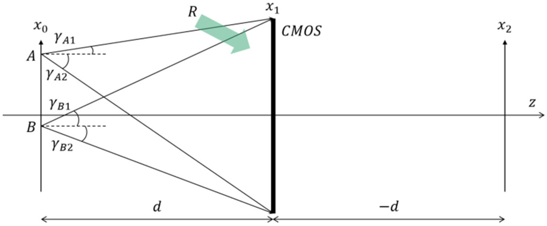
However, although the diffraction-limited optical system is linear, it is not space-invariant [3,25]. Without loss of generality, only the one-dimensional imaging process is considered. Taking holography as an example, Figure 1 shows the recording and reconstruction process of Fresnel holography, where R is the reference wave. For simplicity, the back-propagation is represented to the right. The planes , , and represent the object plane, the CMOS chip (or hologram plane), and the observation plane, respectively.
From the angular spectrum point of view, diffraction in free space occurs from the object plane to the CMOS chip, but due to the finite aperture, the CMOS will only selectively receive the frequency components of each object point. In Figure 1, the frequency components of A and B recorded by the CMOS are different, and the response on the observation plane markedly differs. In other words, the wavelet emitted by different positions of the object plane received by the CMOS is different. Therefore, diffraction-limited optical systems are space-variant systems.
Considering the object field , diffraction from the object plane to the hologram plane is expressed using the Fresnel diffraction formula as follows:
where is the recording distance, is the reconstruction distance, and . If the object field has a rectangular boundary and the side length is , then , where represents the rectangular window function. Let the reference wave be
where , , and . The hologram can then be obtained from the interference between the object wave and the reference wave:
By phase shifting or applying the off-axis technique, the object wave recorded by the hologram can be extracted. Through back-propagation, the reconstructed wave front can be written as
where is the rectangular window function determined by the size of the CMOS chip, which can be regarded as the aperture stop of the Fresnel holographic imaging system. Ignoring the constant term in Equation (7), we can derive the reconstructed wave front as
where is the physical size of the CMOS chip; and represent the Fourier transform and inverse Fourier transform, respectively; is the frequency-domain coordinates after the Fourier transform; and is the spatial-domain coordinates after the inverse Fourier transform.
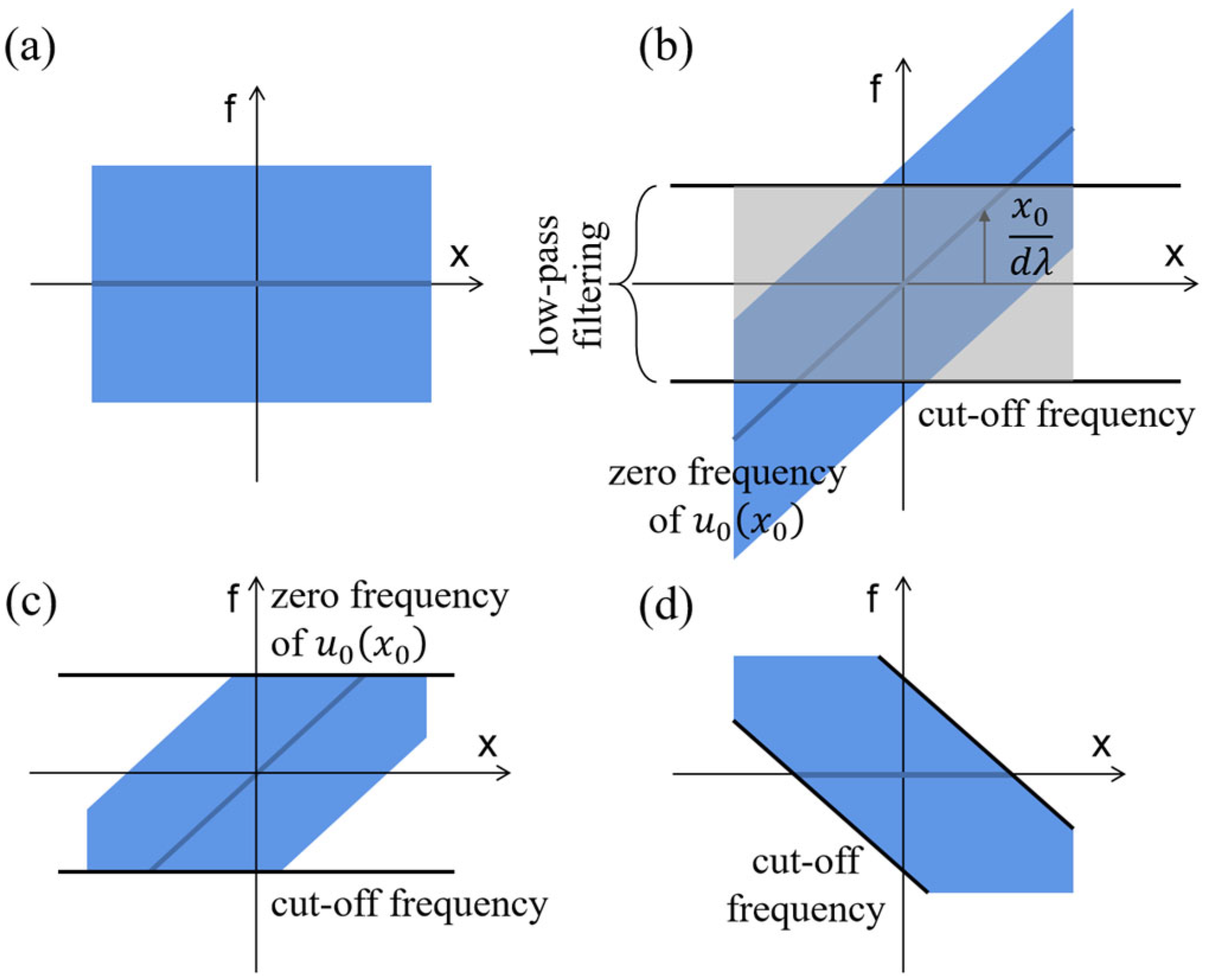
The system represented by Equation (5) is shown in Figure 2 as a block diagram. According to communication theory, the input signal, namely, the object field , is the modulation signal, and its spectrum distribution in phase space is shown in Figure 3a [26,27]. is the carrier signal, which is also called the LFM signal or chirp signal. is the modulated signal. The Fresnel holographic imaging system consists of the following three parts:
- (1)
- Modulation of input signal by carrier signal . If , the frequency shift introduced by the carrier signal when applying the frequency shift theorem of the Fourier transform isEquation (6) shows that the frequency shift is dependent on the spatial coordinates, which indicates that this process is space-variant. The distribution of the modulated signal in phase space is shown in Figure 3b.
- (2)
- Ideal low-pass filtering of modulated signal . represents a rectangular ideal low-pass filter, as shown in Figure 4, whose passband is determined by the angular aperture of the CMOS target plane, namely, . As shown in Figure 3b,c, after the frequency shift of the modulation signal, the original low-frequency information becomes high-frequency. In this case, low-pass filtering will block the original low-frequency information of the modulation signal . The farther away it is from the optical axis, the more low-frequency information of the modulation signal that will be lost. Therefore, for the input signal of the system–object field , the aperture is not reflected as an ideal low-pass filter due to the frequency shift effect of Equation (6) but as a frequency-selective filter, with the constant passband width and center frequency changing with the position in the object plane. Such a filter presents different frequency responses with different spatial locations of the modulation signal ; that is, the filtering process is space-variant for the modulation signal .
- (3)
- Modulation of ideal low-pass-filtered signal by carrier signal . When the reconstruction distance is equal to the recording distance, the two carrier signals before and after filtering are conjugate and cancel each other, and the Fresnel holography reconstruction automatically completes the demodulation process. Therefore, the problem of quadratic phase aberration is not encountered in Fresnel holography. The distribution of the reconstructed wave field in phase space is shown in Figure 3d.
The above analyses reveal that LFM and ideal low-pass filtering are critical to the space-variance effect. Without LFM, the ideal low-pass filtering is strict with respect to the object field, and the system will be space-invariant. Moreover, without ideal low-pass filtering, the two carriers will cancel out, and the reconstructed wave front will not differ from the object wave field.
Both LFM and ideal low-pass filtering are important for space-variance effects, but different optical systems require different considerations. For example, the space-variance effect can be effectively suppressed by using larger optical elements to increase the passband width of the low-pass filter. Usually, this requirement is easy to fulfill, such as by using a larger lens. However, in some cases, such as the demand for a more compact design or when some optical elements are very small, one can only rely on the control of LFM to suppress the space-variance effect. For example, in digital holography, the size of CMOS chips is usually very small, about a few millimeters.
2.2. Three Stages of the Space-Variance Effect
The solution to Equation (5) is derived to further analyze the space-variance effect. From the perspective of signal processing, the chirp rate of the LFM signal is , its bandwidth is , and its space–bandwidth product is . The object wave field is assumed to be a slowly varying function compared with the LFM signal ; therefore, it can be ignored. This approximation is reasonable for phase-only samples with slow phase changes, such as cells. The modulated signal can be reduced to , and its Fourier transform is
Assuming that , , we have
The integral term of Equation (8) is the Fresnel integral, where
The spectrum of the signal is
where
As shown in Figure 4, the red line is the magnitude spectrum of with a rectangular envelope, and its main energy is relatively evenly distributed between and , rather than concentrated near the zero frequency such as in the classical distribution of the magnitude spectrum [28]. This phenomenon is called central frequency spreading [29,30]. Equation (10) offers a good approximation of the spectrum of the modulated signal . Notably, the spectrum is only meaningful in the system represented in Equation (5) or Figure 2 and is independent of the object wave recorded by the hologram.
The low-pass-filtering process can be divided into three states.
- (1)
- Approximate space-invariance state. In this state, the filter passband width is much larger than the bandwidth of the LFM signal; that is, the width of the aperture is much larger than the width of the object field . The blue box in Figure 4 represents the passband of the low-pass filter in this case. Tichenor and Goodman [5] pointed out that when , the space-variance effect is negligible. The classical Fourier optical analysis of optical imaging systems rests on the assumption of approximate space invariance; in other words, only the case is considered.
- (2)
- High-frequency distortion state. The passband width of the filter in this state satisfies . The purple box in Figure 4 represents the passband of the low-pass filter in this case. The energy blocked by the filter is mainly from the high-frequency information of the object field far from the optical axis. The farther away the object wave field is from the optical axis, the higher the frequency modulated by the LFM signal is. Therefore, more information is lost in these areas after low-pass filtering, and the image quality is worse, which is mainly reflected in the distortion of the abrupt phase in the margin of the image wave field.
- (3)
- Boundary-diffraction state. The green box in Figure 4 represents the passband of the low-pass filter when . In this case, the high-frequency information and a mass of low-frequency information in the margin of the object wave field are filtered out. Because the main energy of the optical field is concentrated in the low-frequency information, high energy loss occurs in areas where low-frequency information is filtered out, which leads to a decrease in the signal-to-noise ratio, resulting in phase distortion.
When the space–bandwidth product of the LFM signal is sufficiently large, the spectrum can be approximated as
Equation (12) demonstrates that the spectrum of the band-limited LFM signal can still be regarded as a band-limited LFM signal. Curlander and McDonough [31] pointed out that when the spatial bandwidth product of the LFM signal is greater than 100, Equation (12) is sufficient for obtaining the exact spectrum. Therefore, when the filter passband width is less than the bandwidth of the LFM signal, that is, when the aperture width is less than the object wave field width , ignoring the constant phase, the spectrum after ideal low-pass filtering can be approximated as
The signal presented in Equation (13) is considered a new LFM signal. Let ; its chirp rate is . The bandwidth is the physical width of the aperture. The space–bandwidth product is , which is the same form as the Fresnel number.
The inverse Fourier transform of is
From the derivation in Equations (7)–(10), we can obtain
where
where . Substituting Equation (15) into Equation (5), the quadratic phase factor in Equation (15) cancels out. The reconstructed wave front is
which proves that no quadratic phase aberration is present in the Fresnel-holography-reconstructed wave front. The above derivation assumes that the object field changes slowly, so the solution to Equation (17) can also be regarded as the wavefront error, which is caused by the space-variance effect on the low frequency of the image field.
Equation (17) is obtained from the back-propagation of . The corresponding wavefront error obtained from the forward propagation of is
Equation (18) is exactly the same as the Fresnel diffraction pattern of the square aperture. The square aperture here is the CMOS chip. Therefore, is an instance of the boundary-diffraction state. Moreover, Equations (17) and (18) reveal that the boundary diffraction will disturb the entire image wave field, including the paraxial state.
The experimental results of the three stages of the space-variance effect are shown in Figure 5. The sample is a laser-etched “XJTU” quartz plate with a maximum width of about 3 mm. The size of the CMOS chip used in the experiment is 12.8 × 12.8 (resolution 5120 × 5120, pixel size 2.5 × 2.5 ). Therefore, if the object wave field of the measured sample is exactly located in the center of the CMOS chip, the approximate space-invariance state is satisfied, as shown in Figure 5a. In order to compare the measurement results of the same location of the same sample under different conditions, the sample is moved so that the relative position of the CMOS chip and the object wave field changes, which is equivalent to using a sample with a larger size. If part of the main energy of the object wave field irradiates outside the CMOS chip, the boundary-diffraction state or is satisfied, as shown in Figure 5c. The condition between the cases shown in Figure 5a,c corresponds to the high-frequency distortion state, as shown in Figure 5b.
From the perspective of signal processing, this boundary-diffraction disturbance can be considered a ringing artifact, namely, Gibb’s phenomenon [6]. Cuche et al. [32] utilized the apodization method to suppress the boundary-diffraction disturbance in digital holographic imaging and achieved good results in the application of holographic measurements [33]. In general, in addition to consuming more time and computational resources and having a reduced FOV, the apodization method can satisfactorily suppress the boundary-diffraction perturbation of the intensity map. However, the apodization method does not fundamentally change the space-variance effect of the optical imaging system, so it cannot suppress the high-frequency information distortion in the marginal area of the reconstructed image. In addition, because the apodization method reduces the intensity of the hologram marginal area, the signal-to-noise ratio of the reconstructed image in the corresponding area decreases, which leads to more severe distortion of the phase map.
2.3. Eliminating the Space-Variance Effect by Recording Holograms at the Back Focal Plane of the Imaging Lens
Due to the size of a CMOS chip, the numerical aperture of a Fresnel holographic imaging system is usually much smaller than that of a lens imaging system. Moreover, increasing the numerical aperture by increasing the CMOS chip size is expensive and inefficient. Image holography [22,23] is a hologram-recording method that combines holography with a lens imaging system. We deductively predicted that hologram recording at the back focal plane of the imaging lens would not produce a space-variance effect, and this prediction is proved by simulations and experiments. As shown in Figure 6, if the constant term is ignored, the expression of single-lens imaging is
where is the pupil function, and
where is the focal length of the lens.
In the image holography schematic shown in Figure 7, the image holography consists of single-lens imaging and Fresnel holography when the diffraction between each plane is located in the Fresnel diffraction region. The image formed by the lens can be regarded as the virtual object in Fresnel holography. The recording distance is , and the reconstruction distance is , with their signs being opposite to those in ordinary Fresnel holography. In this case, the formula for Fresnel holographic imaging is as follows:
Substituting Equation (19) into Equation (21) yields a cumbersome expression.
As shown in Figure 8, the optical imaging system presented in Equation (22) can be represented by a block diagram, and the former is analyzed in the phase space, as shown in Figure 9. The modulation of the LFM signal in phase space is manifested as the shearing of the original signal, and the low-pass filtering is manifested as the cutting of the spectrum along the frequency axis. Because shearing occurs before cutting, different states retain different frequency components after cutting, as shown in Figure 9b, which will lead to the space-variance effect. In Figure 7, the virtual object field of holography is the image of the previous lens, which results in the spectrum undergoing reverse shearing and makes it possible to “correct” the spectrum before passing through the next low-pass filter, the CMOS, as shown in Figure 9d. In this case, the frequency response of the CMOS low-pass filter to each spatial position is the same, and no new space-variance effect will be produced.
When
is satisfied, where , that is,
the distance between the lens and the CMOS target plane is
According to Equation (20), we have
and the following formula:
That is, when the distance between the lens and the CMOS chip is the focal length of the lens, the holographic imaging process will not produce a new space-variance effect. In addition, it is necessary to exclude the influence of the lens as much as possible since our focus is on the space-variance effect in digital holography. A large aperture lens can be used to ensure this point. For example, in our experiment, a lens with a diameter of 50.8 mm was used as the image lens, thus satisfying the approximate space-invariance state. When the space-variance effect of the imaging lens can be ignored, the whole holographic imaging system remains space-invariant. From the perspective of Fourier optics, the back focal plane of the imaging lens is the Fourier plane of the object field; thus, the aperture stop located in the back focal plane is equivalent to the ideal low-pass filtering of the object field, so the imaging process is space-invariant. In addition, for different object distances of the same imaging lens, its Fourier plane remains the same, so the recording position of focal plane holography also remains the same.
3. Results
The prediction was verified by simulations and experiments involving microlens array topography measurements. As shown in Figure 10, an ordinary Mach–Zehnder interferometer was used for the experiment. A laser beam with a wavelength of 523.5 nm was used in our experiment; the focal length of the imaging lens was 200 mm, and the sample was placed 400 mm in front of the imaging lens to maintain a vertical-axis magnification of 1×. The tested object was an lbtek MLAS10-F15-P300-AB microlens array with a period of 300 μm and window size of 9 mm × 9 mm. A CMOS camera with a resolution of 5120 × 5120 and pixel size of 2.5 μm was used for recording. To better compare the image quality of the three hologram-recording methods, the holograms were cropped to a resolution of 3800 × 3800 with a physical size of 9.5 mm.
For comparison, the following three sets of simulations and experiments were performed: Fresnel holography, image holography with the recording of holograms at the back focal plane (IHWF), and image holography without recording holograms at the back focal plane of the imaging lens (IHWOF). To maintain the same numerical aperture as that in IHWF, the CMOS was placed 200 mm behind the sample in Fresnel holography and 200 mm behind the image plane of the imaging lens in IHWOF. Calculations show that the recording distance satisfies the Fresnel approximation condition and the spectrum separation condition of off-axis holography.
The simulation processes of Fresnel holography and image holography are based on the block diagrams shown in Figure 2 and Figure 8, and the simulation results under the above conditions are shown in Figure 11 and Figure 12, respectively.
Recording the hologram directly at the back focal plane of the imaging lens in the IHWF experiment is difficult because the energy of the zero-frequency component is too concentrated, and the overexposure of the low-frequency information is severe. Therefore, the CMOS target plane can slightly deviate from the focal plane to record the hologram and still maintain the approximate space invariance.
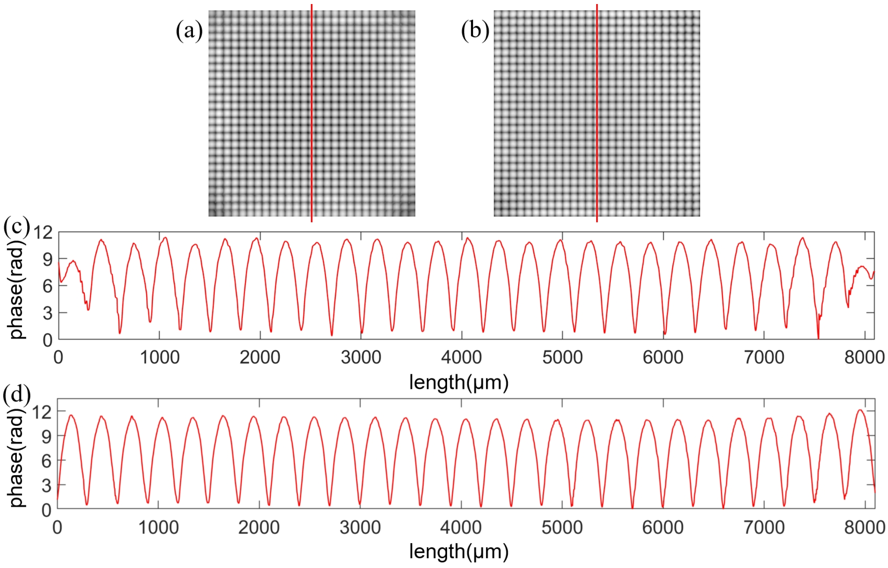
The experimental results are shown in Figure 13 and Figure 14. In Figure 14c, because of the space-variance effect, the high-frequency information at the edge of the microlens array is lost, while the phase in Figure 14d is in order. In addition, there is a phenomenon of a “phase increase” at the edge in Figure 14, which may result from phase aberration. The experimental results in [34,35,36,37,38,39,40] indicate that in digital holographic phase measurement, it is difficult to perfectly control or eliminate the phase aberration in the whole field of view. However, the “phase increase” in Figure 14 does not affect any of the analyses and conclusions of this article.
The simulation and experimental results reveal that the imaging quality of IHWF is significantly higher than that of Fresnel holography and IHWOF, and the imaging quality of IHWOF is worse than that of Fresnel holography. The latter can easily be explained by Figure 8 and Figure 9. For example, the bandwidth of the LFM signal in IHWOF is twice that of the LFM signal in Fresnel holography, so only the area in the center, which occupies approximately 1/4 of the total area in Figure 11k and Figure 13k, has relatively high imaging quality. These results indicate that IHWF has the potential to suppress or even eliminate the space-variance effect and further indicate the correctness of the proposed theory.
4. Discussion
In this article, Fresnel holography and holography with a lens are studied. It is precisely because the object of study is very simple that it is possible to obtain theoretical solutions. However, modern optical systems are often complex and contain a large number of optical elements. Furthermore, different optical elements modulate the beam differently, and the superposition effects are difficult to strictly derive.
It is meaningful to analyze the space-variance effect of complex optical systems to improve the imaging capability of these systems. Unfortunately, these cases are beyond the scope of this article. More research is needed on how the spatial effect will affect the system and what kind of experimental phenomena occur in a system with a large number of optical elements, such as grating and spatial light modulators.
One of the significant contributions of this manuscript is that it provides a good framework: that is, through Fourier analysis and phase space analysis for each step of the diffraction process, the space-variance effect of the whole system is finally obtained. This lays a foundation for the future study of the space-variance effects of complex systems.
5. Conclusions
In this study, the digital holography imaging system is regarded as a space-variant system. In digital Fresnel holography, the space-variance effect severely affects the measurement results due to the small size of the CMOS chip. Therefore, it is inappropriate to treat it as a space-invariant system. The discussion of space-variance effects in Section 2 and Section 3 of this paper is based on Fresnel holography, but it is also applicable to ordinary optical imaging systems. The presented analysis reveals that the space-variance effect is caused by LFM and ideal low-pass filtering. If one of these two conditions is destroyed, the space-variance effect can be eliminated. Furthermore, three states of the space-variance effect are pointed out: approximate space-invariance state, high-frequency distortion state, and boundary-diffraction state. In this study, the two physical phenomena of high-frequency distortion and boundary diffraction are added to the classical Fourier optical analysis of an optical imaging system, which only considers the approximate space-invariance state, making it more consistent with the fact.
Based on the theory proposed in this study, we have proved through theoretical analysis, simulation, and experiments that the space-variance effect can be controlled by adjusting the distance between the optical elements in the imaging system, especially when recording the hologram in the back focal plane of the imaging lens, in which case the holographic imaging process will not produce a new space-variance effect. In other words, when the space-variance effect of the imaging lens can be ignored, there will be no space-variance effect in the imaging system. Thus, this article provides a comprehensive understanding of digital holographic imaging systems with the space-variance effect.
Author Contributions
Conceptualization, X.Y. and R.Z.; methodology, X.Y. and R.Z.; validation, X.Y. and Y.D.; formal analysis, X.Y. and H.C.; investigation, X.Y. and C.F.; resources, X.Y. and Y.D.; data curation, X.Y. and R.Z.; writing—original draft preparation, X.Y.; writing—review and editing, X.Y. and Z.Z; visualization, X.Y. and H.C.; supervision, X.Y. and Z.Z.; project administration, X.Y.; funding acquisition, Z.Z. and G.Z. All authors have read and agreed to the published version of the manuscript.
Funding
This research was funded by the National Natural Science Foundation of China, grant number 52175516, and Youth Innovation Promotion Association, grant number 2022410.
Institutional Review Board Statement
Not applicable.
Informed Consent Statement
Not applicable.
Data Availability Statement
Data can be obtained from the corresponding author upon request.
Conflicts of Interest
The authors declare no conflict of interest.
References
- Goodman, J.W. Introduction to Fourier Optics, 4th ed.; W.H. Freeman: New York, NY, USA, 2017. [Google Scholar]
- Yan, H.; Liu, C.Y.; Jun, L.; Ping, C.; Qian, K.M.; Asundi, A. Investigation of the systematic axial measurement error caused by the space variance effect in digital holography. Opt. Lasers Eng. 2019, 112, 16–25. [Google Scholar] [CrossRef]
- Lohmann, A.W.; Paris, D.P. Space-Variant Image Formation. J. Opt. Soc. Am. 1965, 55, 1007–1013. [Google Scholar] [CrossRef]
- Brainis, E.; Muldoon, C.; Brandt, L.; Kuhn, A. Coherent imaging of extended objects. Opt. Commun. 2009, 282, 465–472. [Google Scholar] [CrossRef]
- Tichenor, D.A.; Goodman, J.W. Coherent Transfer-Function. J. Opt. Soc. Am. 1972, 62, 293–295. [Google Scholar] [CrossRef]
- Pan, A.; Zuo, C.; Xie, Y.G.; Lei, M.; Yao, B.L. Vignetting effect in Fourier ptychographic microscopy. Opt. Lasers Eng. 2019, 120, 40–48. [Google Scholar] [CrossRef]
- Girshovitz, P.; Shaked, N.T. Fast phase processing in off-axis holography using multiplexing with complex encoding and live-cell fluctuation map calculation in real-time. Opt. Express 2015, 23, 8773–8787. [Google Scholar] [CrossRef]
- Merola, F.; Memmolo, P.; Miccio, L.; Savoia, R.; Mugnano, M.; Fontana, A.; D’Ippolito, G.; Sardo, A.; Iolascon, A.; Gambale, A.; et al. Tomographic flow cytometry by digital holography. Light-Sci. Appl. 2017, 6, 7. [Google Scholar] [CrossRef]
- Tahara, T.; Quan, X.Y.; Otani, R.; Takaki, Y.; Matoba, O. Digital holography and its multidimensional imaging applications: A review. Microscopy 2018, 67, 55–67. [Google Scholar] [CrossRef]
- Katz, J.; Sheng, J. Applications of Holography in Fluid Mechanics and Particle Dynamics. Annu. Rev. Fluid Mech. 2010, 42, 531–555. [Google Scholar] [CrossRef]
- Miccio, L.; Memmolo, P.; Merola, F.; Fusco, S.; Embrione, V.; Paciello, A.; Ventre, M.; Netti, P.A.; Ferraro, P. Particle tracking by full-field complex wavefront subtraction in digital holography microscopy. Lab Chip 2014, 14, 1129–1134. [Google Scholar] [CrossRef]
- Chen, Y.; Guildenbecher, D.R.; Hoffmeister, K.N.G.; Cooper, M.A.; Stauffacher, H.L.; Oliver, M.S.; Washburn, E.B. Study of aluminum particle combustion in solid propellant plumes using digital in-line holography and imaging pyrometry. Combust. Flame 2017, 182, 225–237. [Google Scholar] [CrossRef]
- Khmaladze, A.; Restrepo-Martinez, A.; Kim, M.; Castaneda, R.; Blandon, A. Simultaneous dual-wavelength reflection digital holography applied to the study of the porous coal samples. Appl. Opt. 2008, 47, 3203–3210. [Google Scholar] [CrossRef] [PubMed]
- Kuhn, J.; Charriere, F.; Colomb, T.; Cuche, E.; Montfort, F.; Emery, Y.; Marquet, P.; Depeursinge, C. Axial sub-nanometer accuracy in digital holographic microscopy. Meas. Sci. Technol. 2008, 19, 8. [Google Scholar] [CrossRef]
- Agour, M.; Falldorf, C.; Bergmann, R.B. Spatial multiplexing and autofocus in holographic contouring for inspection of micro-parts. Opt. Express 2018, 26, 28576–28588. [Google Scholar] [CrossRef] [PubMed]
- Kostencka, J.; Kozacki, T.; Kus, A.; Kemper, B.; Kujawinska, M. Holographic tomography with scanning of illumination: Space-domain reconstruction for spatially invariant accuracy. Biomed. Opt. Express 2016, 7, 4086–4101. [Google Scholar] [CrossRef] [PubMed]
- Balasubramani, V.; Kus, A.; Tu, H.Y.; Cheng, C.J.; Baczewska, M.; Krauze, W.; Kujawinska, M. Holographic tomography: Techniques and biomedical applications Invited. Appl. Opt. 2021, 60, B65–B80. [Google Scholar] [CrossRef] [PubMed]
- Cuche, E.; Bevilacqua, F.; Depeursinge, C. Digital holography for quantitative phase-contrast imaging. Opt. Lett. 1999, 24, 291–293. [Google Scholar] [CrossRef]
- Mann, C.J.; Yu, L.F.; Lo, C.M.; Kim, M.K. High-resolution quantitative phase-contrast microscopy by digital holography. Opt. Express 2005, 13, 8693–8698. [Google Scholar] [CrossRef]
- Mohammed, S.K.; Bouamama, L.; Bahloul, D.; Picart, P. Quality assessment of refocus criteria for particle imaging in digital off-axis holography. Appl. Opt. 2017, 56, F158–F166. [Google Scholar] [CrossRef]
- Yamagiwa, M.; Minamikawa, T.; Trovato, C.; Ogawa, T.; Ibrahim, D.G.A.; Kawahito, Y.; Oe, R.; Shibuya, K.; Mizuno, T.; Abraham, E.; et al. Multicascade-linked synthetic wavelength digital holography using an optical- comb-referenced frequency synthesizer. Opt. Express 2018, 26, 26292–26306. [Google Scholar] [CrossRef]
- Cuche, E.; Marquet, P.; Depeursinge, C. Simultaneous amplitude-contrast and quantitative phase-contrast microscopy by numerical reconstruction of Fresnel off-axis holograms. Appl. Opt. 1999, 38, 6994–7001. [Google Scholar] [CrossRef] [PubMed]
- Colomb, T.; Cuche, E.; Charriere, F.; Kuhn, J.; Aspert, N.; Montfort, F.; Marquet, P.; Depeursinge, C. Automatic procedure for aberration compensation in digital holographic microscopy and applications to specimen shape compensation. Appl. Opt. 2006, 45, 851–863. [Google Scholar] [CrossRef]
- Hecht, E. Optics, Global, 5th ed.; Pearson: Boston, MA, USA, 2017. [Google Scholar]
- Stein, A.; Barbastathis, G. Axial imaging necessitates loss of lateral shift invariance. Appl. Opt. 2002, 41, 6055–6061. [Google Scholar] [CrossRef] [PubMed]
- Bastiaans, M.J. Application of the Wigner Distribution Function in Optics. In The Wigner Distribution—Theory and Applications in Signal Processing; Mecklenbräuker, W., Hlawatsch, F., Eds.; Elsevier: Amsterdam, The Netherlands, 1997; pp. 375–426. Available online: https://research.tue.nl/en/publications/application-of-the-wigner-distribution-function-in-optics (accessed on 29 November 2023).
- Oh, S.B.; Barbastathis, G. Axial imaging necessitates loss of lateral shift invariance: Proof with the Wigner analysis. Appl. Opt. 2009, 48, 5881–5888. [Google Scholar] [CrossRef] [PubMed]
- Gonzalez, R.C.; Woods, R.E. Digital Image Processing; Pearson: New York, NY, USA, 2018; p. xvi. 1168p. [Google Scholar]
- Colomb, T.; Montfort, F.; Kuhn, J.; Aspert, N.; Cuche, E.; Marian, A.; Charriere, F.; Bourquin, S.; Marquet, P.; Depeursinge, C. Numerical parametric lens for shifting, magnification, and complete aberration compensation in digital holographic microscopy. J. Opt. Soc. Am. A Opt. Image Sci. Vis. 2006, 23, 3177–3190. [Google Scholar] [CrossRef] [PubMed]
- Zuo, C.; Chen, Q.; Qu, W.J.; Asundi, A. Phase aberration compensation in digital holographic microscopy based on principal component analysis. Opt. Lett. 2013, 38, 1724–1726. [Google Scholar] [CrossRef] [PubMed]
- Curlander, J.C.; McDonough, R.N. Synthetic Aperture Radar: Systems and Signal Processing; John Wiley & Sons, Inc: New York, NY, USA, 1991; p. xvii. 647p. [Google Scholar]
- Cuche, E.; Marquet, P.; Depeursinge, C. Aperture apodization using cubic spline interpolation: Application in digital holographic microscopy. Opt. Commun. 2000, 182, 59–69. [Google Scholar] [CrossRef]
- Kuhn, J.; Niraula, B.; Liewer, K.; Wallace, J.K.; Serabyn, E.; Graff, E.; Lindensmith, C.; Nadeau, J.L. A Mach-Zender digital holographic microscope with sub-micrometer resolution for imaging and tracking of marine micro-organisms. Rev. Sci. Instrum. 2014, 85, 6. [Google Scholar] [CrossRef]
- Wen, Y.F.; Qu, W.J.; Cheng, H.B.; Yan, H.; Asundi, A. Further investigation on the phase stitching and system errors in digital holography. Appl. Opt. 2015, 54, 266–276. [Google Scholar] [CrossRef]
- Zhang, X.L.; Zhang, X.C.; Xu, M.; Zhang, H.; Jiang, X.Q. Phase unwrapping in digital holography based on non-subsampled contourlet transform. Opt. Commun. 2018, 407, 367–374. [Google Scholar] [CrossRef]
- Ren, Z.B.; Zhao, J.L.; Lam, E.Y. Automatic compensation of phase aberrations in digital holographic microscopy based on sparse optimization. APL Photonics 2019, 4, 110808. [Google Scholar] [CrossRef]
- Liu, B.C.; Feng, D.Q.; Feng, F.; Tian, A.L.; Liu, W.G. Maximum a posteriori-based digital holographic microscopy for high-resolution phase reconstruction of a micro-lens array. Opt. Commun. 2020, 477, 126364. [Google Scholar] [CrossRef]
- Zheng, C.; Jin, D.; He, Y.P.; Lin, H.T.; Hu, J.J.; Yaqoob, Z.; So, P.T.C.; Zhou, R.J. High spatial and temporal resolution synthetic aperture phase microscopy. Adv. Photonics 2020, 2, 065002. [Google Scholar] [CrossRef] [PubMed]
- Zhong, Z.; Zhao, H.J.; Shan, M.G.; Liu, B.; Lu, W.L.; Zhang, Y.B. Off-axis digital holographic microscopy with divided aperture. Opt. Lasers Eng. 2020, 127, 105954. [Google Scholar] [CrossRef]
- Fan, X.; Healy, J.J.; O’Dwyer, K.; Winnik, J.; Hennelly, B.M. Adaptation of the Standard Off-Axis Digital Holographic Microscope to Achieve Variable Magnification. Photonics 2021, 8, 264. [Google Scholar] [CrossRef]
Figure 1.
The recording and reconstruction process of Fresnel holography. A and B are any two points on the plane .
Figure 1.
The recording and reconstruction process of Fresnel holography. A and B are any two points on the plane .

Figure 2.
The block diagram of Fresnel holographic imaging system.

Figure 3.
Distribution of spectrum in phase space for each step in Figure 2. The f-axis is the frequency, and the x-axis is the spatial coordinate. (a) The spectrum distribution of the object field in phase space. The thick blue line is the zero-frequency component of the object field . (b) The spectrum distribution of the modulated signal in phase space, which can be obtained by shearing (a) by . The thick black line is the cut-off frequency. (c) Distribution of spectrum in phase space after ideal low-pass filtering. (d) The spectrum distribution of the reconstructed wave field in phase space, which can be obtained by shearing (c) by .

Figure 4.
Schematic of the amplitude spectrum of spectrum .
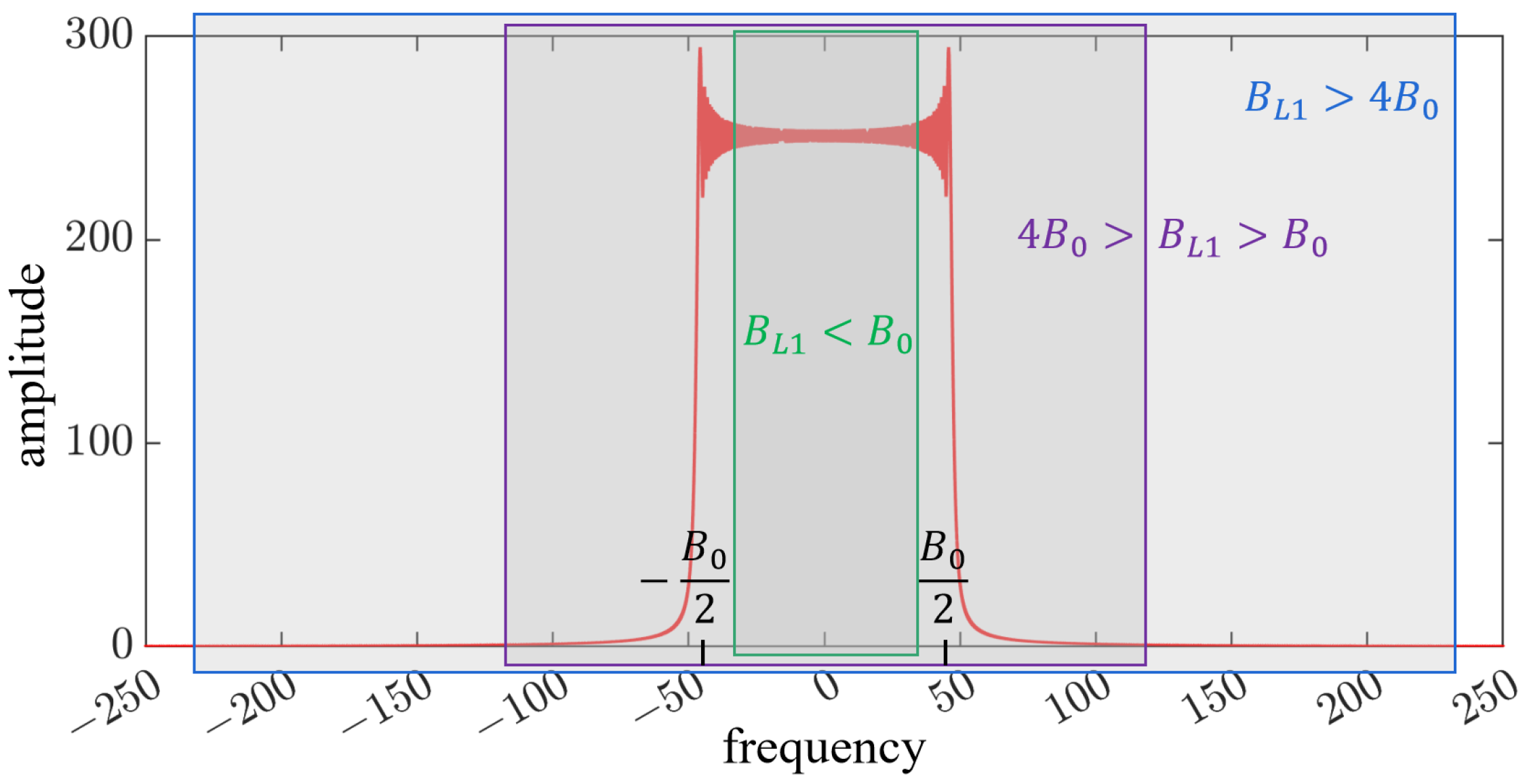
Figure 5.
Fresnel holographic measurements in the three stages of space-variance effect. (a–c) are Fresnel holograms recorded under three conditions: the diffraction wave field of the measured object falls on the center of the CMOS target plane; it falls to the right, but the main part is still on the CMOS target plane; and part of the direct light does not fall on the CMOS target plane. (d–f) represent the reconstructed intensity map of the three aforementioned holograms and zero padding to 7500 × 7500 pixels during reconstruction. (g–i) are enlarged views of the red-boxed areas in (d–f). Distinct boundary-diffraction fringes or ringing artifacts are evident in (i). (j–l) are the phase diagrams corresponding to the red-boxed areas in (g–i). (m–o) are the contour lines at the red lines in figures (j–l). (n) shows the phase distortion at the step, which is caused by the loss of high-frequency information here due to the space-variance effect. (o) shows the perturbation of the low-frequency information by boundary diffraction, and the overall trend of the contour being severely affected.

Figure 6.
Schematic of single-lens imaging. and are object and image distances, respectively; and are focal points; , , and are the coordinates of the object, lens, and image planes, respectively.
Figure 6.
Schematic of single-lens imaging. and are object and image distances, respectively; and are focal points; , , and are the coordinates of the object, lens, and image planes, respectively.

Figure 7.
Schematic of image holography. and are the object and image distances of the lens, respectively. The CMOS is located between the lens and the image plane, is the distance between the CMOS and the image plane, and is the distance between the lens and CMOS. and are the front and back focal points of the lens, respectively. , , and are the lens object, lens, and lens image planes, respectively. is also the object plane of the holographic imaging system, which can be regarded as the virtual object. and are the CMOS and reconstructed image planes, respectively. In this case, lies between and , and coincides with .
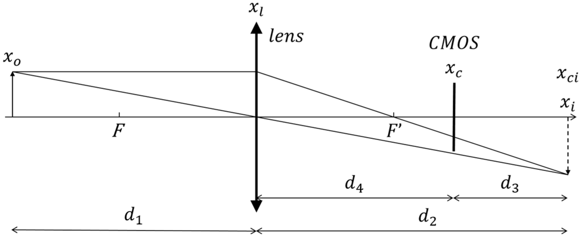
Figure 8.
Block diagram of the image holographic system shown in Figure 7 and Equation (22).
Figure 8.
Block diagram of the image holographic system shown in Figure 7 and Equation (22).
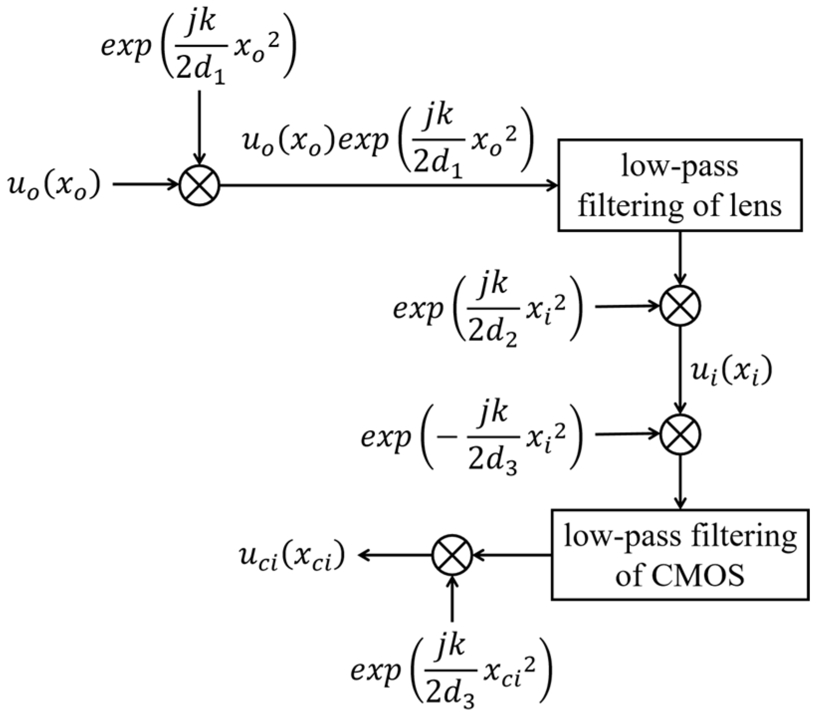
Figure 9.
Distribution of the spectrum in the phase space for each step in Figure 8. The f-axis is the frequency, and the x-axis is the spatial coordinate. The thick blue line represents the zero-frequency component of the object field . (a) The modulation of the object field by the LFM signal is represented by shearing (rather than rotation) in the upper right and lower left or counterclockwise direction, after which the original low-frequency component linearly spreads to the high frequency. (b) The result of low-pass filtering of the modulated signal . (c) Further modulation by the LFM signal . (d) The modulation effect of the LFM signal is represented by the upper left and lower right or clockwise shearing, unlike the former two. In this figure, cancels the previous two steps of modulation, and the spectrum returns to its original position.
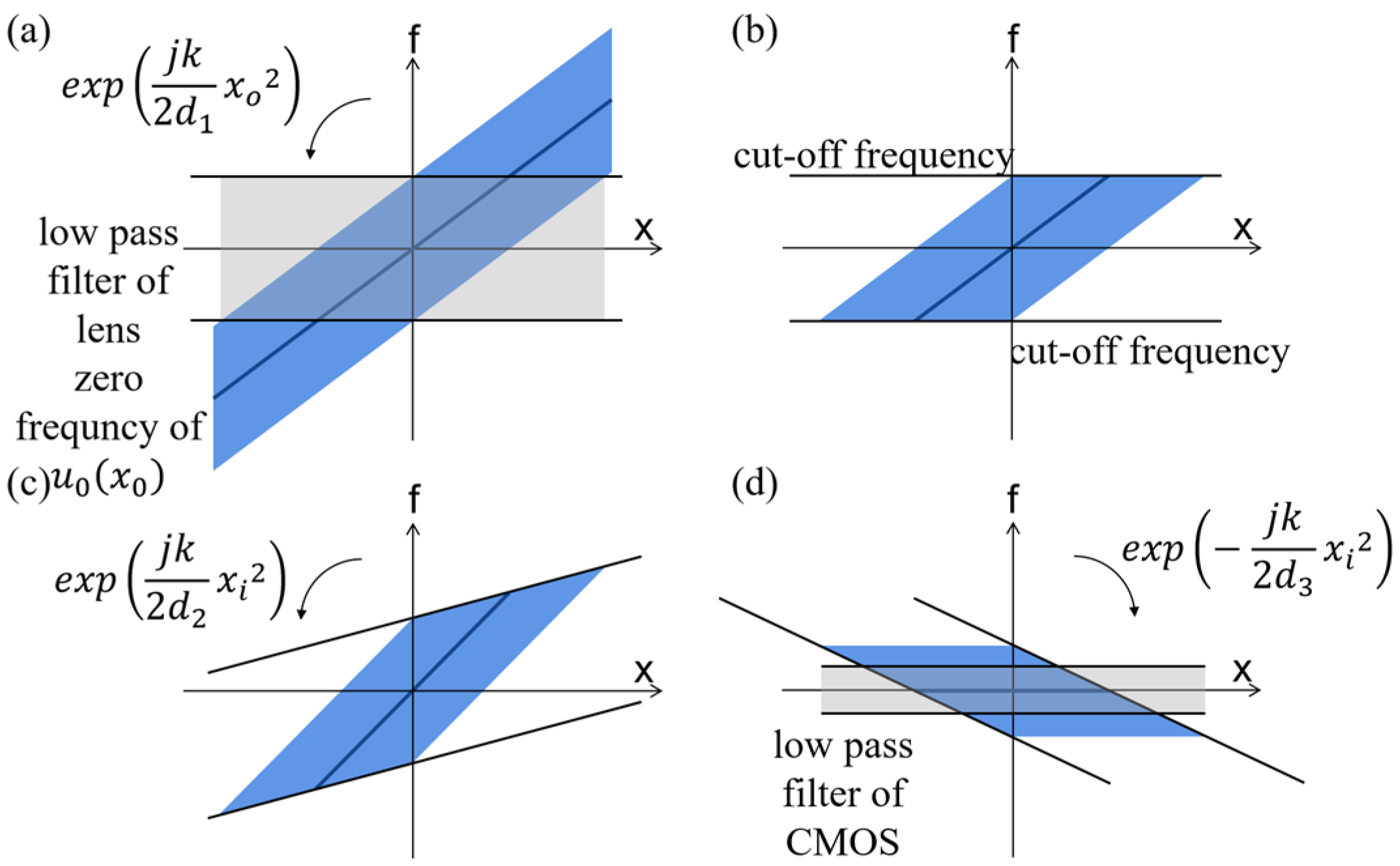
Figure 10.
Schematic of the image holography. BE, beam expander with spatial filter; BS, beam splitter; M, plane mirror; L, imaging lens; d1, object distance; d4, distance between lens and CMOS; f, focal length of the lens L.
Figure 10.
Schematic of the image holography. BE, beam expander with spatial filter; BS, beam splitter; M, plane mirror; L, imaging lens; d1, object distance; d4, distance between lens and CMOS; f, focal length of the lens L.
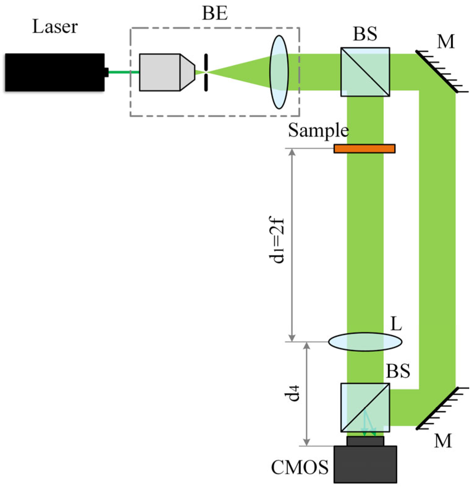
Figure 11.
(a–l) are the simulation results of microlens array measurements obtained using Fresnel holography, IHWF, and IHWOF, respectively. (a,e,i) are the intensity maps. (b,f,j) are the wrapped phase maps; (c) is the enlarged image of the area in the red box in (b); and (g,k) are the wrapped phase maps after compensating for the phase aberration of the area in the red boxes in (f,j), respectively. (d,h,l) are the enlarged images in the red boxes in (c,g,k), respectively.
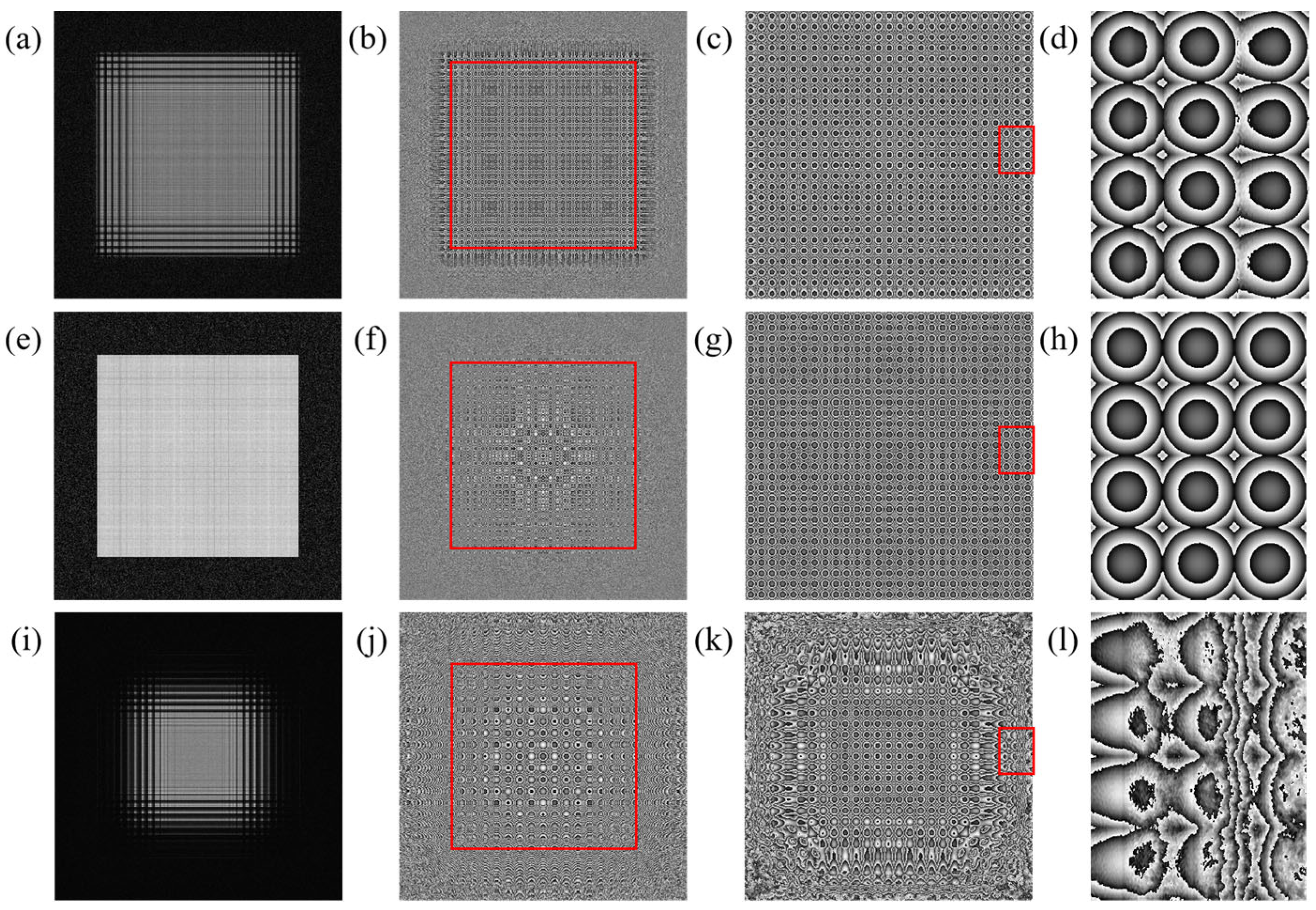
Figure 12.
Simulation results. (a,b) show the unwrapped phase maps of Fresnel holography and IHWF reconstructed wave front, respectively (unwrapped results of the phase maps in Figure 11c,g, respectively). (c,d) represent the profile curves at the red lines in (a,b), respectively.
Figure 12.
Simulation results. (a,b) show the unwrapped phase maps of Fresnel holography and IHWF reconstructed wave front, respectively (unwrapped results of the phase maps in Figure 11c,g, respectively). (c,d) represent the profile curves at the red lines in (a,b), respectively.
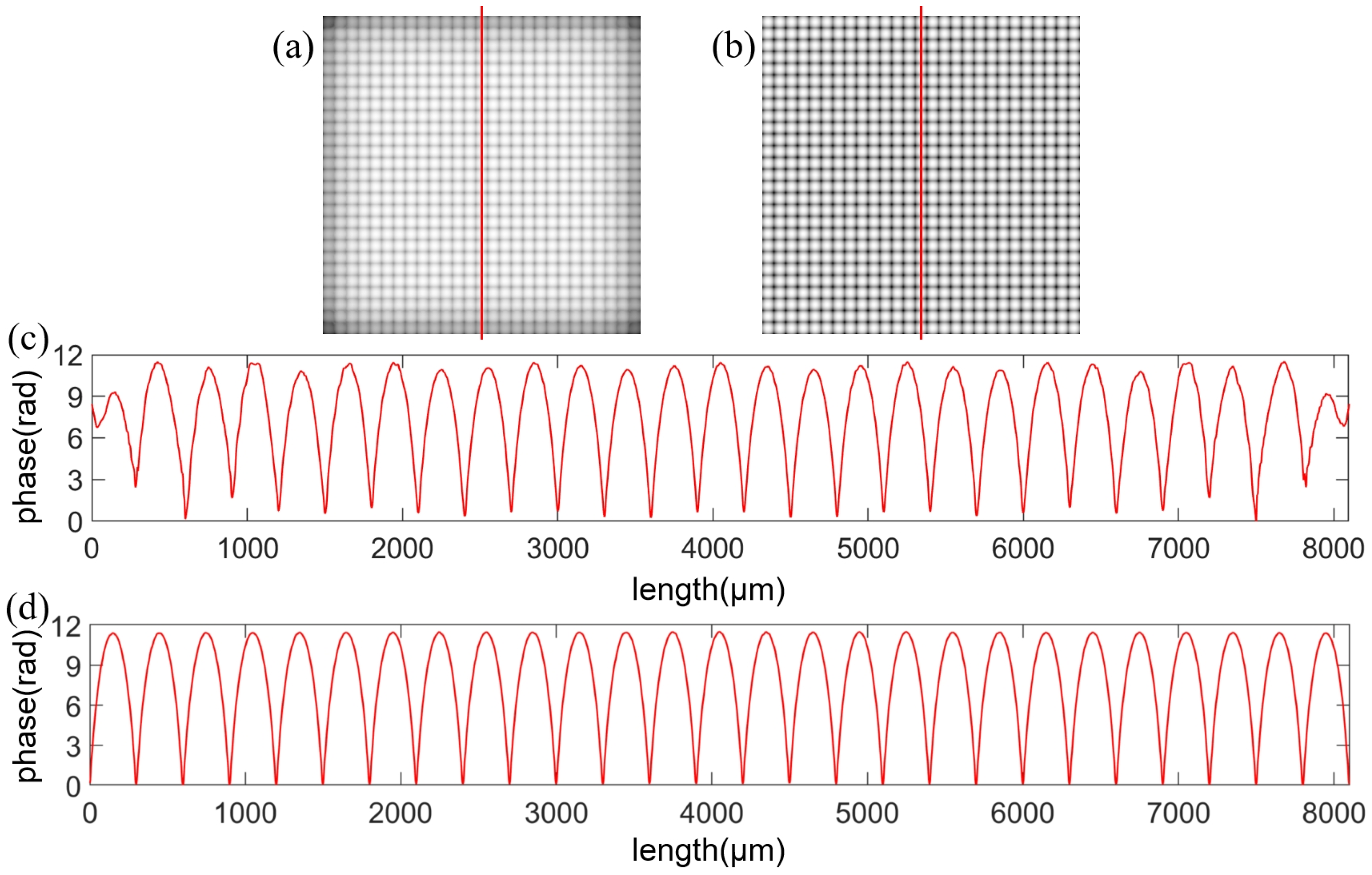
Figure 13.
(a–l) are the experimental results of microlens array measurements for Fresnel holography, IHWF, and IHWOF, respectively. (a,e,i) are the intensity maps. (b,f,j) are the wrapped phase maps; (c) is the enlarged image of the area in the red box in (b); and (g,k) are the wrapped phase maps after compensating for the phase aberration of the areas in the red boxes in (f,j), respectively. (d,h,l) are the enlarged images in the red boxes in (c,g,k), respectively.
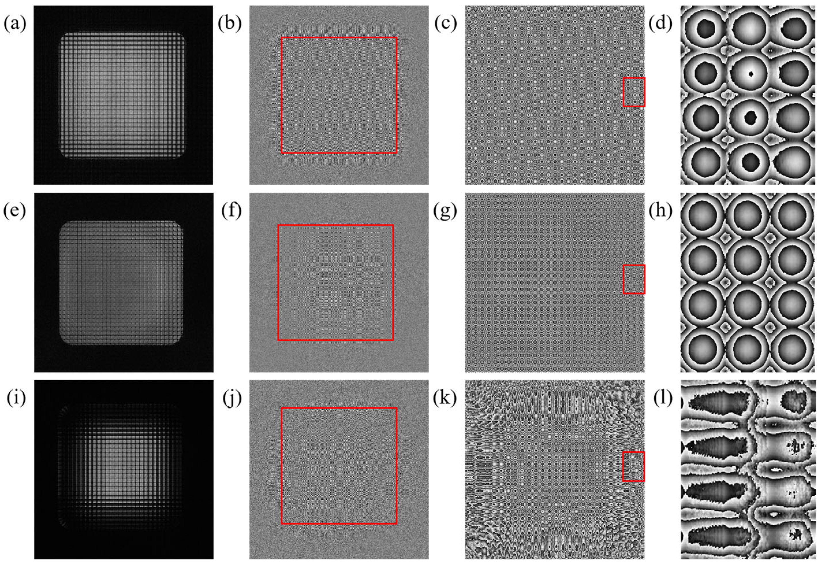
Figure 14.
Experimental results. (a,b) show the unwrapped phase maps of Fresnel-holography- and IHWF-reconstructed wave fronts, respectively (unwrapped results of the phase maps in Figure 13c,g, respectively). (c,d) are the profile curves at the red lines in (a,b), respectively.
Figure 14.
Experimental results. (a,b) show the unwrapped phase maps of Fresnel-holography- and IHWF-reconstructed wave fronts, respectively (unwrapped results of the phase maps in Figure 13c,g, respectively). (c,d) are the profile curves at the red lines in (a,b), respectively.
Disclaimer/Publisher’s Note: The statements, opinions and data contained in all publications are solely those of the individual author(s) and contributor(s) and not of MDPI and/or the editor(s). MDPI and/or the editor(s) disclaim responsibility for any injury to people or property resulting from any ideas, methods, instructions or products referred to in the content. |
© 2023 by the authors. Licensee MDPI, Basel, Switzerland. This article is an open access article distributed under the terms and conditions of the Creative Commons Attribution (CC BY) license (https://creativecommons.org/licenses/by/4.0/).
Share and Cite
MDPI and ACS Style
Yang, X.; Zhao, R.; Chen, H.; Du, Y.; Fan, C.; Zhang, G.; Zhao, Z. Investigation of the Space-Variance Effect of Imaging Systems with Digital Holography. Photonics 2023, 10, 1350. https://doi.org/10.3390/photonics10121350
AMA Style
Yang X, Zhao R, Chen H, Du Y, Fan C, Zhang G, Zhao Z. Investigation of the Space-Variance Effect of Imaging Systems with Digital Holography. Photonics. 2023; 10(12):1350. https://doi.org/10.3390/photonics10121350
Chicago/Turabian StyleYang, Xingyu, Rong Zhao, Huan Chen, Yijun Du, Chen Fan, Gaopeng Zhang, and Zixin Zhao. 2023. "Investigation of the Space-Variance Effect of Imaging Systems with Digital Holography" Photonics 10, no. 12: 1350. https://doi.org/10.3390/photonics10121350
Note that from the first issue of 2016, this journal uses article numbers instead of page numbers. See further details here.