Storage Duration Prediction for Long-Expired Frozen Meat Exceeding State Reserve Time via Swept-Source Optical Coherence Tomography (SS-OCT) under Low-Frequency Electric Field

Abstract

Storage duration detection for frozen meat, especially meat exceeding the state reserve time several times, has always been a big challenge in food safety inspection. Under long freezing times, the physical and chemical properties of meat change complexly. In this paper, the SS-OCT detection method under a low-frequency electric field is firstly (to our knowledge) applied to the predict storage durations of long-expired frozen meat. The average normalized cross-correlation (ANCC) is put forward as a comprehensive parameter to reflect both the electric–kinetic and optical properties of meat’s biological changes. A monotonically increasing inversion rule between ANCC and the storage duration of frozen meat is found after investigating 3840 pork samples, the frozen storage durations of which were from 1 to 13 months. To verify the correctness and accuracy of our method, nine groups of long-expired frozen pork samples were investigated. The maximum relative error for their storage durations is less than 5.71%, which means that our SS-OCT method under a low-frequency electric field is promising in providing a rapid on-site storage duration detection method without any complicated laboratory pretreatments for food safety inspection.

1. Introduction

The main components of meat are water (50%~70%), protein (10%~20%), fat (10%~30%) and carbohydrate (1%~5%) [1], which gradually change during frozen storage and finally influence the freshness and quality of meat. In the world, most countries have standardized the storage time for their state reserve meat. The average storage time, using pork as an example, is about 4 months. Once the storage duration of frozen meat exceeds it, some potential bio-safety issues may arise in terms of the food safety. It has been reported [2] that water holding capacity and protein solubility decrease after chicken breast meat is stored at −20 °C for 3 months, and on the other hand the content of thiobarbituric acid active substances increases obviously. The quality of mutton stored at −18 °C for 21 months has been proven to become worse due to the decrease in the redness and water holding capacity, and the increase in yellowness and lipid oxidation [3]. For pork and beef refrigerated at a temperature of 0 °C~4 °C for two weeks, their total plate counts (TPCs) increase, which is found to have a close correlation with the volatile base nitrogen (VBN) and D-glucose content. In addition, some other changes also occur including increasing protein degradation, fat oxidation and conductivity [4]. As the duration of frozen storage becomes longer, meat’s physical and chemical properties change, which poses a potential threat to food safety. Therefore, it is of great significance to predict the duration of the frozen storage of meat, especially for long-expired meat exceeding the state reserve time several times.

Optical imaging methods have been attempted to estimate the freshness and quality of frozen meat, such as near-infrared spectroscopy, hyper-spectral imaging and ultrasound imaging [5,6,7], via which freezing rate [5], drip loss [6] and protein content [7] have been detected. However, some of them such as hyper-spectral imaging are limited to surface examination [5]. Additionally, the complex operations and professional laboratory conditions result in a tradeoff between resolution and speed. Optical coherence tomography (OCT), as another kind of optical imaging method, can rapidly provide not only 2D cross-sectional but also 3D volumetric images of the inside of biological samples. Based on the light backscattered from different layers within the sample, biological structural information can be recorded at a micron-level resolution and within millimeters of imaging depth. Compared to other imaging technologies, OCT technology has better tomography capabilities. Both real-time detection and high-resolution tomography can be therefore successfully performed [8]. As a result, these methods have drawn attention in frozen meat safety inspection [9,10,11]. For example, intramuscular fat content has been estimated via OCT [9]. Additionally, it has been proven that fat absorbs infrared light in an amount that is nine times higher than muscle does based on polarization-sensitive OCT results [10].

Recently, OCT has been applied for monitoring the electro-kinetic response of biological tissues [12,13]. The biological tissue alterations influenced by electric fields are found to have a close relationship with their physiologies, such as the changes in cell shapes and orientation. As typical ex vivo biological tissues, chicken breast samples under temperature conditions of 0 °C, 4 °C, and 8 °C for 8 days are detected via OCT with external electric field excitation to assess their freshness. Unfortunately, frozen meat kept under −20 °C for different storage durations has seldom been studied.

In this study, we try to apply the electro-kinetic response imaged via OCT to determine the storage durations of frozen meat. To obtain the real-time electro-kinetic response of meat biological properties under a low-frequency electric field, OCT should satisfy some requirements: (1) a rapid measurement speed for the measurement of the real-time electro-kinetic response of frozen meat; (2) a good penetration depth for obtaining more information on the inside of frozen meat along the vertical direction; (3) a high resolution for recording the electro-kinetic response inside meat. As we all know, swept-source OCT (SS-OCT) compared to traditional time-domain OCT (TD-OCT) in Fourier-domain optical coherence tomography has better imaging sensitivity, range and speed, which can meet these requirements well [11]. Therefore, it has been widely used for morphological and functional examinations of biological tissues.

In this paper, SS-OCT under a low-frequency electric field is firstly (to the best of our knowledge) put forward for frozen meat storage duration detection. Frozen pork samples stored for a duration within and exceeding 3 times the state reserve time are investigated. The electro-kinetic response of frozen meat and low-frequency electric fields propagating in it have been observed and imaged. The parameter named average normalized cross-correlation (ANCC) is developed and proven to be sensitive to frozen storage duration. The experimental results present that SS-OCT under a low-frequency electric field can be used for the on-site observation and quantitative evaluation of the storage duration of long-expired frozen meat without any complicated pretreatment or specialized laboratory conditions.

2. Materials and Methods

2.1. Meat Sample

An amount of 1 kg of fresh pork tenderloins from locally produced pig breeds (Guanzhong pig, Shaanxi, China) is purchased once a month and transported to our laboratory at room temperature. The fascia on the surface of pork meat is removed. The muscle parts with trimmed flatted surfaces are applied in our SS-OCT experiments. Then, samples are cut into several pieces (≥6 pieces) with a size of 10 cm × 5 cm × 5 cm. Finally, they are frozen in the refrigerator at −20 °C with high-precision temperature control (±0.1 °C) and an uninterruptable power system.

2.2. Experimental System Setup

The experimental system for storage duration measurements of long-expired frozen meat is represented schematically in Figure 1. SS-OCT was set up based on our previous work [14]. A signal generator (DG1022u, RIGOL TECHNOLOGIES COMPANY, Su Zhou, China) was applied to generate a low-frequency electric field. Additionally, a self-designed holder was manufactured via 3D printing technology to fix a piece of the meat sample during the investigations.

The SS-OCT system consists of a swept-source laser (SL1310V1-10048, Thorlabs, Newton, NJ, USA), a fiber-based Michelson interferometer, an InGaAs-balanced detector (PDB47C, Thorlabs), a two-axis Galvano mirror (OCTP-1300NR, Thorlabs) and a data acquisition device (ATS9350, Alazar). The swept-source laser is a vertical-cavity surface-emitting laser (VCSEL) which emits light perpendicularly to the chip surface. The central wavelength of our VCSEL is 1310 nm and it has a −3 dB bandwidth of 80 nm. Its averaged output power is 23.45 mW. When the swept-source laser sweeps sample meat, one output from it is applied to trigger the data acquisition card (DAQ in Figure 1). The other output is lead to Coupler 1 in Figure 1 (5%:95%, 1310 nm, Thorlabs). The beam with 95% of the output power is introduced into a fiber-based Michelson interferometer comprising a circulator and Coupler 2 (50%:50%, 1310 nm, Thorlabs). The other 5% of the output power from Coupler 1 is connected to a MZI clock (INT-MZI-1300, Thorlabs). Four fibers are coupled using Coupler 2 to compose the fiber-based Michelson interferometer. The input laser energy is divided in a ratio of 50%:50% before it transitions toward the following reference and sample arms. Briefly, a 50% output beam is attached to the sample arm composed of a fiber collimator lens (36 mm focal length, Thorlabs) and two-axis Galvano mirror (OCTP-1300NR, Thorlabs). The meat sample is fixed in a holder and applied on an extra electric field. The holder is designed to fix the meat sample and two electrical needles, which are produced using the 3D printing method. The other 50% output beam is attached to the reference arm which comprises a collimator lens and a silver-plated reference mirror. The light from the sample and reference arm is then recoupled and interferes when the optical path difference is smaller than the coherence length. The spectral interference signal is finally detected using the InGaAs balanced detector. The scanned interference results between the meat sample and reference arm are processed using our developed computer programs. The scanning mode in the one-dimension cross-section is called the A-scan, while that in the two-dimension cross-section is defined as the B-scan. For our SS-OCT system, the A-scan rate is 100 kHz with a sensitivity of 102 dB. The field of view for the object lens (LSM04, OCT-LK4) is 16 mm × 16 mm. The imaging rate for frozen meat storage duration detections is set as 10 frames/second with a resolution of 500 pixels × 316 pixels under the consideration of the speed and accuracy of the imaging processes. The axial resolution of our SS-OCT system is 9.4 μm.

In order to generate an extra-low-frequency electric field, a signal generator (DG1022u, RIGOL TECHNOLOGIES COMPANY, Su Zhou, China) is adopted. Its maximum output frequency is 25 MHz with a sampling rate of 100 M sample/s and a measurable frequency range of 100 MHz~200 MHz. The minimum frequency resolution is 1 µHz. In our experiments, the sinusoidal alternating current (AC) with a peak-to-peak value of 20vpp and frequency of 2 Hz is selected, because under this condition it has been proven that the electro-kinetic responses observed from SS-OCT images are the most remarkable, and on the other hand it can also avoid scorching meat samples.

A small sample-fixing holder (16 mm × 22 mm × 12 mm) was designed and manufactured using 3D printing technology (material: photosensitive resin) to fix the two electrodes and meat sample. It was fixed directly under the probe of the SS-OCT instrument. The frozen meat samples were thawed at room temperature for 15 min, and then cut into small pieces to a size of about 16 mm × 10 mm × 10 mm. Finally, each sample was put into this fixing holder for detection. During this process, the room temperature was maintained at 25 °C ± 1 °C.

Syringe needles were selected as the electrodes, the diameters of which were about 0.5 mm with a length of 25 mm. Two electrode needles (Needle A and B in Figure 1) were inserted into a piece of the meat sample across the holes on both sides of the fixing holder. Needle A was positioned about 2 mm below the upper surface of the fixing holder, and Needle B was positioned about 2 mm below Needle A. The outer ends of two needles were connected to the signal generator. Two needles were fixed firmly to avoid unexpected movements during detections, otherwise random errors may have occurred.

2.3. Average Normalized Cross Correlation (ANCC)

The image sampling frequency of the SS-OCT system is set as 10 frames per second. The total sampling time is 20 s. At the beginning, at 5 s, no sinusoidal alternating current (AC) is applied to two electrode needles. SS-OCT images of the frozen meat without a low-frequency electric field are recorded. In the next 15 s, the low-frequency electric field with sinusoidal AC is turned on, and the electro-kinetic responses of frozen meat samples are detected using the B-scan mode of SS-OCT as shown in Figure 2a. The average normalized cross-correlation algorithm for SS-OCT image sets (200 frame images per set) collected for each meat sample in the experimental time (20 s) is put forward to predict the duration of frozen storage. The classical Wiener filter algorithm is used in MATLAB (version: R2022a), invoking the “wiener2()” function to process the B-scan SS-OCT images; see Figure 2b. SS-OCT image can be expressed as $g\left(x,y\right)=f\left(x,y\right)+n(x,y)$, wherein $g\left(x,y\right)$ is the degraded image collected via SS-OCT, $f\left(x,y\right)$ stands for the undegraded image, and $n(x,y)$ is the random noise. Since it is hard to know the noise distribution, the default value in the wiener2 function is replaced by the mean local variance. In order to obtain the best image filtering effect, the grid size (GS) in the Wiener filter is adjusted and optimized [15,16], being normally defined as m × n pixels. In our experiments, GS is set as 5 × 5 pixels. After the images are filtered, the normalized cross-correlation coefficient for a specific image row (NCCr) between two adjacent frames is calculated using the following equation:

$$NC{C}_r=\frac{\left|\sum _{\mathrm{c}=1}^{\mathrm{C}}\left({\alpha }_{\mathrm{c}}-\stackrel{-}{\alpha }\right)\left({\mathsf{\beta }}_{\mathrm{c}}-\stackrel{-}{\mathsf{\beta }}\right)\right|}{\sqrt{\left(\sum _{\mathrm{c}=1}^{\mathrm{C}}{\left({\alpha }_c-\stackrel{-}{\alpha }\right)}^2\right)\left(\sum _{\mathrm{c}=1}^{\mathrm{C}}{\left({\beta }_c-\stackrel{-}{\beta }\right)}^2\right)}}$$

(1)

For two adjacent t th and t + 1 th frames, ${\alpha }_c$ and ${\beta }_c$ in Equation (1) are their grayscale values on a specific row number (labeled as the subscript r). ${\alpha }_c$ and ${\beta }_c$ are one-dimensional arrays with a size of 1 × C. C represents the column number of the SS-OCT image. $\stackrel{-}{\alpha }$ and $\stackrel{-}{\beta }$ are their average grayscale values. For each SS-OCT image, there are 500 rows and 316 columns. For a specific row number r (1 ≤ r ≤ 500), the NCC_r between two adjacent SS-OCT images can be calculated as shown in Figure 2c. The blue line stands for the NCC_r of two adjacent SS-OCT images without a low-frequency electric field, and the orange line is for that with a low-frequency electric field. The NCC_r with r = 350 is labeled in Figure 2c and is close to Needle A. The region r = 250 to r = 400 is selected as the region of interest (ROI) as shown in Figure 2d, because this region is so near to Needle A that the NCC_r values with and without the low-frequency electric field change obviously.

For all the images, the normalized cross-correlation coefficient (NCC) can be calculated using Equation (2):

$$NCC(x,z)=\frac{\left|{\sum }_{i=1}^m{\sum }_{j=1}^n(A_{ij}-\overline{A})(B_{ij}-\overline{B})\right|}{\sqrt{\left({\sum }_{i=1}^m{\sum }_{j=1}^n(A_{ij}-\overline{A}{)}^2\right)\left({\sum }_{i=1}^m{\sum }_{j=1}^n(B_{ij}-\overline{B}{)}^2\right)}}$$

(2)

wherein A and B are the mask matrices with a size of m × n for two adjacent tth and t + 1 th frames in Figure 2e. i and j are the row and column numbers of matrices A and B. A_ij and B_ij are the gray values in the ith row and jth column of two adjacent frames. $\stackrel{-}{A}$ and $\stackrel{-}{B}$ are their average values. The central coordinate of the mask matrix is set as (x, z) (0 ≤ x ≤ m, 0 ≤ z ≤ n), and the center of the mask matrix is moved in accordance with Equation (2) to calculate the NCC values of the whole ROI area. The NCC value ranges from 0 to 1.

In the subfigure of Figure 2e, the normalized cross-correlation map of two adjacent SS-OCT images in ROI is shown. The red color in the color bar represents 1, and the blue color represents 0. Some pixels of which the gray values are less than 0.07 are treated as the noise points, and then in the following image processes their gray values which are set as zero. In the special case that the denominator equals to zero in Equation (2), the NCC value is set to zero. The number of pixels of which the gray values are zero is counted and labeled as P₀. Other non-zero pixels are regarded as useful signals. Finally, the average normalized cross-correlation (ANCC) is calculated using Equation (3) as shown in Figure 2f to analyze the change rule with the storage duration for different frozen meat samples:

$$ANCC=1-\frac{{\sum }_{x=1}^m{\sum }_{z=1}^{n}NCC(x,z)}{m\times n-P_0}$$

(3)

The definitions of m, n, x, z and other parameters in Equation (3) are defined in the same way as are those in Equations (1) and (2). For frozen samples with different storage durations, ANCC results can be obtained in accordance with the above method. Setting the storage duration as the horizontal axis and ANCC as the vertical axis, the ANCC values for different samples can be analyzed as shown in Figure 2f.

3. Results

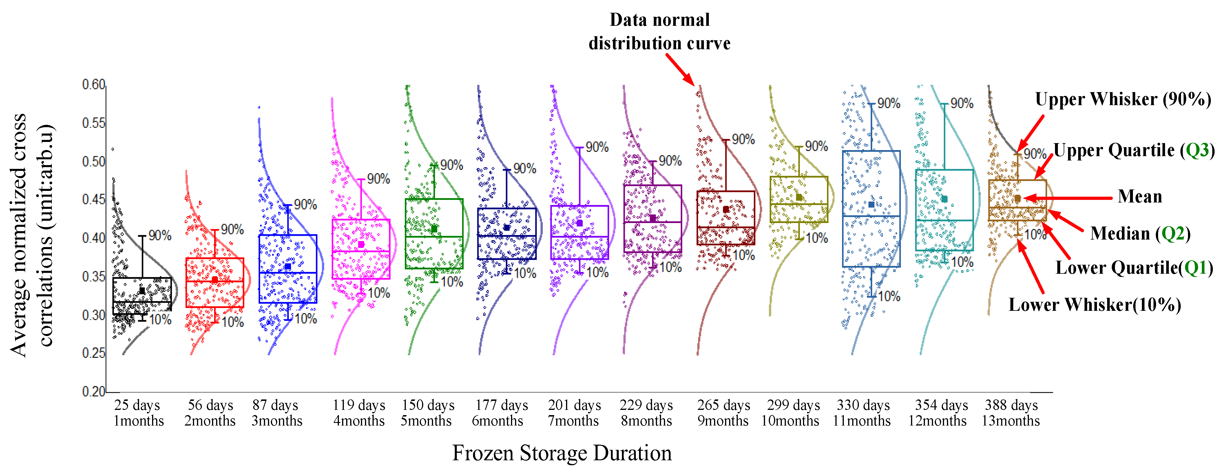
3.1. ANCC for Different Frozen Storage Durations

In this study, meat samples frozen and stored for 13 months were studied. All the samples were prepared in accordance with the method in Section 2.1 and stored under freezing conditions (−20 °C). After thawed to room temperature (about 20 °C), their pH values were firstly measured, and then using SS-OCT with a low-frequency electric field their ANCCs were measured. The detailed information is listed in

Table 1. Information of frozen meat samples.

Frozen Storage Duration		Samples after Thawing	PH Value	Temperature When Measured	Measured Sample Piece Number
Months	Days
1	25		5.33	20.1 °C	297
2	56		5.41	20.3 °C	275
3	87		5.42	20.0 °C	297
4	119		5.49	20.3 °C	297
5	150		6.04	20.1 °C	297
6	177		5.83	20.0 °C	297
7	201		5.06	20.3 °C	297
8	229		5.63	20.2 °C	297
9	265		5.69	20.3 °C	297
10	299		5.83	20.1 °C	298
11	330		5.51	20.1 °C	297
12	354		5.99	20.3 °C	297
13	388		5.94	20.0 °C	297

, and the ANCC results are plotted in Figure 3.

In statistical analysis, the box plot method as one of the useful tools has advantages such as the visual identification of outliers in a data batch [17]. Therefore, it was selected in this study to analyze the ANCC values of meat samples with different frozen storage durations. As shown in Figure 3, six important statistical parameters of the box plot were determined including the lower quartile value (Q1), the median value (Q2), the mean value, the upper quartile value (Q3), and the upper and lower Whisker values. For each meat sample, more than 200 pieces were measured, then their ANCCs were found to follow a normal distribution. Q1, Q2, Q3 and the mean value of Figure 3 are presented in

Table 2. Statistical analysis of frozen meat samples with different storage durations.

Frozen Storage Duration		Lower Quartile (Q1)	Median (Q2)	Upper Quartile (Q3)	Mean
Months	Days
1	25	0.27	0.32	0.52	0.33
2	56	0.26	0.35	0.46	0.35
3	87	0.26	0.36	0.61	0.36
4	119	0.30	0.38	0.66	0.39
5	150	0.29	0.40	0.69	0.41
6	177	0.30	0.40	0.70	0.41
7	201	0.33	0.40	0.73	0.42
8	229	0.31	0.42	0.62	0.44
9	265	0.36	0.42	0.70	0.44
10	299	0.38	0.45	0.61	0.45
11	330	0.28	0.43	0.74	0.44
12	354	0.34	0.42	0.83	0.45
13	388	0.37	0.44	0.73	0.45

.

The average state reserve time of frozen pork for different countries is 4 months. The frozen storage durations of our samples in Table 2 are from 1 month to 13 months. According to the average state reserve time, these samples are divided into three sections to quantitatively analyze the relationship between ANCC and frozen storage duration. The first section (Section 1 in Figure 4a: within 120 days) includes the frozen meat samples from 1 month to 4 months, which are within the state reserve time. Additionally, the second (Section 2: 121–240 days) and third sections (Section 3: over 240 days) are from 5 to 8 months and from 9 to 13 months. They are within twice and triple the average state reserve time, respectively. Their mean ANCC values are plotted in Figure 4a. From Table 1, 3840 samples in total were detected for different frozen storage durations. It is obvious that as the frozen storage duration increases, the ANCC mean value also clearly increases, which indicates that the ANCC value detected via SS-OCT under a low-frequency electrical field is useful for evaluation the duration of frozen meat storage.

Considering sensitivity, the growth rate for the mean ANCC value with different storage durations is discussed. Linear fitting is applied to the mean values of Section 1 to Section 3. Their slopes (labeled Slopt_n, n = 1, 2, 3) of the fitted lines are calculated. Slopt₁, Slopt₂ and Slopt₃ are equal to 6.07 × 10⁻⁴, 3.84 × 10⁻⁴ and 0.65 × 10⁻⁵, respectively. For Section 1, which is within the state reserve time, the ANCC value is quite sensitive to frozen storage duration. When the storage duration increases to twice the mean state reserve time, the ANCC growth rate drops to half of that of Section 1 which means the ANCC sensitivity to frozen storage duration is reduced by two times compared to that of Section 1. The ANCC value then increases very slowly when the storage duration is within three times the mean state reserve time, and its growth rate is only one tenth of that of Section 1. Based on this trend, Slopt₁, Slopt₂ and Slopt₃ are linearly fitted as shown in Figure 4b. It can be seen that the ANCC growth rate becomes zero when x is about 3.30. Therefore, it can be concluded that the maximum detected frozen storage duration is 396 days, which is 3.30 times the mean state reserve time (4 months).

3.2. ANCC Inversion Law for Frozen Storage Duration

Polynomial fitting has been proven to have the best fitting accuracy for all the ANCC mean values in Table 2. In this way, the ANCC inversion law for frozen meat samples for which the storage duration is within 13 months can be obtained as shown in Figure 5a. For our experiment setup, the inversion law is $y=3.19\times 10^{-4}x-2.09\times 10^{-7}{x}^2+0.33$, wherein x is the storage duration (unit: day), and y is the measured ANCC mean. The coefficient of determination (Adj. R-square) for polynomial fitting is 0.9507, and its regular residuals are shown in Figure 5b. An application program is developed to predict the frozen storage duration of pork meat within 13.2 months (396 days). Its software interface diagram is shown in Figure 6. In order to verify its accuracy, 9 pieces of meat samples under different frozen storage durations (within 4, 8 and 13 months) were investigated. In

Table 3. The accuracy analysis performed to predict the frozen storage duration via ANCC.

Sample	#1	#2	#3	#4	#5	#6	#7	#8	#9
	Within 4 Months			Within 5–8 Months			Within 9–13 Months
Ground truth (days)	28	54	120	155	199	225	279	311	368
Prediction results (days)	26.4	55.3	125.2	151.0	203.4	231.3	285.5	320.4	364.4
Absolute Error (days)	1.6	−1.3	−5.2	4.0	−4.4	−6.3	−6.5	−9.4	3.6
Relative Error	5.71%	2.40%	4.33%	2.58%	2.21%	2.80%	2.33%	3.02%	0.98%
Mean Error	4.15%			2.53%			2.11%

Note: Absolute error = ground truth − prediction results; relative error = |(absolute error/ground truth)|/100.

, the ground truths and the results predicted via the ANCC are given. The ground truths are known based on their purchase data, and the prediction results are decimals because they are calculated using the application program based on the ANCC inversion law in Figure 5. The absolute and relative errors for each sample are obtained, and the mean errors for three different frozen storage duration sections are given. It can be seen that for frozen storage durations from 0 to 13 months, all the absolute errors are less than 10 days, and their relative errors are less than 5.71%. The errors of Sample #1 to #3 within the state reserve time (4 months) are slightly larger than others, but are acceptable because their storage time is very short, and in fact the significance of predicting frozen storage within the state reserve time is not great. For Sample #4 to #6 and Sample #7 to #9, the storage durations are two and three times the state reserve time. Their absolute errors are also less than 10 days, and the relative errors are less than 3.02%, which potentially proves that the SS-OCT detection method using a low-frequency electric field has the ability to accurately predict storage durations in days for frozen meat samples exceeding the state reserve time by three times.

4. Discussion

4.1. ANCC and Biological Characteristics

It has been reported the metmyoglobin in pork changes under different frozen storage durations (from 12 to 24 weeks, −18 °C) [18]. According to this research result, an increase in ANCC with frozen storage duration may be related to the metmyoglobin content change. Secondly, the impedance of chicken breast muscles frozen for over 8 months has been reported to decrease, and has close relationship with PH, color, water holding capacity, lipid oxidation and protein solubility [19]. The decreasing impedance may therefore make samples more sensitive to the applied AC current, and then lead to the visible vibrations in SS-OCT detections. This could be thought of as another reason that causes an increase in ANCC. Fresh meat is rich in water with little loss via dripping. When it is frozen rapidly under −20 degrees, uneven changes in its biological structure may lead to large differences in the refractive index distribution. When a low-frequency electric field is turned on, uneven compositions vibrate irregularly, and the difference in ANCC for a short duration of freezing meat is large. With the increase in the frozen storage duration, the loss of water, muscle fiber tissue atrophy and other factors both on the surface and inside samples make the changes in refractive index have a tendency to be balanced. Therefore, the growth rate of ANCC becomes slow.

4.2. ANCC Influencing Factor

In theory, ANCC values between two adjacent SS-OCT images should be the same for a sample without a low-frequency electric field because without a electro-kinetic response there should be no change in SS-OCT images. In order to determine whether or not there are some other factors that may affect the ANCC value, SS-OCT images without applying a low-frequency electric field are analyzed. The electric-kinetic properties of meat are obvious in the ROI, which is expected to have the best contrast and axial resolution. According to the principle of optical coherence tomography, contrast and axial resolution depend on the optical path difference between the reference beam (the reflected light from the reference mirror) and the sample beam (rgw scattered light from the sample) as shown in Figure 1. As shown in Figure 7, the main parameters that affect the optical path difference are d and z. d is the distance between the sample’s surface and Needle A. z is the sample’s distance from the surface in the SS-OCT image’s field of view. The distance, d, changes by a little because the meat sample and Needle A are fixed by the sample holder. Therefore, z should be mainly considered. SS-OCT images of meat samples of which the surfaces are in different imaging positions (z = 0.05 mm to 1.35 mm) along the vertical direction are collected as shown in Figure 7. Due to Needle B being out of the field of view, only Needle A can be observed in Figure 7. Sample surface is the bright curve in each subgraph (a)–(h) in Figure 7 which is also the boundary between the air and meat sample. As shown in Figure 7h, the distance between the upper and lower limit of the bright curve is labeled $\mathsf{\Delta }$. We define the surface center as the blue line located in the middle of the upper and lower limit ($\frac{\mathsf{\Delta }}{2}$). z is defined as the distance from the top of the image to the surface’s center. As shown in Figure 7, with the changes in z from 0.05 mm to 0.8 mm the axial resolution and the contrast of the ROI change. In order to analyze this quantitatively, the contrasts in the ROI are calculated and shown in Figure 8. The point with the maximum contrast inside the ROI is found for each subgraph. Passing through this point, Line A is plotted as shown in Figure 8 to discuss its contrast distribution with the changes in z. The full widths at half maximum (FWHM) are then calculated and labeled in Figure 8. It can be seen in our experiments that when z equals 1.0, there is the maximum contrast and the minimum FWHM which means that under this condition the best SS-OCT axial resolution for the ROI can be obtained. For the ROI with a different contrast and axial resolution, the ANCC value changes a lot. As shown in Figure 9, with the increase in z the ANCC value first decreases and then increases. When z = 1.0 mm, ANCC reaches the minimum where the axial resolution and the contrast in the ROI are the best. Under this condition, the randomness of noise (such as thermal noise) is not so obvious due to the high signal-to-noise ratio which makes each SS-OCT image during one measurement without a low-frequency electric field very similar to the others. Therefore, it is necessary to place the ROI at a suitable z position. In this way, the good axial resolution and contrast inside the ROI can be achieved to study the ANCC of meat with different frozen durations well.

The distance d and z are along the scattered sample beam. d is the distance between sample’s surface and Needle A. z is the sample’s surface distance in SS-OCT image field of view. The meat sample and Needle A are fixed by the sample holder in Figure 1, so the change for d value is very small. In Figure 7a–h, z values different from 0.05 mm to 1.35 mm are discussed for the contrast and axial resolution for ROI. When z = 1.0 mm the axial resolution and the contrast of ROI are the best. Under this condition, the randomness of noise (such as thermal noise) is not so obvious due to the high signal to noise ratio which makes each SS-OCT image during one measurement without low frequency electric field very similar.

5. Conclusions

In this paper, we report an optical detection method via SS-OCT under a low-frequency electric field for predicting the storage duration of frozen meat which may have exceeded the state reserve time (4 months) by two or three times. The internal electro-kinetic response of the meat sample is visualized, and the parameter ANCC is developed and then proven to be sensitive to different frozen storage durations. A steadily increasing relationship between the ANCC and frozen storage duration is found. The growth rate of the ANCC is analyzed in detail, and the maximum frozen storage duration is therefore concluded. Finally, the ANCC inversion law for different storage duration is established. To verify the inversion law, samples within and exceeding the state reserve time by two and three times are investigated. The experimental results show that the absolute errors for all samples are less than 10 days, and the relative errors are below 5.71%, which proves that our inversion law has a good capability to predict frozen meat storage durations. To the best of our knowledge, we are the first to predict frozen meat storage durations via SS-OCT under a low-frequency electric field. Although pork, as the largest national reserve meat, is our current research object, SS-OCT under a low-frequency electric field should be applied to other kinds of meat products, such as beef and chicken. Related research will be carried out in the near future. In conclusion, with the help of the ANCC, SS-OCT under a low-frequency electric field has the potential to provide a novel rapid detection method without complex physical and chemical operations for food safety inspection.

References

1. Zhang, L.; Zhang, M.; Mujumdar, A.S. Technological innovations or advancement in detecting frozen and thawed meat quality: A review. Crit. Rev. Food Sci. 2021, 63, 1–17. [Google Scholar] [CrossRef] [PubMed]
2. Sabikun, N.; Bakhsh, A.; Ismail, I.; Hwang, Y.H.; Rahman, M.S.; Joo, S.T. Changes in physicochemical characteristics and oxidative stability of pre- and post-rigor frozen chicken muscles during cold storage. JFST 2019, 56, 4809–4816. [Google Scholar] [CrossRef] [PubMed]
3. Muela, E.; Monge, P.; Sanudo, C.; Campo, M.M.; Beltrán, J.A. Meat quality of lamb frozen stored up to 21 months: Instrumental analyses on thawed meat during display. Meat Sci. 2015, 102, 35–40. [Google Scholar] [CrossRef] [PubMed]
4. Byun, J.S.; Min, J.S.; Kim, I.S.; Kim, J.W.; Chung, M.S.; Lee, M. Comparison of indicators of microbial quality of meat during aerobic cold storage. J. Food Prot. 2003, 66, 1733–1737. [Google Scholar] [CrossRef] [PubMed]
5. Xie, A.; Sun, D.W.; Zhu, Z.; Pu, H. Nondestructive Measurements of Freezing Parameters of Frozen Porcine Meat by NIR Hyperspectral Imaging. Food Bioprocess Technol. 2016, 9, 1444–1454. [Google Scholar] [CrossRef]
6. Xie, A.; Sun, D.W.; Xu, Z.; Zhu, Z. Rapid detection of frozen pork quality without thawing by Vis–NIR hyperspectral imaging technique. Talanta 2015, 139, 208–215. [Google Scholar] [CrossRef] [PubMed]
7. Ma, J.; Sun, D.W.; Pu, H.; Wei, Q.; Wang, X. Protein content evaluation of processed pork meats based on a novel single shot (snapshot) hyperspectral imaging sensor. J. Food Eng. 2019, 240, 207–213. [Google Scholar] [CrossRef]
8. Leitgeb, R.; Hitzenberger, C.K.; Fercher, A.F. Performance of Fourier domain vs. time domain optical coherence tomography. Opt. Express 2003, 11, 889–894. [Google Scholar] [CrossRef] [PubMed]
9. Thampi, A.; Hitchman, S.; Coen, S.; Vanholsbeeck, F. Towards real time assessment of intramuscular fat content in meat using optical fiber-based optical coherence tomography. Meat Sci. 2021, 181, 108411. [Google Scholar] [CrossRef] [PubMed]
10. Pena, A.; Sadovoy, A.; Doronin, A.; Bykov, A.; Meglinski, I. Evaluation of freshness of soft tissue samples with optical coherence tomography assisted by low frequency electric field. Sovrem. Tehnol. 2015, 7, 69–74. [Google Scholar] [CrossRef]
11. Thampi, A.; Hitchman, S.; Coen, S.; Vanholsbeeck, F. Optical coherence tomography to predict the quality of meat. In Optical Coherence Imaging Techniques and Imaging in Scattering Media III; SPIE: Bellingham, WA, USA, 2019; p. 11078. [Google Scholar]
12. Trabelsi, S. Measuring changes in radio-frequency dielectric properties of chicken meat during storage. J. Food Meas Charact 2018, 12, 683–690. [Google Scholar] [CrossRef]
13. Youn, J.I.; Akkin, T.; Milner, T.E. Electrokinetic measurement of cartilage using differential phase optical coherence tomography. Physiol. Meas. 2004, 25, 85–95. [Google Scholar] [CrossRef] [PubMed]
14. Jia, P.; Zhao, H.; Qin, Y. Laser Lens Size Measurement Using Swept-Source Optical Coherence Tomography. Appl. Sci. 2020, 10, 4936. [Google Scholar] [CrossRef]
15. Gonzalez, R.C.; Woods, R.E.; Masters, B.R. Digital Image Processing, Third Edition. J. Biomed Opt. 2009, 14, 029901. [Google Scholar] [CrossRef]
16. Lim, J.S. Two-Dimensional Signal. and Image Processing; Prentice Hall: Englewood Cliffs, NJ, USA, 1990; p. 548. [Google Scholar]
17. Benjamini, Y. Opening the box of a boxplot. TAS 1988, 42, 257–262. [Google Scholar]
18. Teuteberg, V.; Kluth, I.K.; Ploetz, M.; Krischek, C. Effects of duration and temperature of frozen storage on the quality and food safety characteristics of pork after thawing and after storage under modified atmosphere. Meat Sci. 2020, 174, 108419. [Google Scholar] [CrossRef] [PubMed]
19. Wei, R.; Wang, P.; Han, M.; Chen, T.; Xu, X.; Zhou, G. Effect of freezing on electrical properties and quality of thawed chicken breast meat. AJAS 2016, 30, 569–575. [Google Scholar] [CrossRef] [PubMed]
Figure 1. Schematic diagram of our SS-OCT experimental system.
Photonics 10 00956 g001
Figure 2. Average normalized cross-correlation algorithm. (a) SS-OCT image collection. (b) Wiener filtering. (c) Normalized cross-correlation calculation for specific line in SS-OCT image. (d) Region of interest (ROI) selection. (e) Normalized cross-correlation map. (f) Average normalized cross-correlation (ANCC) curve.
Photonics 10 00956 g002
Figure 3. Average normalized cross-correlation (ANCC) analysis of samples with different frozen storage durations using the box plot method.
Photonics 10 00956 g003
Figure 4. The growth rate analysis of the ANCC mean. (a) ANCC growth rate analysis. (b) The maximum frozen storage duration.
Photonics 10 00956 g004
Figure 5. ANCC inversion law for frozen storage duration. (a) ANCC inversion law. (b) Error analysis for ANCC inversion law.
Photonics 10 00956 g005
Figure 6. Our developed software interface for frozen storage duration prediction.
Photonics 10 00956 g006
Figure 7. Different positions of meat sample surface in vertical direction.
Photonics 10 00956 g007
Figure 8. Quantitively analysis of the influence of the z value. The maximum contrast in the ROI is determined. Passing through the point with the maximum normalized intensity, a perpendicular line (Line A) is drawn. The contrast values on Line A are plotted for SS-OCT images with different z values. The full widths at half maximum (FWHM) are measured. When z equals 1.0, there is the maximum contrast and the minimum FWHM.
Photonics 10 00956 g008
Figure 9. ANCC for different sample surface positions, z, without a low-frequency electrical field. ANCC reaches the minimum when z = 1.0 mm, where the axial resolution and the contrast in the ROI are the best. The reason may be that under this condition, the randomness of noise is not so obvious due to the high signal-to-noise ratio. Hence, each SS-OCT image during a measurement without a low-frequency electric field is similar to the others, which makes the ANCC the minimum.
Photonics 10 00956 g009