Fiber-Optic Hydraulic Sensor Based on an End-Face Fabry–Perot Interferometer with an Open Cavity

Abstract

The paper describes the design and manufacturing process of a fiber optic microphone based on a macro cavity at the end face of an optical fiber. The study explores the step-by-step fabrication of a droplet-shaped macro cavity on the optical fiber’s end surface, derived from the formation of a quasi-periodic array of micro-cavities due to the fuse effect. Immersing the end face of an optical fiber with a macro cavity in liquid leads to the formation of a closed area of gas where interfacial surfaces act as Fabry–Perot mirrors. The study demonstrates that the macro cavity can act as a standard foundational element for diverse fiber optic sensors, using the droplet-shaped end-face cavity as a primary sensor element. An evaluation of the macro cavity interferometer’s sensitivity to length alterations is presented, highlighting its substantial promise for use in precise fiber optic measurements. However, potential limitations and further research directions include investigating the influence of external factors on microphone sensitivity and long-term stability. This approach not only significantly contributes to optical measurement techniques but also underscores the necessity for the continued exploration of the parameters influencing device performance.

1. Introduction

Fiber-optic sensors have gained significant popularity in various fields of science and technology due to their unique properties, such as immunity to electromagnetic interference, small size, light weight, high sensitivity, and the absence of sensor power supply. At present, a wide range of technical solutions has been proposed in the development of interferometric fiber-optic sensors, which are used for measuring temperature, deformation, pressure, refractive index, acoustic waves, vibration, stress, current strength, magnetic field, and more. The most common types of interferometric fiber-optic sensors include Fabry–Perot, Michelson, Mach–Zehnder, Sagnac, and others. Compared to other types of fiber-optic interferometers, sensors based on the Fabry–Perot interferometer (FPI) [1] offer advantages such as compactness, and the simplicity of its design and manufacturing. There are two main categories of Fabry–Perot fiber-optic interferometers: internal and external, both of which can be implemented in various configurations. Intrinsic Fabry–Perot interferometers are formed inside the optical fiber between two coaxial fiber reflectors [2]. External Fabry–Perot cavities are formed between the end face of the cleaved fiber and an external reflector. The external resonator on the FPI can be solid, filled with air (gas), or liquid, with an external reflector made of thin film or formed as a boundary between the resonator medium and the surrounding environment [3]. In this work, we focus on the development of an external fiber-optic Fabry–Perot interferometer (FPI) for detecting acoustic waves in liquids. Firstly, we examined the current state of related applications of FPI, specifically hydrostatic pressure measurements. Two directions of development can be distinguished for pressure sensors based on FPI: first, the development of sensors with enhanced sensitivity, and second, the development of sensors designed for adverse operating conditions. There are numerous factors influencing the metrological characteristics of pressure sensors based on FPI, among which the characteristics of the diaphragm (material properties, thickness, diameter) are most significant. Quartz glass is of interest as a diaphragm material due to its chemical resistance and thermal expansion coefficient, which are similar to optical fiber [4,5]. In [6], a sensor based on a diaphragm made of quartz glass, formed from a cleaved multimode fiber attached to a capillary, is presented. The FPI based on a diaphragm made of fused quartz with a thickness of 30 μm demonstrated a sensitivity of 5.3 nm/kPa [7]. However, the fabrication of ultra-thin (sub-micron) membranes is associated with technological challenges, limiting the sensitivity of such sensors. Nevertheless, in [8], an FPI with a diaphragm thickness of 170 nm and spectral sensitivity of 12.22 nm/kPa was demonstrated. In addition to quartz glass, various polymer materials such as polyurethane and polystyrene are used for the fabrication of fiber-optic FPI membranes. For instance, in [9], an FPI with a sensitivity of 3.33 nm/kPa is presented. A common drawback of polymer materials is the need for their pre-stabilization. There are numerous alternative approaches to manufacturing flexible FPI membranes from other materials: silver [10], graphene [11], fibroin [12], PDMS [13,14], silicone rubber [15], two-component epoxy adhesive film [16], and steel [17]. The spectral sensitivity of the mentioned examples of FPI varies from 0.2 to several nm/kPa. The maximum operating temperature of sensors manufactured using the aforementioned technologies does not exceed 100 °C due to the difference in thermal expansion coefficients between the membrane and the optical fiber. Therefore, for the creation of pressure sensors operating at elevated temperatures, it is preferable to create all-glass sensing elements [18]. In many cases, the FPI resonator is formed by welding a fiber with a hollow core and cleaving a single-mode optical fiber; in addition, liquid etching is applied to the the cleaved multi-mode fiber [9], along with three-dimensional microprinting [19] and focused ion beam micro-processing [20]. An alternative approach to manufacturing the FPI resonator was proposed, using the catastrophic destruction (melting) effect of a single-mode fiber with a powerful source [21]. As a result of this effect, multiple periodic voids are formed in the fiber core with a period of several micrometers. To obtain the resonator, such a fiber is cleaved and spliced with an undamaged single-mode fiber, resulting in the formation of a drop-like cavity about a hundred microns long at the joint, forming a Fabry–Perot interferometer. Such a cavity, cleaved at the narrowing end, can serve as a diaphragm-less pressure sensor. The liquid–gas interfacial boundary in this case acts as an external reflector. The FPI obtained in [21] has a sensitivity of about 0.5 nm/kPa, which is comparable to the above-mentioned membrane-based sensitive elements. In [22], a similar FPI, which is enclosed with a polyurethane diaphragm, was obtained by welding a cleaved fiber with a cavity to a single-mode fiber. The claimed pressure sensor sensitivity was 0.45 nm/kPa.

When designing and operating pressure sensors based on FPI, it is necessary to consider their cross-sensitivity to temperature, arising from the thermal expansion of FPI components. To account for the temperature drift in the spectral characteristics of FPI, using an isolated fiber Bragg grating (FBG) located near the FPI has been proposed, serving as a temperature sensor [23,24,25]. In this case, the shift in the central wavelength of the FBG is used to compensate for the temperature-induced shift in the FPI spectrum.

Another direction of development for external fiber-optic FPIs is acoustic (infrasound) detection and photoacoustic detection. In most cases, an acoustic sensor based on an external FPI consists of a flat end face optical fiber and an acoustically sensitive Fabry–Perot resonator, which is usually in the form of a thin membrane or cantilever. Membrane-based acoustic FPI sensors utilize the deflection of the membrane caused by external pressure induced by an acoustic wave. These sensors can be divided into three types depending on the material used for membrane fabrication: polymer-based, metal-based, and 2D material-based (a crystal consisting of one or several layers where intraplanar atomic interactions are much stronger than interplanar ones). Polymer-based sensors usually have higher sensitivity compared to metal-based sensors due to the significantly lower Young’s modulus of polymer materials [26]. For instance, a sensor with a polyimide membrane with a sensitivity of 2239 nm/Pa was proposed in [27]. To enhance the sensitivity of metal-based sensors, it is necessary to reduce the thickness of the metal membrane, which can be achieved through the “silver mirror” reaction [28] (a reaction involving the reduction of silver from an ammoniacal solution of silver oxide), resulting in a structure with a sensitivity of 160 nm/Pa, or by using electron beam evaporation techniques [29]. Composite membrane structures have also been proposed, such as a polyethylene terephthalate film with a thin layer of aluminum foil [30]. Another approach to constructing a metal-based sensor with enhanced sensitivity involves using a corrugated silver membrane [31], resulting in a sensitivity of over 80 nm/Pa. Two-dimensional (2D) materials also attract significant interest in the design of acoustic sensors due to their small thickness and mechanical properties. An external FPI made of a graphene membrane can have a wideband frequency response from infrasound to 20 kHz [32,33]. Micro-electromechanical systems (MEMS) technology is also employed in the fabrication of highly sensitive acoustic FPI sensors. It is reported that a sensor with a cantilever on a silicon membrane has a sensitivity of 1.753 μm/Pa at a frequency of 1 kHz [34].

The current work focuses on two main points. The first one is the development of the technological process and the creation of an open drop-shaped cavity at the end of the optical fiber, similar to [35], elaborating on the repeatability of the cavity shape and the factors that influence it. The second one is a theoretical and practical study of the possibility of using an open drop-shaped cavity at the end of an optical fiber as a membrane-less Fabry–Perot interferometer acting as an acoustic sensor that allows monitoring sound vibrations propagated in a liquid medium.

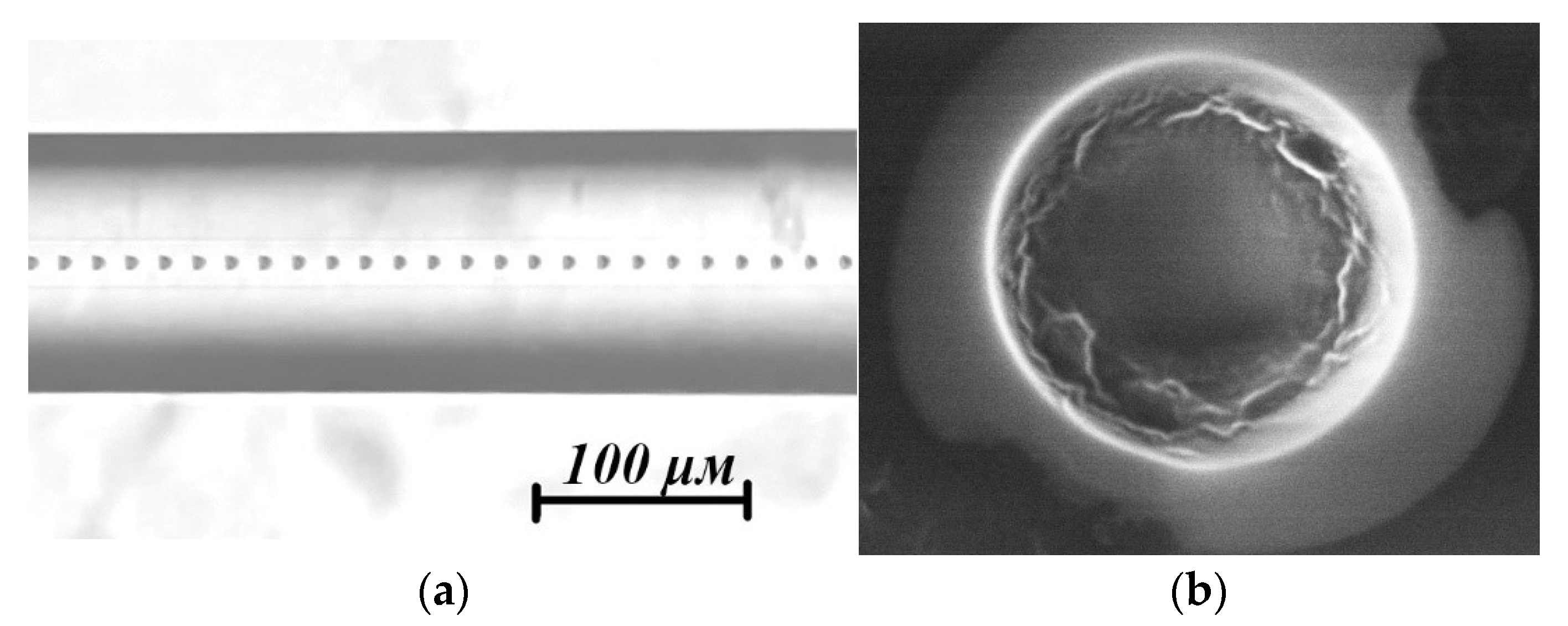
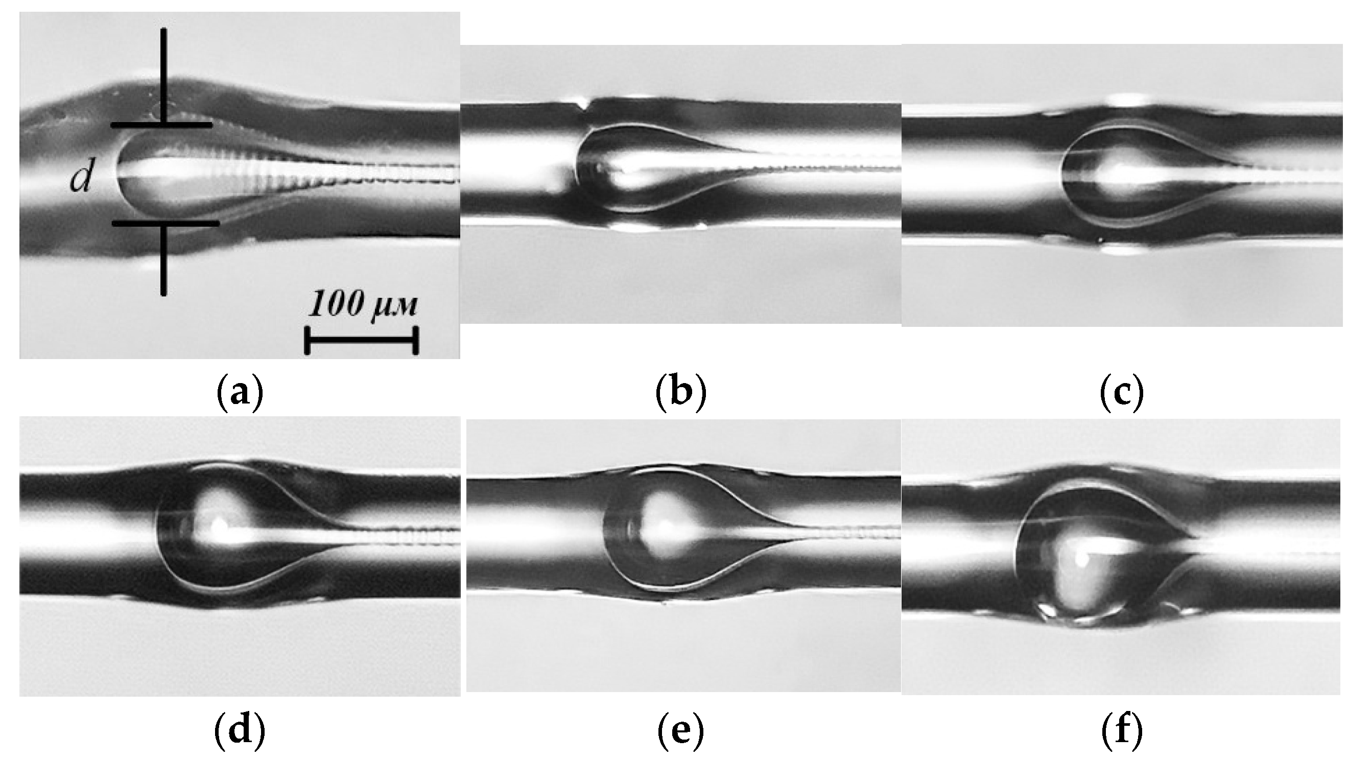
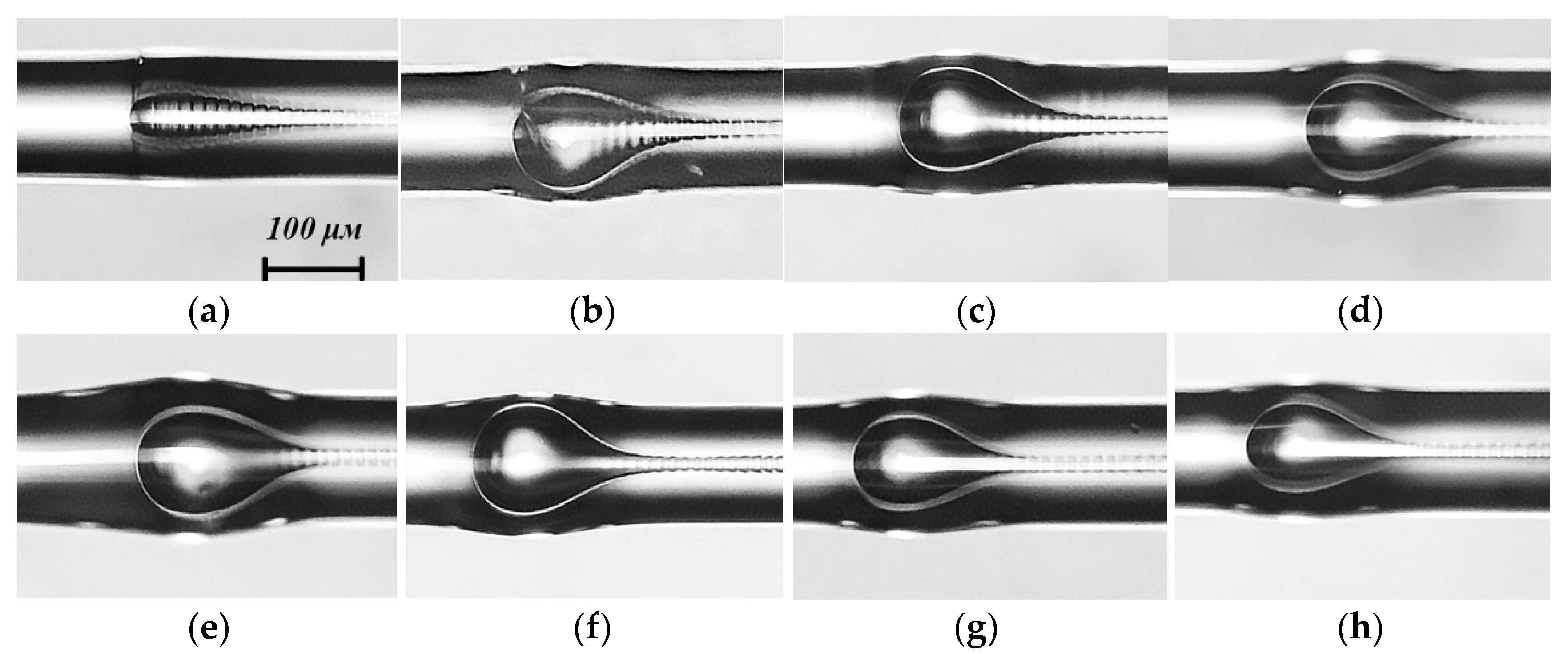
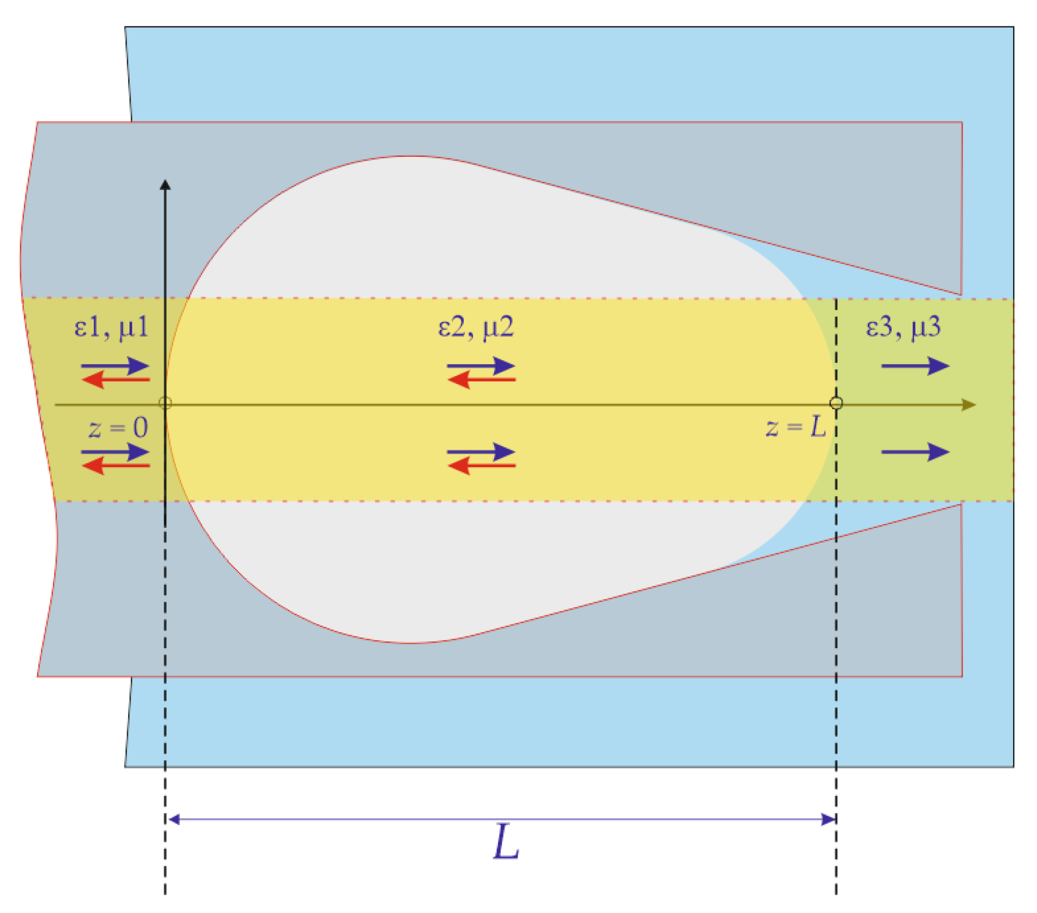
2. Open Cavity Formation at the End Face of an Optical Fiber

The creation of an open cavity in the form of a droplet on the end face of an optical fiber proceeds through several stages.

In the first stage, inside the optical fiber (SMF-28), a quasi-periodic array of micro-cavities is generated through the effect of catastrophic plasma melting [35,36] (Figure 1a). This phenomenon is accompanied by self-induced core destruction, caused by local plasma heating, which creates a locally high-temperature region propagating towards the radiation source, vaporizing the core [37]. Destruction of the optical fiber core renders it unsuitable for use in data transmission systems due to the emergence of a quasi-periodic sequence of voids with dimensions and spatial period on the order of micrometers [38,39], leading to a significant increase in optical losses. However, such structures can be utilized as standalone elements or blanks in fiber optic sensor systems.

To create micro-cavities inside the optical fiber, optical radiation from a laser (YFL-1100) with an optical power of 2 W and a wavelength of 1080 nm is used. Plasma heating is initiated by putting the end face of the optical fiber into contact with a darkened surface; for example, with black-colored ABS plastic [40]. A plasma cluster forms on the end face of the fiber, which moves back along the core, creating micro cavities. In [41], it is shown that the resulting micro-cavities are filled with oxygen at pressures ranging from 4 to 8 atmospheres.

The periodicity of the voids is associated with the cooling and stratification of the plasma (burning of the plasma followed by melting and cooling of the material, which forms layers of different composition around the bubble). In Figure 1b, a photo of the structure of the inner surface of the micro-cavity obtained with the Tescan Vega 3 scanning electron microscope is shown. It can be observed that the surface is lined with a collection of irregularities with a relatively small pitch.

At the second stage of production, a fragment of the SMF-28 optical fiber containing the end part of the micro-cavity series is cleaved and fused with an undamaged single-mode SMF-28 fiber. The electric arc softens the quartz glass, and the gas inside the micro-cavities expands. This leads to the merging of several micro-cavities into one chamber with a diameter ranging from 30 to 100 μm (Figure 2). The fusion is performed using a fusion splicer, for example, the “Inno View5”. To accurately determine the boundaries of the blank, the end-face alignment is performed based on its shell.

Variation in current strength and arc burning duration, as well as the number of micro-cavities in the blank, allows us to adjust the diameter and shape of the macro-cavity. Figure 2 shows photographs of cavities that were obtained with a Zeiss Axiovert 40 MAT microscope after the manufacture of cavities at a fixed time of contact of the discharge arc with welding elements with varying power P. The fiber was welded to the diffuser with a two-second exposure. The P value is given relative to its peak value P₀ = 1.5 W. Experiments have shown that, under equal manufacturing conditions, there is a 5% spread in the maximum transverse cavity size d. Data averaging was carried out based on the dimensions of the cavities obtained in five implementations with fixed welding parameters. As can be observed, with increasing discharge arc power, the maximum transverse cavity size d increases, already reaching a plateau at values P = 0.3∙P₀. The cavity reaches its largest size under a three-second exposure to a discharge arc at P = 0.2∙P₀.

Figure 3 shows photographs of cavities with the maximum transverse cavity size d, manufactured at a constant arc discharge power P = 0.2∙P₀ with different duration of exposure time. Thus, using the data obtained, it is possible to select the optimal mode P and t for the manufacture of cavities of a given size. In the future, a series of experiments that will make it possible to construct a complete map of modes are planned.

Using a fiber optic cleaver, an indicator laser, and an optical microscope, a section of the fiber is removed, creating an open droplet-shaped cavity at the end of the fiber (Figure 4a).

To visualize the internal volume of the cavity and liquid around the fiber, the fiber end with the sensitive element 1 was immersed in a Helle-Shaw cell 2 filled with distilled water and isopropyl alcohol, taken at a temperature of 23 ± 0.5 °C (Figure 5). Visualization was carried out using digital camera 3 interfaced with PC 7. The lens of the camera was aimed at the wide edge of the cell.

The detection of the optical signal was carried out using the setup presented in Figure 5. Laser radiation from a broadband source 4 (wavelength 1525–1570 nm, half-width 0.16 nm with a power of up to 5 mW) through port 1 and 2 of circulator 5 was directed into the fiber with the cavity under study. The circulator made it possible to simultaneously send a signal through the fiber and record the reflection spectrum through port 3 using an EXFO OSA20 6 spectrometer.

Immersing the end of the optical fiber into a liquid media leads to the formation of a closed gas bubble inside the cavity (Figure 4a) where the interface of the bubble serves as one of the mirrors in the Fabry–Perot interferometer. The other mirror in the interferometer is the boundary between the core of the optical fiber and the gas inclusion. Laser radiation directed at such a structure forms a comb-like wavelength reflection spectrum, the period and contrast of which depend on the geometric and physical characteristics, namely: the refractive index of the core of the optical fiber enclosed inside the gas cavity and the external liquid, as well as the length of the interferometer (Figure 4b).

The data shown in Figure 4b correspond to the reflection spectrum obtained when the end of the fiber was in the air (black line) and when the cavity was immersed in the liquids under study (red line—isopropanol; blue line—water) in the first minute of contact between the sensor and the medium. The graph shows that the interference signal in isopropanol has a shorter period compared to the spectrum detected in water. At the same time, a more intense flow of isopropanol into the internal volume of the cavity was observed, which led to a decrease in the size of the gas inclusion and, as a consequence, a change in the length of the Fabry–Perot interferometer. It is clear that, in addition to capillary effects, the presence of two phases in the system leads the diffusion and solubility of gas into the environment. It is known that the solubility coefficient of oxygen in water is 0.0279 at a temperature of 25 °C and normal atmospheric pressure [42]. While the solubility coefficient of oxygen in alcohols can exceed this value by orders of magnitude. Due to the above, it was decided to limit the experiments on detecting the acoustic signal to the aqueous medium, since the processes observed in isopropanol require more detailed study.

3. Mathematical Model of the Sensor

Consider an axisymmetric cavity formed at the end of an optical fiber (Figure 6a) immersed in a container with liquid. When the end of the open cavity is immersed into the liquid, a certain amount of gas is confined inside the cavity; the pressure inside of which is balanced by the liquid pressure near the fiber end. The geometry of the resulting structure is schematically depicted in Figure 6b.

Let us define the volume of the cavity as the volume of the figure of rotation formed by a part of the circle between points A and B and a fragment of the line between points B and C, rotating around the symmetry axis AD, Figure 6b. Point B is the point of tangency between the line and the circle.

Let us determine the volume of the cavity by relying on three of its basic dimensions as a body of rotation that can be readily measured: the radius of the spherical part of the cavity—OB (R); the total length of the cavity—AD (H); and the radius of the exit hole—CD (r). Let us represent the volume of the body of rotation as the sum of the volumes of a truncated sphere obtained by rotating arc AB around AE and a truncated cone obtained by rotating straight line BC around ED. After elementary mathematical transformations, we obtain the final ratio that defines the volume of the figure of rotation by its three measured parameters—the radius of the spherical part (R); the radius of the exit hole (r); and the total height (H):

$$V_0=\frac{4\pi }{3}{R}^3-\frac{\pi }{6}\left(R-b\right)\left(3d^2+{\left(R-b\right)}^2\right)+\frac{\pi }{3}\left(h-b\right)\left(r^2+rd+d^2\right)\hspace{0.33em},$$

(1)

where d and b are defined according to Equation (2).

$$d= R\frac{\left(H-R\right)\sqrt{r^2-2HR+H^2}+Rr}{r^2+{\left(H-R\right)}^2}\hspace{0.33em}, b=\frac{R}{\sqrt{r^2+h^2-R^2}}\left(d-r\right).$$

(2)

After the fabrication of the cavity, its geometry does not change, which allows us to define the volume of the cavity as V₀ = V(r, R, H) = const.

The relationship between the pressure, temperature, and volume of air (or other ideal gas) in a cavity can be described by the Clapeyron–Mendeleev equation:

$$\frac{PV}{T}=\frac{m}{M}\Re ,$$

(3)

which relates the pressure P, volume V, and temperature T of a gas to the molar mass M and mass m; ℜ is the universal gas constant.

The equation of state (3) for a given pressure P₀ and temperature T₀ allows us to determine the mass of gas that completely fills the cavity:

$$m=\frac{P_0{V}_0}{T_0}\frac{M}{\Re }.$$

(4)

The equation of state (3) with a known gas mass m allows us to describe the change in the volume of the gas initially filling the cavity completely when a drop-shaped macro-cavity is immersed in liquid. The pressure inside the gas P, including ΔP = 2σ/q, over the pressure determined by surface tension forces (q—radius of curvature of the surface), is balanced by the pressure in the liquid column:

$$P+\frac{2\sigma }{q}=\rho gh,$$

(5)

where h is the liquid column height, and ρ ii is the liquid density.

The gas pressure P at temperature T determines its volume V (3). On the other hand, the volume of the gas is equal to the difference in the volumes of the whole cavity and the liquid flowing into the cavity:

$$V=V_0-V_{\mathrm{L}}.$$

(6)

The volume of liquid V_L flowing into the cavity can be written as the difference in the volumes of a truncated cone of height SD with radii s = |ST|, r = |CD| and a spherical segment of a sphere of radius q = |QT| with height |SP| = q − t and base radius s = |ST|, which allows us to write an expression for the volume of gas:

$$V=V_0-\frac{\pi }{3}\frac{{\left(H-L\right)}^3}{{\left(H-2R\right)}^3}\left(\left(H-R-b\right)\left(d^2+dr\frac{H-2R}{H-L}+r^2{\left(\frac{H-2R}{H-L}\right)}^2\right)-\frac{R-b}{2}\left(3d^2+{\left(R-b\right)}^2\right)\right)$$

(7)

With a high degree of accuracy, if the temperature in the liquid coincides with the temperature in the gas, T = T_L = T_G, we obtain an equation relating the linear size of the air droplet L with the geometric dimensions of the cavity, as well as with the density of the liquid, the height of the liquid column, and temperature:

$$\frac{P}{T}\left(V_0-\frac{\pi }{3}{\left(\frac{H-L}{H-2R}\right)}^3\left(\begin{array}{l}\left(H-R-b\right)\left(d^2+dr\frac{H-2R}{H-L}+r^2{\left(\frac{H-2R}{H-L}\right)}^2\right)-\\ -\frac{R-b}{2}\left(3d^2+{\left(R-b\right)}^2\right)\end{array}\right)\right)-\frac{m}{M}\Re =0.$$

(8)

The expression we obtained allows us to relate the distance L between the two mirror surfaces forming the Fabry–Perot interferometer to the temperature and immersion depth of the drop-shaped macro cavity.

The Fabry–Perot reflection coefficient additionally depends on the wavelength of the radiation and the properties of the three media forming the interferometer, namely their dielectric and magnetic permeability.

Let us determine the reflection coefficient of the Fabry–Perot interferometer at each wavelength by making a system of equations ensuring the continuity of propagation of a plane electromagnetic wave through it. Let us accept the simplification of the mathematical model, consisting of the fact that light propagates only along the central axis, and the electric and magnetic field at each of its points is the sum of waves propagating in the forward and backward directions, Figure 7.

The variables are defined as follows: t_i is the transmission coefficient; r_i is the reflection coefficient; k_i is the wave number, w_i is the wave impedance; 1 is the layer of optical fiber core; 2 is the layer with gas; 3 is the layer with liquid; the absolutely absorbing medium is at infinity; index i defines the layer number. Wave number and wave impedance are defined as:

$${\mathsf{\kappa }}_i=\frac{\sqrt{{\mathsf{\epsilon }}_i{\mathsf{\mu }}_i}}{\mathsf{\lambda }},\hspace{0.33em}{w}_i=\sqrt{\frac{{\mathsf{\mu }}_0{\mathsf{\mu }}_i}{{\mathsf{\epsilon }}_0{\mathsf{\epsilon }}_i}},$$

(9)

where ε_i is the relative dielectric permittivity, μ_i is the relative magnetic permeability of the substance, λ is the wavelength of radiation, ε₀ is the permittivity, and μ₀ is the permeability of free space.

The equations for the electric and magnetic fields are of the form:

$$E_i(z)=t_i\cdot {\mathrm{e}}^{-j{\mathsf{\kappa }}_{i}z}+r_i\cdot {\mathrm{e}}^{j{\mathsf{\kappa }}_{i}z},H_i(z)=\frac{1}{w_i}\left(t_i\cdot {\mathrm{e}}^{-j{\mathsf{\kappa }}_{i}z}-r_i\cdot {\mathrm{e}}^{j{\mathsf{\kappa }}_{i}z}\right).$$

(10)

Let us write down the conditions determining the continuity of propagation in the electric and magnetic waves, which consists of the equality of these fields at each of the boundaries of the medium interfaces at z = 0 and at z = L. We consider that all the radiation that approached the boundary z = 0 entirely falls on it (t₁ = 1), and all the radiation that passed through the boundary z = L is not reflected back (r₃ = 0). We obtain a complete system of four linear equations with respect to four unknown variables r₁, t₂, r₂, t₃; the reflection and transmission coefficients are [43]:

$$\left[\begin{array}{cccc}1& -1& -1& 0\\ -w_2& -w_1& w_1& 0\\ 0& {\mathrm{e}}^{-j{\kappa }_{2}L}& {\mathrm{e}}^{j{\kappa }_{2}L}& -{\mathrm{e}}^{-j{\kappa }_{3}L}\\ 0& w_3{\mathrm{e}}^{-j{\kappa }_{2}L}& -w_3{\mathrm{e}}^{j{\kappa }_{2}L}& -w_2\cdot {\mathrm{e}}^{-j{\kappa }_{3}L}\end{array}\right]\times \left[\begin{array}{c}{r}_1\\ t_2\\ r_2\\ t_3\end{array}\right]=\left[\begin{array}{c}-1\\ -w_2\\ 0\\ 0\end{array}\right].$$

(11)

The coefficient r₁ describes the reflection of an electromagnetic wave traveling in the opposite direction. Let us reduce (11) to the lower triangular form and obtain the dependence of the reflection coefficient on the length L of the Fabry–Perot interferometer, determined by solving Equation (8), and the permittivity and permeability of the layers:

$$r_1={\left|\frac{\cos \left(2\pi \sqrt{{\mathsf{\epsilon }}_2{\mathsf{\mu }}_2}\frac{L}{\mathsf{\lambda }}+\frac{i}{2}\ln \left(\frac{\sqrt{\frac{{\mathsf{\mu }}_2}{{\mathsf{\epsilon }}_2}}\left(-\sqrt{\frac{{\mathsf{\mu }}_1}{{\mathsf{\epsilon }}_1}}-\sqrt{\frac{{\mathsf{\mu }}_2}{{\mathsf{\epsilon }}_2}}+\sqrt{\frac{{\mathsf{\mu }}_3}{{\mathsf{\epsilon }}_3}}\right)+\sqrt{\frac{{\mathsf{\mu }}_1}{{\mathsf{\epsilon }}_1}}\sqrt{\frac{{\mathsf{\mu }}_3}{{\mathsf{\epsilon }}_3}}}{\sqrt{\frac{{\mathsf{\mu }}_2}{{\mathsf{\epsilon }}_2}}\left(-\sqrt{\frac{{\mathsf{\mu }}_1}{{\mathsf{\epsilon }}_1}}+\sqrt{\frac{{\mathsf{\mu }}_2}{{\mathsf{\epsilon }}_2}}+\sqrt{\frac{{\mathsf{\mu }}_3}{{\mathsf{\epsilon }}_3}}\right)-\sqrt{\frac{{\mathsf{\mu }}_1}{{\mathsf{\epsilon }}_1}}\sqrt{\frac{{\mathsf{\mu }}_3}{{\mathsf{\epsilon }}_3}}}\right)\right)}{\cos \left(2\pi \sqrt{{\mathsf{\epsilon }}_2{\mathsf{\mu }}_2}\frac{L}{\mathsf{\lambda }}+\frac{i}{2}\ln \left(\frac{\sqrt{\frac{{\mathsf{\mu }}_2}{{\mathsf{\epsilon }}_2}}\left(\sqrt{\frac{{\mathsf{\mu }}_1}{{\mathsf{\epsilon }}_1}}-\sqrt{\frac{{\mathsf{\mu }}_2}{{\mathsf{\epsilon }}_2}}+\sqrt{\frac{{\mathsf{\mu }}_3}{{\mathsf{\epsilon }}_3}}\right)-\sqrt{\frac{{\mathsf{\mu }}_1}{{\mathsf{\epsilon }}_1}}\sqrt{\frac{{\mathsf{\mu }}_3}{{\mathsf{\epsilon }}_3}}}{\sqrt{\frac{{\mathsf{\mu }}_2}{{\mathsf{\epsilon }}_2}}\left(\sqrt{\frac{{\mathsf{\mu }}_1}{{\mathsf{\epsilon }}_1}}+\sqrt{\frac{{\mathsf{\mu }}_2}{{\mathsf{\epsilon }}_2}}+\sqrt{\frac{{\mathsf{\mu }}_3}{{\mathsf{\epsilon }}_3}}\right)+\sqrt{\frac{{\mathsf{\mu }}_1}{{\mathsf{\epsilon }}_1}}\sqrt{\frac{{\mathsf{\mu }}_3}{{\mathsf{\epsilon }}_3}}}\right)\right)}\right|}^2.$$

(12)

Let us estimate the sensitivity of the interferometer to the change in the resonator length. Consider a Fabry–Perot interferometer (Figure 7) placed in a liquid. Let L be the bubble diameter; ε₁ and μ₁ be the permittivity and permeability of the optical fiber; ε₂ and μ₂ be the permittivity and permeability of air; and ε₃ and μ₃ be the permittivity and permeability of the liquid (water), with the parameters:

$$\mathsf{\epsilon }=\left\{\begin{array}{c}2.132\\ 1.000\\ 1.769\end{array}\right\}, \mathsf{\mu }=\left\{\begin{array}{c}1.0\\ 1.0\\ 1.0\end{array}\right\},$$

(13)

Taking into account the typical size of the cavity (Figure 6a), we assume the length of the gas phase along the direction of radiation propagation to be approximately equal to L = 100 μm. Varying the wavelength in the wavelength range from λ_Min = 1510 nm to λ_Max = 1590 nm, we plot the reflection spectrum in Figure 8.

Let us place the narrow-band laser radiation, on one of the slopes of the reflection spectrum slope λ_L = 1553.36 nm, and vary the gas phase length L in the range [L − ΔL, L + ΔL], Figure 9.

Let us limit ΔL so that changing the interferometer length changes the reflection coefficient in the linear range. For example, at ΔL = 1.0 × 10⁻⁷ m, the reflection coefficient varies almost linearly (Figure 10). In this case, the magnitude of the reflection coefficient changes between 0.017 and 0.089 dimensionless units, almost a factor of 5.3.

Determining the reflection coefficient to the third decimal place (determination with an error not exceeding ≈ 2 × 10⁻³ of the ADC digit capacity) allows us to determine the change in the length of the Fabry–Perot interferometer with an error not exceeding 1 nm (Figure 11).

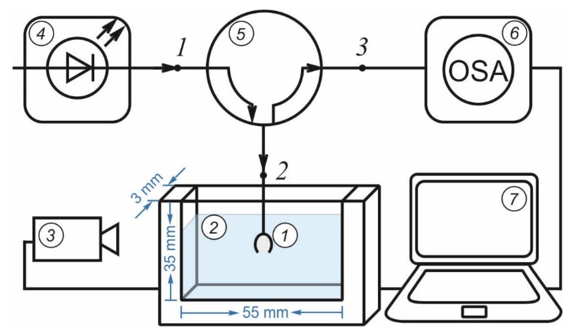
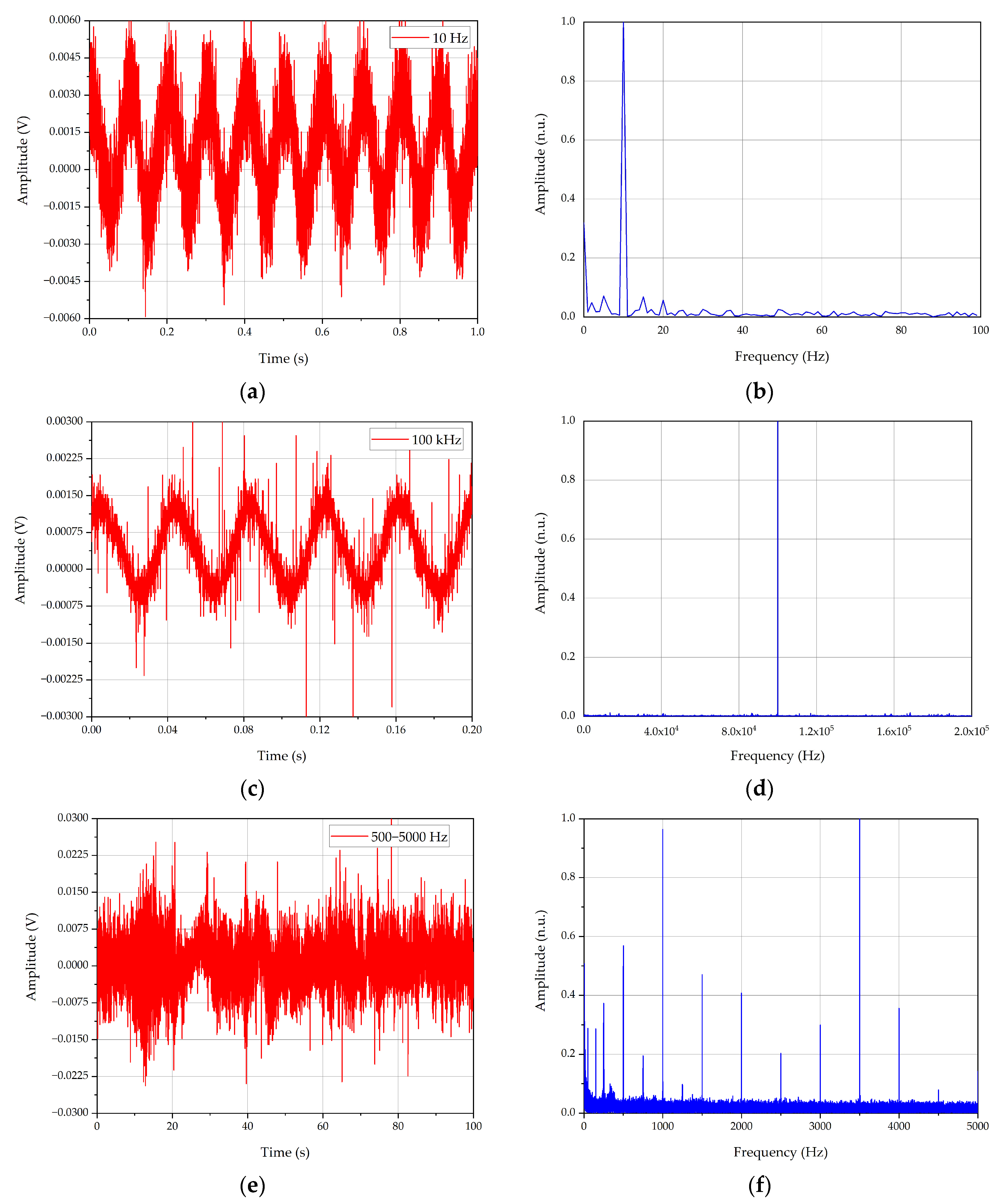
4. Detection of Acoustic Waves in a Liquid

The high sensitivity of the obtained FPI on an open macro-cavity immersed in liquid allows us to use it for the detection of acoustic waves. To test the sensor, an experimental setup was assembled, the scheme of which is shown in Figure 12.

Laser radiation from the tunable narrowband Golight Tunable Light Laser Source—1—(wavelength 1525–1570 nm, half-width 0.16 nm) through port 1 and 2 of the circulator—2—was directed into the optical fiber with the investigated macro-cavity—3. The experiments were carried out at a wavelength of 1550 nm with a radiation power of up to 10 dBm. The fiber end was immersed in the cuvette measuring 5 × 5 × 5 cm—4—filled with water. A speaker—5—was installed at the bottom of the cuvette in the direction of the formed FPI. With the help of the generator GSPF-053, which allows us to vary the shape, frequency, and amplitude of the signal, and the speaker in the water, an acoustic wave was formed, affecting the goodness of the resonator inside the cavity. Using an Avesta OD-007BFC photodetector—6—the time-varying and amplitude-varying signal from the FPI through the circulator (port 3) was recorded on an oscilloscope—7. The signal from the oscilloscope was processed using fast Fourier transform on a PC—8—and converted into a sound file (Supplementary Materials).

Figure 13 shows graphs of the signal amplitude versus time and the frequency spectrum (FFT), normalized to the maximum amplitude, obtained with the input signal of different frequencies: 10 Hz (a,b), 100 kHz (c,d), and frequency varying from 500 Hz to 5 kHz in 500 Hz steps every 10 s (e,f).

To assess the reproducibility of the results, measurements (n = 10) of the selected frequency (500 Hz) were carried out at fixed input parameters of laser radiation (5 dVm) for one of the sensors under study (maximum cavity diameter d = 109.4 µm, opening diameter d′ = 62.5 µm). Experiments showed that, regardless of the amplitude of the detected signal, the accuracy of determining the input frequency was no less than 0.005% and amounted to 500.095 ± 0.028 Hz.

The experiments have shown that the investigated FPI is capable of capturing a signal with frequency in the range from 1 Hz to 100 kHz. The main factors enabling the wide range of detected frequencies are the geometry of the cavity and its opening, and the properties of the ambient liquid (water).

5. Discussion

Based on the results of the study, the technology of creating closed macro-sized cavities inside the optical fiber and open drop-shaped cavities at the end of the optical fiber was developed. We have provided some ways to control the size and shape of such cavities during manufacturing.

A sensor for acoustic oscillations in liquid is proposed on the basis of an open cavity at the end of optical fiber. A mathematical model of the sensor is constructed. Based on the mathematical model, the sensitivity limits of the sensor are investigated. A physical full-scale model of the sensing element is constructed. The dynamic range of measurements is experimentally evaluated.

Primary practical experiments allow us to draw a number of important conclusions:

• The experiment satisfactorily verifies the mathematical model.
• The effect of sensitivity to acoustic vibrations in a liquid of a proposed Fabry-Perot cavity is shown.
• It was initially demonstrated that sensitivity in a certain frequency range is qualitatively observed tens of times from launch to launch of the system, which determines further research paths. The study observed the sensor’s response to frequencies up to 100 kHz, with high repeatability.

Using open drop-shaped cavities, it is possible to create various fiber-optic sensors designed to measure various physical fields, such as temperature, pressure, vibration, strain, current, and so on. The basis of the measurements is the change in the optical signal passing through the sensor, from which a conclusion is made about the magnitude of the physical impact and the value of the measured parameter. Such sensors have common advantages for all fiber optic sensors, such as minimal influence of electromagnetic interference, the possibility of long-term operation in extreme conditions, and a small size.

The open drop-shaped cavity at the end of the fiber can be a versatile element that allows the proposed design to evolve. For example, by placing a transparent and temperature-sensitive material in the cavity, a temperature sensor can be obtained. By closing the open cavity with a membrane, both a pressure sensor and a vibration sensor can be obtained. By placing liquid crystals or ferrofluid in the open cavity and closing the cavity with a non-deformable membrane, it is possible to obtain an electric and magnetic field sensor, since a change in the electric field changes the optical transparency of liquid crystals.

It is also necessary to consider that, under the action of gas diffusion into the liquid phase and capillary effects depending on the surface tension, fluidity, and viscosity, the liquid can flow inside the cavity over time. During the flow, the size of the gas bubble will decrease with time, and at full flow, the interference pattern disappears due to the fact that the second Fabry–Perot mirror disappears. Passing optical radiation through the fiber can cause heating of the gas inside the cavity, which will accelerate the process of the diffusion of the gas bubble into the liquid medium, or will lead to the growth of the bubble which will push the gas phase out of the cavity. The described effects will affect the sensitivity and operation time of the measuring element. And their influence on the sensor operation requires a separate experimental study. Today, there are liquid viscosity and surface tension sensors based on open cavities [44,45,46] which are based on partially filling the cavity with liquid. Our task is to eliminate this effect as much as possible. At the moment, the issue of changing the resonator (the size of the air cavity) over time is being addressed by reducing the wettability of the internal walls of the macro-cavity by applying water-repellent films.

Since this study demonstrates only the initial results of testing an acoustic sensor with high potential, we consider it necessary to state a list of directions of further research. Firstly, careful work is needed to stabilize the sensor parameters, which includes: improving the interferometer manufacturing technology (for example, controlling fuse effect parameters, using special optical fibers, monitoring cavity parameters using optical reflectometry in the frequency domain, stabilization of the parameters of the receiving and transmitting parts of the system, digital signal processing, design of a sensitive membrane. It may be reasonable to start with algorithmic methods, since in our practice we have already encountered a significant improvement in the parameters of acoustic sensors due to signal processing [47]. Secondly, after stabilizing the sensor parameters, it is necessary to evaluate the range of its possible applications. The use of an interferometer of this type in coherent phase-sensitive quasi-distributed fiber-optic sensors has already been started by individual scientific groups. The use of sensors of this kind in fiber-optic flaw detection may be truly relevant.

In the course of this work, a technology for creating a universal element, which is the main technological component of fiber-optic sensors of both open and closed type, based on the Fabry–Perot resonator, has been developed. The high sensitivity of interferometric sensors of this class and their biological compatibility allows us to use them for measurements in living and biologically active tissues. Further research will be dedicated to the usage of the presented developments of the fiber cavities as part of combined fiber-optic sensors with addressed fiber Bragg structures, with the possibility of implementing microwave-photonic interrogation, which will allow to increase the interrogation frequency to dozens or hundreds of gigahertz.

References

1. Fabry, C.; Pérot, A. Sur Les Franges Des Lames Minces Argentées et Leur Application à La Mesure de Petites Épaisseurs d’air. Ann. Chim. Phys. 1897, 12, 459–501. [Google Scholar]
2. Gong, Y.-J.R.; Zeng-Ling, R. Yuan Fiber-Optic Fabry-Perot Sensors: An Introduction; CRC Press: Boca Raton, FL, USA, 2017; ISBN 978-1-315-12099-7. [Google Scholar]
3. Islam, M.R.; Ali, M.; Lai, M.-H.; Lim, K.-S.; Ahmad, H. Chronology of Fabry-Perot Interferometer Fiber-Optic Sensors and Their Applications: A Review. Sensors 2014, 14, 7451–7488. [Google Scholar] [CrossRef] [PubMed]
4. Totsu, K.; Haga, Y.; Esashi, M. Ultra-Miniature Fiber-Optic Pressure Sensor Using White Light Interferometry. J. Micromech. Microeng. 2004, 15, 71. [Google Scholar] [CrossRef]
5. Wang, W.; Wu, N.; Tian, Y.; Niezrecki, C.; Wang, X. Miniature All-Silica Optical Fiber Pressure Sensor with an Ultrathin Uniform Diaphragm. Opt. Express 2010, 18, 9006–9014. [Google Scholar] [CrossRef]
6. Duraibabu, D.B.; Poeggel, S.; Omerdic, E.; Capocci, R.; Lewis, E.; Newe, T.; Leen, G.; Toal, D.; Dooly, G. An Optical Fibre Depth (Pressure) Sensor for Remote Operated Vehicles in Underwater Applications. Sensors 2017, 17, 406. [Google Scholar] [CrossRef] [PubMed]
7. Wang, W.; Li, F. Large-Range Liquid Level Sensor Based on an Optical Fibre Extrinsic Fabry–Perot Interferometer. Opt. Lasers Eng. 2014, 52, 201–205. [Google Scholar] [CrossRef]
8. Liu, S.; Wang, Y.; Liao, C.; Wang, Y.; He, J.; Fu, C.; Yang, K.; Bai, Z.; Zhang, F. Nano Silica Diaphragm In-Fiber Cavity for Gas Pressure Measurement. Sci. Rep. 2017, 7, 787. [Google Scholar] [CrossRef]
9. Cibula, E.; Ðonlagić, D. Miniature Fiber-Optic Pressure Sensor with a Polymer Diaphragm. Appl. Opt. 2005, 44, 2736–2744. [Google Scholar] [CrossRef]
10. Xu, F.; Ren, D.; Shi, X.; Li, C.; Lu, W.; Lu, L.; Lu, L.; Yu, B. High-Sensitivity Fabry–Perot Interferometric Pressure Sensor Based on a Nanothick Silver Diaphragm. Opt. Lett. 2012, 37, 133–135. [Google Scholar] [CrossRef]
11. Ma, J.; Jin, W.; Ho, H.L.; Dai, J.Y. High-Sensitivity Fiber-Tip Pressure Sensor with Graphene Diaphragm. Opt. Lett. 2012, 37, 2493–2495. [Google Scholar] [CrossRef]
12. Cheng, L.; Wang, C.; Huang, Y.; Liang, H.; Guan, B.-O. Silk Fibroin Diaphragm-Based Fiber-Tip Fabry-Perot Pressure Sensor. Opt. Express 2016, 24, 19600–19606. [Google Scholar] [CrossRef] [PubMed]
13. Luo, C.; Liu, X.; Liu, J.; Shen, J.; Li, H.; Zhang, S.; Hu, J.; Zhang, Q.; Wang, G.; Huang, M. An Optimized PDMS Thin Film Immersed Fabry-Perot Fiber Optic Pressure Sensor for Sensitivity Enhancement. Coatings 2019, 9, 290. [Google Scholar] [CrossRef]
14. Wei, X.; Song, X.; Li, C.; Hou, L.; Li, Z.; Li, Y.; Ran, L. Optical Fiber Gas Pressure Sensor Based on Polydimethylsiloxane Microcavity. J. Light. Technol. 2021, 39, 2988–2993. [Google Scholar] [CrossRef]
15. Cheng, X.; Dash, J.N.; Gunawardena, D.S.; Htein, L.; Tam, H.-Y. Silicone Rubber Based Highly Sensitive Fiber-Optic Fabry–Perot Interferometric Gas Pressure Sensor. Sensors 2020, 20, 4927. [Google Scholar] [CrossRef] [PubMed]
16. Zhang, Y.; Zhang, S.; Gao, H.; Xu, D.; Gao, Z.; Hou, Z.; Shen, J.; Li, C. A High Precision Fiber Optic Fabry–Perot Pressure Sensor Based on AB Epoxy Adhesive Film. Photonics 2021, 8, 581. [Google Scholar] [CrossRef]
17. Zhu, C.; Chen, Y.; Zhuang, Y.; Fang, G.; Liu, X.; Huang, J. Optical Interferometric Pressure Sensor Based on a Buckled Beam With Low-Temperature Cross-Sensitivity. IEEE Trans. Instrum. Meas. 2018, 67, 950–955. [Google Scholar] [CrossRef]
18. Li, J.; Jia, P.; Fang, G.; Wang, J.; Qian, J.; Ren, Q.; Xiong, J. Batch-Producible All-Silica Fiber-Optic Fabry–Perot Pressure Sensor for High-Temperature Applications up to 800 °C. Sens. Actuators A Phys. 2022, 334, 113363. [Google Scholar] [CrossRef]
19. Wu, J.; Yao, M.; Xiong, F.; Zhang, A.P.; Tam, H.-Y.; Wai, P.K.A. Optical Fiber-Tip Fabry–Pérot Interferometric Pressure Sensor Based on an In Situ μ-Printed Air Cavity. J. Light. Technol. 2018, 36, 3618–3623. [Google Scholar] [CrossRef]
20. Cui, Q.; Thakur, P.; Rablau, C.; Avrutsky, I.; Cheng, M.M.-C. Miniature Optical Fiber Pressure Sensor With Exfoliated Graphene Diaphragm. IEEE Sens. J. 2019, 19, 5621–5631. [Google Scholar] [CrossRef]
21. Domingues, M.F.; Paixão, T.; Mesquita, E.; Alberto, N.; Antunes, P.; Varum, H.; André, P.S. Hydrostatic Pressure Sensor Based on Micro-Cavities Developed by the Catastrophic Fuse Effect. In Proceedings of the 24th International Conference on Optical Fibre Sensors, Curitiba, Brazil, 28 September 2015; SPIE: Bellingham, WA, USA, 2015; Volume 9634, pp. 737–740. [Google Scholar]
22. Martins, J.; Diaz, C.A.R.; Domingues, M.F.; Ferreira, R.A.S.; Antunes, P.; André, P.S. Low-Cost and High-Performance Optical Fiber-Based Sensor for Liquid Level Monitoring. IEEE Sens. J. 2019, 19, 4882–4888. [Google Scholar] [CrossRef]
23. Ferreira, L.A.; Lobo Ribeiro, A.B.; Santos, J.L.; Farahi, F. Simultaneous Measurement of Displacement and Temperature Using a Low Finesse Cavity and a Fiber Bragg Grating. IEEE Photonics Technol. Lett. 1996, 8, 1519–1521. [Google Scholar] [CrossRef]
24. Bremer, K.; Lewis, E.; Leen, G.; Moss, B.; Lochmann, S.; Mueller, I.A.R. Feedback Stabilized Interrogation Technique for EFPI/FBG Hybrid Fiber-Optic Pressure and Temperature Sensors. IEEE Sens. J. 2012, 12, 133–138. [Google Scholar] [CrossRef]
25. Poeggel, S.; Duraibabu, D.; Kalli, K.; Leen, G.; Dooly, G.; Lewis, E.; Kelly, J.; Munroe, M. Recent Improvement of Medical Optical Fibre Pressure and Temperature Sensors. Biosensors 2015, 5, 432–449. [Google Scholar] [CrossRef] [PubMed]
26. Wang, Q.; Yu, Q. Polymer Diaphragm Based Sensitive Fiber Optic Fabry-Perot Acoustic Sensor. Chin. Opt. Lett. COL 2010, 8, 266–269. [Google Scholar] [CrossRef]
27. Gong, Z.; Chen, K.; Zhou, X.; Yang, Y.; Zhao, Z.; Zou, H.; Yu, Q. High-Sensitivity Fabry-Perot Interferometric Acoustic Sensor for Low-Frequency Acoustic Pressure Detections. J. Light. Technol. 2017, 35, 5276–5279. [Google Scholar] [CrossRef]
28. Xu, F.; Shi, J.; Gong, K.; Li, H.; Hui, R.; Yu, B. Fiber-Optic Acoustic Pressure Sensor Based on Large-Area Nanolayer Silver Diaghragm. Opt. Lett. 2014, 39, 2838–2840. [Google Scholar] [CrossRef] [PubMed]
29. Fan, P.; Yan, W.; Lu, P.; Zhang, W.; Zhang, W.; Fu, X.; Zhang, J. High Sensitivity Fiber-Optic Michelson Interferometric Low-Frequency Acoustic Sensor Based on a Gold Diaphragm. Opt. Express 2020, 28, 25238–25249. [Google Scholar] [CrossRef]
30. Wang, S.; Lu, P.; Liu, L.; Liao, H.; Sun, Y.; Ni, W.; Fu, X.; Jiang, X.; Liu, D.; Zhang, J.; et al. An Infrasound Sensor Based on Extrinsic Fiber-Optic Fabry–Perot Interferometer Structure. IEEE Photonics Technol. Lett. 2016, 28, 1264–1267. [Google Scholar] [CrossRef]
31. Liu, B.; Zheng, G.; Wang, A.; Gui, C.; Yu, H.; Shan, M.; Jin, P.; Zhong, Z. Optical Fiber Fabry–Perot Acoustic Sensors Based on Corrugated Silver Diaphragms. IEEE Trans. Instrum. Meas. 2020, 69, 3874–3881. [Google Scholar] [CrossRef]
32. Ma, J.; Xuan, H.; Ho, H.L.; Jin, W.; Yang, Y.; Fan, S. Fiber-Optic Fabry–Pérot Acoustic Sensor With Multilayer Graphene Diaphragm. IEEE Photonics Technol. Lett. 2013, 25, 932–935. [Google Scholar] [CrossRef]
33. Ni, W.; Lu, P.; Fu, X.; Zhang, W.; Shum, P.P.; Sun, H.; Yang, C.; Liu, D.; Zhang, J. Ultrathin Graphene Diaphragm-Based Extrinsic Fabry-Perot Interferometer for Ultra-Wideband Fiber Optic Acoustic Sensing. Opt. Express 2018, 26, 20758–20767. [Google Scholar] [CrossRef] [PubMed]
34. Guo, M.; Chen, K.; Yang, B.; Li, C.; Zhang, B.; Yang, Y.; Wang, Y.; Li, C.; Gong, Z.; Ma, F.; et al. Ultrahigh Sensitivity Fiber-Optic Fabry–Perot Interferometric Acoustic Sensor Based on Silicon Cantilever. IEEE Trans. Instrum. Meas. 2021, 70, 1–8. [Google Scholar] [CrossRef]
35. De Fatima, F.; Domingues, M.; De Brito Paixao, T.; Mesquita, E.F.T.; Alberto, N.; Frias, A.R.; Ferreira, R.A.S.; Varum, H.; Da Costa Antunes, P.F. Liquid Hydrostatic Pressure Optical Sensor Based on Micro-Cavity Produced by the Catastrophic Fuse Effect. IEEE Sens. J. 2015, 15, 5654–5658. [Google Scholar] [CrossRef]
36. Xiao, Q.; Tian, J.; Yan, P.; Li, D.; Gong, M. Exploring the Initiation of Fiber Fuse. Sci. Rep. 2019, 9, 11655. [Google Scholar] [CrossRef] [PubMed]
37. Rocha, A.M.; Da Costa Antunes, P.F.; De Fatima, F.; Domingues, M.; Facao, M.; De Brito Andre, P.S. Detection of Fiber Fuse Effect Using FBG Sensors. IEEE Sens. J. 2011, 11, 1390–1394. [Google Scholar] [CrossRef]
38. Antunes, P.F.C.; Domingues, M.F.F.; Alberto, N.J.; Andre, P.S. Optical Fiber Microcavity Strain Sensors Produced by the Catastrophic Fuse Effect. IEEE Photonics Technol. Lett. 2014, 26, 78–81. [Google Scholar] [CrossRef]
39. Domingues, F.; Frias, A.R.; Antunes, P.; Sousa, A.O.P.; Ferreira, R.A.S.; André, P.S. Observation of Fuse Effect Discharge Zone Nonlinear Velocity Regime in Erbium-Doped Fibres. Electron. Lett. 2012, 48, 1295. [Google Scholar] [CrossRef]
40. Konin, Y.A.; Scherbakova, V.A.; Bulatov, M.I.; Malkov, N.A.; Lucenko, A.S.; Starikov, S.S.; Grachev, N.A.; Perminov, A.V.; Petrov, A.A. Structural Characteristics of Internal Microcavities Produced in Optical Fiber via the Fuse Effect. J. Opt. Technol. 2021, 88, 672. [Google Scholar] [CrossRef]
41. Kashyap, R. The Fiber Fuse—From a Curious Effect to a Critical Issue: A 25^th Year Retrospective. Opt. Express 2013, 21, 6422. [Google Scholar] [CrossRef]
42. Kutsche, I.; Gildehaus, G.; Schuller, D.; Schumpe, A. Oxygen Solubilities in Aqueous Alcohol Solutions. J. Chem. Eng. Data 1984, 29, 286–287. [Google Scholar] [CrossRef]
43. Agliullin, T.; Anfinogentov, V.; Morozov, O.; Sakhabutdinov, A.; Valeev, B.; Niyazgulyeva, A.; Garovov, Y. Comparative Analysis of the Methods for Fiber Bragg Structures Spectrum Modeling. Algorithms 2023, 16, 101. [Google Scholar] [CrossRef]
44. Zhu, Y.; Kang, J.; Sang, T.; Dong, X.; Zhao, C. Hollow Fiber-Based Fabry–Perot Cavity for Liquid Surface Tension Measurement. Appl. Opt. 2014, 53, 7814–7818. [Google Scholar] [CrossRef] [PubMed]
45. Tian, Y.; Xu, B.; Chen, Y.; Duan, C.; Tan, T.; Chai, Q.; Carvajal Martí, J.J.; Zhang, J.; Yang, J.; Yuan, L. Liquid Surface Tension and Refractive Index Sensor Based on a Side-Hole Fiber Bragg Grating. IEEE Photonics Technol. Lett. 2019, 31, 947–950. [Google Scholar] [CrossRef]
46. Tian, Y.; Xiao, G.; Luo, Y.; Zhang, J.; Yuan, L. Microhole Fiber-Optic Sensors for Nanoliter Liquid Measurement. Opt. Fiber Technol. 2022, 72, 102981. [Google Scholar] [CrossRef]
47. Turov, A.T.; Barkov, F.L.; Konstantinov, Y.A.; Korobko, D.A.; Lopez-Mercado, C.A.; Fotiadi, A.A. Activation Function Dynamic Averaging as a Technique for Nonlinear 2D Data Denoising in Distributed Acoustic Sensors. Algorithms 2023, 16, 440. [Google Scholar] [CrossRef]
Figure 1. Photo of the optical fiber (a) with a core containing micro-cavities formed by plasma melting; (b) structure of the inner surface of the micro-cavity.
Photonics 11 00022 g001
Figure 2. The dependence of the cavity size and shape on the discharge arc power: (a) P = 0%, d = 79.8 μm; (b) P = 10%, d = 79.8 μm; (c) P = 20%, d = 91.2 μm; (d) P = 30%, d = 125.4 μm; (e) P = 50%, d = 125.4 μm; (f) P = 70%, d = 125.4 μm; discharge arc duration 2 s.
Photonics 11 00022 g002
Figure 3. The cavity size and shape depending on the discharge arc duration: (a) t = 500 ms, d = 57 µm; (b) t = 1000 ms, d = 102.6 µm; (c) t = 1500 ms, d = 102.5 µm; (d) t = 2000 ms, d = 91.2 µm; (e) t = 2500 ms, d = 102.6 µm; (f) t = 3000 ms, d = 114 µm; (g) t = 3500 ms, d = 91.2 µm; (h) t = 4000 ms, d = 91.2 µm. The arc discharge power was 20%.
Photonics 11 00022 g003
Figure 4. (a) Photograph of a drop-shaped cavity on the end of an optical fiber immersed in water; (b) reflection spectrum (black—fiber end in air; red—fiber end immersed in isopropanol; blue—fiber end immersed in water).
Photonics 11 00022 g004
Figure 5. Diagram of the experimental setup: 1—sensitive element; 2—Hele-Shaw cell; 3—digital camera; 4—broadband laser; 5—optical circulator; 6—optical spectrum analyzer; 7—PC.
Photonics 11 00022 g005
Figure 6. Axisymmetric cavity at the end of an optical fiber: (a) microphotograph; (b) schematic of the cavity immersed in liquid.
Photonics 11 00022 g006
Figure 7. The simplest model of light radiation propagation through an air-filled cavity lowered into a liquid.
Photonics 11 00022 g007
Figure 8. Reflection coefficient in the wavelength range from λMin = 1510 to λMax = 1590 nm.
Photonics 11 00022 g008
Figure 9. Reflection coefficient at λL = 1553.36 nm, L = 1.0 × 10⁻⁴ m, and ΔL = 0.3 × 10⁻⁶ m.
Photonics 11 00022 g009
Figure 10. Reflection coefficient at λL = 1553.36 nm, L = 1.0 × 10⁻⁴ m, and ΔL = 1.0 × 10⁻⁷ m.
Photonics 11 00022 g010
Figure 11. Reflection coefficient at λL = 1553.36 nm, L = 1.0 × 10⁻⁴ m, and ΔL = 1.0 nm.
Photonics 11 00022 g011
Figure 12. Scheme of the experimental setup: 1—tunable narrow-band laser; 2—optical circulator; 3—macro-cavity; 4—cuvette with water; 5—speaker; 6—photodetector; 7—oscilloscope; 8—PC.
Photonics 11 00022 g012
Figure 13. Oscillograms and spectra (FFT), obtained with the input signal of different frequencies: 10 Hz (a,b), 100 kHz (c,d), frequency varying from 500 Hz to 5 kHz in 500 Hz steps every 10 s (e,f).
Photonics 11 00022 g013
Disclaimer/Publisher’s Note: The statements, opinions and data contained in all publications are solely those of the individual author(s) and contributor(s) and not of MDPI and/or the editor(s). MDPI and/or the editor(s) disclaim responsibility for any injury to people or property resulting from any ideas, methods, instructions or products referred to in the content.