A Comprehensive Study on Phase Sensitive Amplification and Stimulated Brillouin Scattering in Nonlinear Fibers with Longitudinally Varying Dispersion

Abstract

Fiber optic parametric and phase sensitive amplifiers (PSA) are interesting for modern day communication technologies due to their low noise and high gain amplification properties with a potential for all optical signal processing and wide band operation. PSAs are typically employed in either a single pump or dual pump configuration. In this article we explore the utilities of both configurations, however considering a fiber with a longitudinally varying dispersion profile. For the single pump case, PSA operation at large pump-signal detunings, that arise due to the longitudinal dispersion variation, were studied numerically, and recipes of using the system as a wide band wavelength selective filter were laid out. For the dual-pump case, emphasis was laid on achieving a larger signal gain, by reducing stimulated Brillouin scattering (SBS) that prevents large pump power transport through the nonlinear fiber. First, the effects of dispersion variation on the gain of a dual pump PSA were studied analytically and numerically in order to optimize the dispersion variation profile, neglecting SBS processes. Then we independently studied the SBS dynamics of the system numerically. A sinusoidally dispersion oscillating fiber (DOF) was found to be an optimal candidate with respect to its PSA and SBS performances. To establish this claim, we also experimentally compared the performance of an available DOF over a standard highly nonlinear fiber (HNLF) that has a constant dispersion profile and established its utility for designing a high gain PSA system, thanks to the SBS mitigation due to the longitudinal dispersion variation of the fiber.

1. Introduction

Fiber-optic parametric amplifiers (FOPA) in a phase sensitive amplification (PSA) configuration are capable of providing noiseless (ideally 0 dB noise figure) optical amplification, while other phase insensitive amplifiers like Erbium Doped Fiber Amplifiers (EDFA) are always limited by a noise figure of at least 3 dB [1,2,3,4]. This attribute of noiseless amplification of PSAs have attracted recent attention in terms of their potential applications in a variety of domains such as microwave photonics, all optical signal processing, long-haul optical communication, free-space satellite communication, quantum technologies, etc. to name a few [5,6,7,8,9,10]. Recent progresses in the field have led to exploration of unconventional fiber designs in terms of the longitudinal variation of the fiber dispersion along the fiber length for system performance enhancements in diverse fiber-optic application platforms [11,12,13,14]. In this article, we aim to provide a comprehensive investigation of the utility of employing a nonlinear fiber with longitudinally varying dispersion, aimed at developing a high-performance PSA system with different pump configurations.

PSAs demand the use of a highly nonlinear medium. In

Table 1. Table for comparison of advantages and disadvantages of different nonlinear media.

Nonlinear Medium	Advantage	Disadvantage
Highly nonlinear fiber (HNLF)	High gain and low noise figure; Typical nonlinear coefficient is high, ∼10 (W  km)−1	High power required to invoke nonlinearities, low stimulated Brillouin scattering (SBS) threshold
Periodically poled Lithium Niobate (PPLN)	Moderate gain and compact	High power required to invoke nonlinearities
Semiconductor optical amplifier (SOA)	Compact	High noise figure
Dispersion oscillating fiber (DOF)	High SBS threshold, low noise figure, moderate (potentially large) gain	High power required to invoke nonlinearities since experimental nonlinear coefficient in this work is 3.5 (W km)−1. However this value can be increased by using a preform of a HNLF

we provide a short list of different commonly used nonlinear media employed in various applications. When compared to other nonlinear media, DOFs, that are fibers with an oscillating longitudinal dispersion profile, are potential candidates for accessing a larger nonlinearity in the system [15]. This is possible because of large pump powers could be launched into DOFs owing to a potentially lower stimulated Brillouin scattering (SBS) compared to a conventional HNLF, as we will discuss later in detail.

Typically PSAs are operated in a single or dual pump configuration. While single pump configurations are often preferred for low distortion signal amplification [16], or in general, in scenarios where the signal gain is not a key performance metric, a dual pump configuration is preferred in applications requiring a large PSA signal gain, ideally with polarisation insensitive operation. Single pump optical parametric amplification with fibers having a longitudinally oscillating dispersion profile, or in other words dispersion oscillating fibers (DOF) were initially investigated in the context of dispersion management in long-haul optical communication links [17]. These investigations, that predicted the presence of high-order modulation instability sidebands in a DOF gain spectrum made it an interesting candidate for other applications such as frequency conversion [13] and wide band optical parametric amplification [18]. However, the use of DOFs as a single pump PSA is still an open area of research to the best of our knowledge. Furthermore, with the continual development of newer all optical signal processing capabilities of PSA based systems [19,20,21,22], albeit using multiple pumps, we plan to investigate a single pump DOF based PSA system, where the dispersion variation provides us with an extra degree of freedom for tailoring the system functionalities. To this aim we investigate analytically and numerically the physics of the signal amplification in a DOF acting as a single pump PSA and unravel the relationship between the dispersion profile with various system parameters and investigate its potential for developing wavelength selective wide band tunable filters for optical signal processing applications.

Contrary to the single pump configuration, the dual pump configuration enjoys the advantage of not requiring a copier stage for achieving PSA functionality when operated in a degenerate signal-idler mode [5,23]. Recently, the case of a dual-pump PSA with a dispersion oscillating fiber was investigated analytically in [24]. However, the question of whether a sinusoidal dispersion profile is the optimal profile for attaining a large PSA gain is still an open one. Therefore, in this article we also address the question, what is the optimal non-constant dispersion profile for achieving a large PSA gain for practical applications?

Although FOPA-based dual pump PSAs provide an exquisite combination of low noise and high gain modality, achieving a high gain in practice is often challenging due to energy loss from stimulated Brillouin scattering (SBS) within the fiber. SBS prevents transmission of high power, highly coherent pump waves through long lengths of nonlinear fiber due to the coherent build up of Stokes wave in the counter-propagating direction. In order to get around the power scaling inhibition posed by SBS within a nonlinear fiber, several approaches had been adopted, such as applying a distributed strain [25,26], applying a temperature gradient along the fiber length [27,28], broadening the pump linewidth through phase modulation [29,30,31,32,33], etc. to name a few. Introduction of air gaps and tapers were also attempted for SBS mitigation with scanty success nonetheless [34]. While application of temperature and strain gradients are prone to fluctuations and are cumbersome in terms of commercial deployments, phase modulation techniques pose a different challenge in PSA systems. In a PSA, the signal gain is sensitive to the relative phase difference between the two pumps and the degenerate signal (considering a dual-pump configuration) [35]. Therefore, phase modulation of the pumps induce different phases for the different modulation tones and hence degrades the PSA gain extinction ratio of the system [36]. For a dual pump configuration, synchronous phase modulation of the pumps can avoid such effects [37], however such active processes come with additional complexity and often is detrimental for the noise performance of the system. Another remedy towards the SBS problem runs in the lines of varying the properties of the fiber along the fiber length, dispersion being one of them [15,24,38]. Dispersion variation along the fiber length can be achieved by varying the radius of the fiber preform along the length while pulling it from a drawing tower. Here we consider a W-type refractive index of the preform as shown in Figure 1 as is standard for commercial highly nonlinear fibers (HNLF). Since the waveguide dispersion is a function of the core radius, the variation of the dispersion along the fiber length can potentially inhibit the build-up of the different acoustic modes that interact with the optical pump modes that generate the SBS process. Therefore another dimension of our investigation focuses on analyzing the SBS dynamics in a DOF using a steady-state numerical approach. We further investigate multiple longitudinally varying radius profiles and propose optimal designs for SBS mitigation, that in turn complements our goal of designing a high-gain dual pump PSA system. Furthermore, the SBS advantage of a DOF over a conventional highly nonlinear fiber (HNLF) was experimentally confirmed with an available DOF. We also numerically and experimentally compared the four wave mixing (FWM) conversion efficiency (CE), which is a key quantifier for any PSA system, of the available DOF and HNLF.

This paper is organized as follows. In Section 2, we focus on the numerical calculation of the dispersion properties of the fiber. Section 3 and Section 4 deal with investigating the PSA performance of dispersion tailored fibers, in single and dual pump configurations respectively. In Section 5 we numerically investigate the SBS threshold of DOFs and identify optimized profiles for further elevating the SBS threshold. Then in Section 6 we provide experimental results on SBS mitigation in a DOF and quantify the conversion efficiency (CE) of a DOF as a parametric amplifier. Henceforth in Section 7 we discuss the implications of the obtained numerical and experimental results. Finally in Section 8 we summarize the findings and conclude the key takeaways of this paper.

2. Fiber Parameters

Modification in the SBS and PSA properties are proposed in this paper by changing the material and geometric properties of the optical fiber along the radius and length. Hence, before proceeding further with the investigation on SBS and PSA, first we need to calculate the dispersion and nonlinear characteristics of the fiber, with respect to its material and geometric properties, which are described in this section.

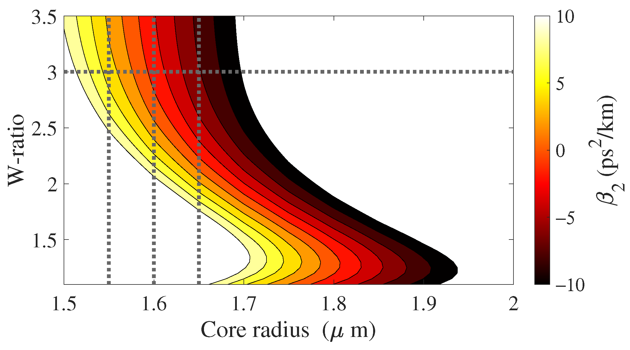
2.1. Dispersion Parameters

The total dispersion, i.e., chromatic dispersion in any waveguide arises from the combined effect of material dispersion and waveguide dispersion. Material dispersion is a result of the dependence of refractive index on the wavelength of light in that particular material. On the other hand, waveguide dispersion arise from the spectral dependence of the propagation constants of the modes supported by the waveguide. Since the modal properties depend on the geometry of the waveguide, the total dispersion of the propagating modes heavily depend on the fiber geometry in the case of optical fibers.

In this work, we consider a W-type fiber design, that consists of a narrow core of larger refractive index (RI) at the center, followed by an annular trench of low RI and another annular cladding of intermediate RI at the periphery (see Figure 1). The refractive index $RI$ profile of the W-type fiber is defined as a function of the radial distance r (transversal to the fiber) as:

$$RI\left(r\right)=\left\{\begin{array}{cc}{N}_1\hfill & 0\le r<\frac{a}{2}\hfill \\ N_2\hfill & \frac{a}{2}\le r<\frac{b}{2}\hfill \\ N_3\hfill & r\ge \frac{b}{2}\hfill \end{array}\right.$$

(1)

For our geometry, $N_1>N_3>N_2$. We consider a weakly guiding case, i.e., $N_1-N_2$ and $N_2-N_3$ are small. The mode field $\psi (r,\varphi )$, where $\varphi$ is the azimuthal angle in the cylindrical coordinate system is governed by [23]:

$$\frac{{\partial }^2\psi }{\partial r^2}+\frac{1}{r}\frac{\partial \psi }{\partial r}+\frac{1}{r^2}\frac{{\partial }^2\psi }{\partial {\varphi }^2}+(k_0^2{\nu }^2-{\beta }^2)\psi =0,$$

(2)

where $k_0$ is the free space wave number and $\nu$ is the refractive index of silica. We rewrite Equation (2) as an eigenvalue equation as:

$$[{\nabla }_t^2+k_0^2{\nu }^2]\psi ={\beta }^2\psi ,$$

(3)

where ${\nabla }_t$ is the transverse Laplacian operator. Then using a mode solver, we found the eigenvalues, i.e., $\beta$ for different core radii, wavelength and W-ratio. The numerical calculations for evaluation of $\beta$ were validated with the data provided in Ref. [39]. Also, within a core radius of 2.3 $\mathsf{\mu }$m, a single mode operation was ensured.

In order to find the dispersion coefficients, the propagation constant $\beta \left(\omega \right)$, is found as a function of frequency, $\omega$ and is expanded around a central angular frequency ${\omega }_0$ in a Taylor series. As is standard in PSA calculations, truncating the series up to fourth order terms gives us:

$$\beta \left(\omega \right)\approx {\beta }_0+{\beta }_1(\omega -{\omega }_0)+{\beta }_2\frac{{(\omega -{\omega }_0)}^2}{2}+{\beta }_3\frac{{(\omega -{\omega }_0)}^3}{6}+{\beta }_4\frac{{(\omega -{\omega }_0)}^4}{24},$$

(4)

where ${\beta }_m={\left(\frac{d^m\beta }{d{\omega }^m}\right)}_{\omega ={\omega }_0}$ with $m=1, 2, 3, 4$. Throughout our discussion, we will adhere to a maximum value of $m=4$, except for the analytical modeling, where m is often truncated to 2. In Figure 2, we plot ${\beta }_2$ (a), ${\beta }_3$ (b) and ${\beta }_4$ (c) as a function of the core radius and the W-ratio.

For a DOF, the longitudinal variation of the m-th order dispersion ${\beta }_m$ is defined as:

$${\beta }_m\left(z\right)={\overline{\beta }}_m+{\tilde{\beta }}_{m}sin\left(\frac{2\pi z}{z_{\mathrm{mod}}}+{\phi }_{\mathrm{mod}}\right),$$

(5)

where ${\overline{\beta }}_m$ is the average m-th order dispersion, ${\tilde{\beta }}_m$ is the strength of dispersion modulation, $z_{\mathrm{mod}}$ and ${\phi }_{\mathrm{mod}}$ are the wavelength and phase of the modulation respectively. z is the light propagation direction.

2.2. Nonlinear Coefficient

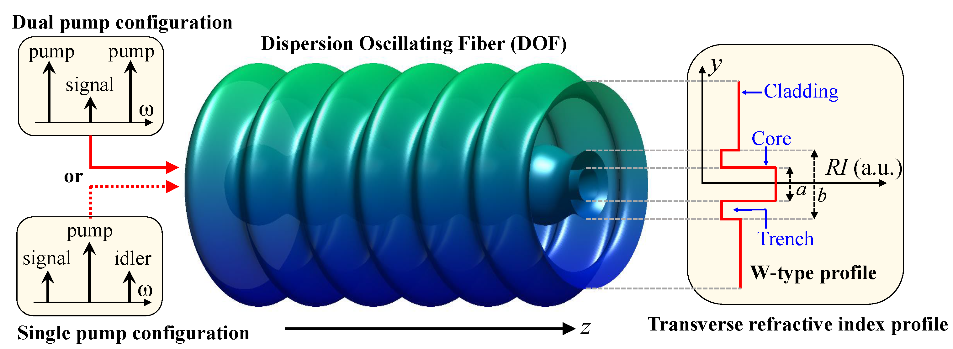
The nonlinear coefficient of a fiber typically depends on the doping concentrations of the core and the cladding. In a DOF, due to the variation of the core radius along the fiber length, the effective mode area changes. This in principle should also change the nonlinear coefficient $\gamma$. In fact, the mode area can be computed from the mode solver straight forwardly. From the standard literature, we know however, that the variation of $\gamma$ in a DOF with ${\tilde{\beta }}_2$ of the order of a few tens of ps²/km is small and can be neglected [14]. The nominal value of nonlinear parameter for this is typically of the order of 5 ${\left(\mathrm{W}\mathrm{km}\right)}^{-1}$.

3. PSA in a DOF

PSA implementations commonly involve two configurations: 1. single pump configuration where a non degenerate signal and idler along with a strong pump are launched at the fiber input (see Figure 3), and 2. dual pump configuration, where the signal (or idler) at the input is degenerate and two non degenerate pumps are launched along with it.

To study the field propagation in the DOF we use local mode approach [40]. The local mode approach requires slow variation of the fiber core. In a single-mode fiber the criterion for slow variation is $z_b\ll z_{\mathrm{mod}}$, where $z_b=2\pi {(\beta -k_0{N}_3)}^{-1}$ is the beat length between the fundamental and cladding mode. Calculation of the beat length gives the value, which does not exceed ${10}^{-3}$ m. In our study, the modulation period $z_{\mathrm{mod}}$ is tens of meters. So the slow variation criterion $z_b\ll z_{\mathrm{mod}}$ is satisfied. We consider the propagation of three stationary copolarized waves with slowly varying complex amplitudes $A_0,A_{-1}$ and $A_1$, which represent the electric fields at the frequencies ${\omega }_0$, ${\omega }_{-1}={\omega }_0-{\Omega }_{ps}$ and ${\omega }_1={\omega }_0+{\Omega }_{ps}$, where ${\Omega }_{ps}$ is the pump-signal angular frequency separation. The total transverse electric field propagating along the single-mode DOF may be written as [35,40]

$$\begin{array}{c}\hfill E(x,y,z,t)=\frac{1}{2}\frac{f(x,y)}{{\left(nc{\epsilon }_0{A}_{\mathrm{eff}}\right)}^{1/2}}\left[A_0\left(z\right)exp\left(i{\int }_0^z\beta ({\omega }_0,z^{\prime })dz-i{\omega }_{0}t\right)\right.\\ \hfill +A_{-1}\left(z\right)exp\left(i{\int }_0^z\beta ({\omega }_{-1},z^{\prime })dz-i{\omega }_{-1}t\right)\\ \hfill \left.+A_1\left(z\right)exp\left(i{\int }_0^z\beta ({\omega }_1,z^{\prime })dz-i{\omega }_{1}t\right)+\mathrm{c}.\mathrm{c}.\right],\end{array}$$

(6)

where $f(x,y)$ is the common transverse modal profile which is assumed to be identical for all three waves along the fiber, n is the effective index of optical mode, c is the speed of light in vacuum, ${\epsilon }_0$ is the vacuum permittivity, $A_{\mathrm{eff}}$ is the effective mode area averaged over the fiber length. As discussed in Section 2.2, we neglect the variation of the transverse mode profile along the fiber length. Due to the denominator ${\left(nc{\epsilon }_0{A}_{\mathrm{eff}}\right)}^{1/2}$ in (6) the values of $|A_0{|}^2$ and $|A_{\pm 1}{|}^2$ are in terms of Watts. Starting from wave equation (see Chapter 2 in [35]), it is straightforward to derive three coupled ordinary differential equations for $A_0,A_{-1}$ and $A_1$ [35,41]

$$\begin{array}{ccc}\hfill \frac{d{A}_0}{dz}& =& i\gamma \left(\right|A_0{|}^2+2|A_{-1}{|}^2+2|A_1{|}^2)A_0+2i\gamma A_0^{*}{A}_{-1}{A}_1{e}^{i\xi \left(z\right)}-\frac{\alpha }{2}{A}_0,\hfill \end{array}$$

(7)

$$\begin{array}{ccc}\hfill \frac{d{A}_{\pm 1}}{dz}& =& i\gamma \left(2\right|A_0{|}^2+2|A_{\mp 1}{|}^2+|A_{\pm 1}{|}^2)A_{\pm 1}+i\gamma A_0^2{A}_{\mp 1}^{*}{e}^{-i\xi \left(z\right)}-\frac{\alpha }{2}{A}_{\pm 1},\hfill \end{array}$$

(8)

where $\alpha$ is the attenuation coefficient. The linear phase mismatch is

$$\xi \left(z\right)={\int }_0^z\beta ({\omega }_{-1},z^{\prime })+\beta ({\omega }_1,z^{\prime })-2\beta ({\omega }_0,z^{\prime })d{z}^{\prime }$$

(9)

3.1. Analytical Model of the PSA: Single Pump Configuration

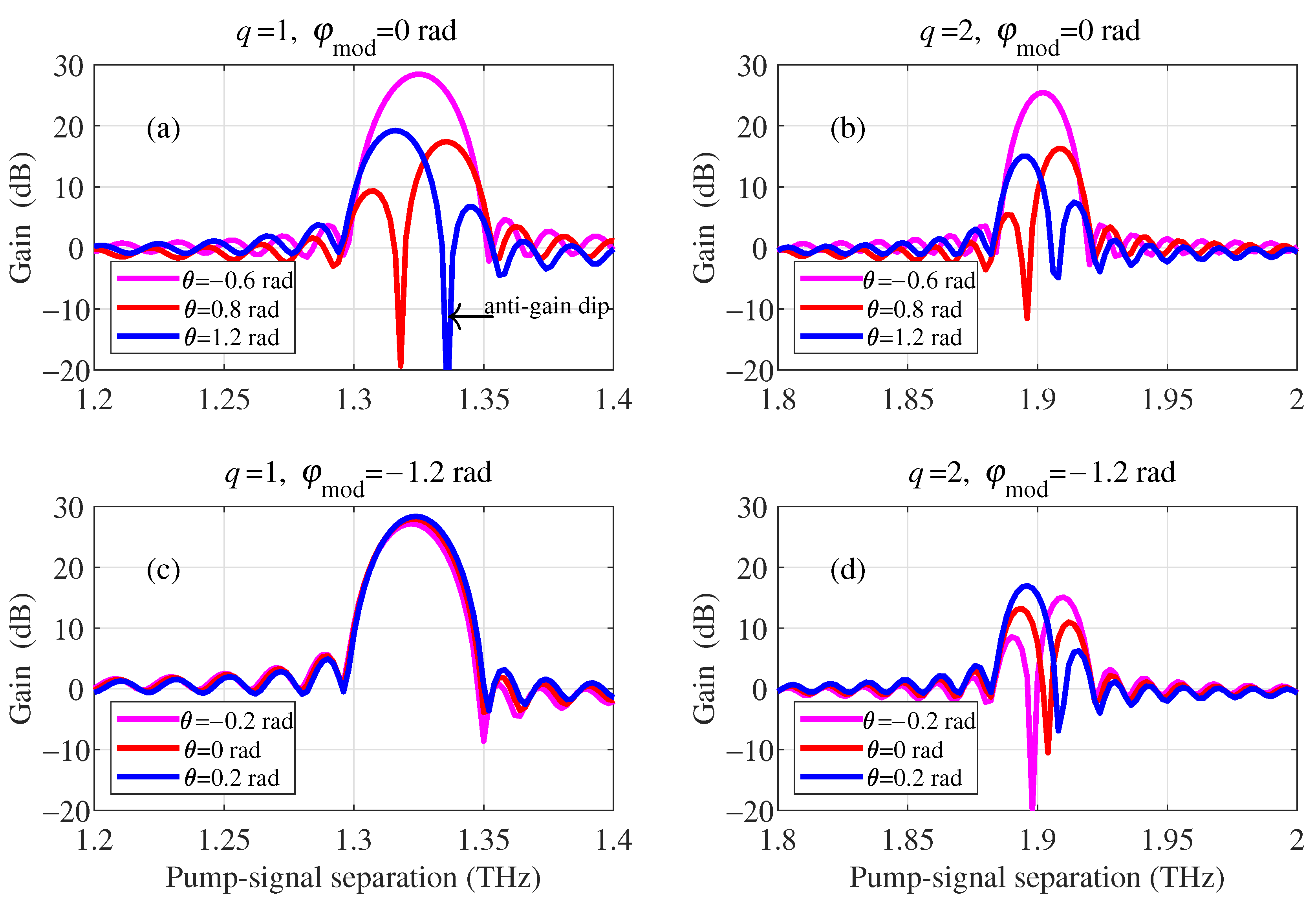
In this section we focus on a single pump configuration. Single pump configurations are often simpler in terms of theoretical treatment since they do not contain high-order pumps that are generated through cascaded four-wave mixing between the pumps in a dual pump configuration [42,43].

Considering the Taylor series expansion of $\beta \left(\omega \right)$ till the $2p$-order, the linear phase mismatch (9) is given by:

$$\xi \left(z\right)=\sum _{k=1}^p\frac{2{\Omega }_{ps}^{2k}}{\left(2k\right)!}{\int }_0^z{\beta }_{2k}\left(z^{\prime }\right)d{z}^{\prime },$$

(10)

where ${\beta }_{2k}\left(z\right)$ are even coefficients of the Taylor series expansion of $\beta \left(\omega \right)$. Integrating Equation (5), we get

$$\xi \left(z\right)=\sum _{k=1}^p\frac{2{\Omega }_{ps}^{2k}}{\left(2k\right)!}\left\{{\overline{\beta }}_{2k}z-{\tilde{\beta }}_{2k}\frac{z_{\mathrm{mod}}}{2\pi }\left[cos\left(\frac{2\pi z}{z_{\mathrm{mod}}}+{\phi }_{\mathrm{mod}}\right)-cos\left({\phi }_{\mathrm{mod}}\right)\right]\right\}.$$

(11)

In Equations (7) and (8) the amplitudes $A_{-1}$, $A_1$, and $A_0$ correspond to idler, signal and pump waves. We can analyze Equations (7) and (8) by assuming that the pump power $P_0={\left|A_0\right|}^2$ is much larger than the power of signal and idler. In a lossless assumption $(\alpha =0)$, the amplitude of the pump can be written as $A_0\left(z\right)=a_{0}exp\left(i\gamma P_{0}z\right)$. We then insert this into Equation (8), and substitute $A_{\pm 1}\left(z\right)=a_{\pm 1}\left(z\right)exp[i\gamma P_{0}z-iz{\sum }_{k=1}^p{\overline{\beta }}_{2k}{\Omega }_{ps}^{2k}{(\left(2k\right)!)}^{-1}]$ to obtain coupled equations:

$$\begin{array}{ccc}\hfill \frac{d{a}_1}{dz}& =& i{a}_1\left(\gamma P_0+\sum _{k=1}^p\frac{{\overline{\beta }}_{2k}{\Omega }_{ps}^{2k}}{\left(2k\right)!}\right)+i\gamma a_0^2{a}_{-1}^{*}R\left(z\right)\hfill \end{array}$$

(12)

$$\begin{array}{ccc}\hfill \frac{d{a}_{-1}^{*}}{dz}& =& -i{a}_{-1}^{*}\left(\gamma P_0+\sum _{k=1}^p\frac{{\overline{\beta }}_{2k}{\Omega }_{ps}^{2k}}{\left(2k\right)!}\right)-i\gamma a_0^{*2}{a}_1{R}^{*}\left(z\right),\hfill \end{array}$$

(13)

where

$$R\left(z\right)=exp\left(i\frac{z_{\mathrm{mod}}}{2\pi }\sum _{k=1}^p\frac{2{\tilde{\beta }}_{2k}{\Omega }_{ps}^{2k}}{\left(2k\right)!}\left[cos\left(\frac{2\pi z}{z_{\mathrm{mod}}}+{\phi }_{\mathrm{mod}}\right)-cos\left({\phi }_{\mathrm{mod}}\right)\right]\right).$$

(14)

We expand the function $R\left(z\right)$ as a Fourier series with fundamental period $z_{\mathrm{mod}}$

$$R\left(z\right)=\sum _{q=-\infty }^{\infty }{c}_{q}exp\left(iq\frac{2\pi }{z_{\mathrm{mod}}}z\right),$$

(15)

$$c_q=J_q\left(\frac{z_{\mathrm{mod}}}{2\pi }\sum _{k=1}^p\frac{2{\tilde{\beta }}_{2k}{\Omega }_{ps}^{2k}}{\left(2k\right)!}\right)exp\left(-i\frac{z_{\mathrm{mod}}}{2\pi }\sum _{k=1}^p\frac{2{\tilde{\beta }}_{2k}{\Omega }_{ps}^{2k}}{\left(2k\right)!}cos\left({\phi }_{\mathrm{mod}}\right)+iq\left({\phi }_{\mathrm{mod}}+\frac{\pi }{2}\right)\right),$$

(16)

where $J_q$ are Bessel functions of the first kind.

We introduce $b_{\pm 1}\left(z\right)=a_{\pm 1}\left(z\right)exp(-iq\pi z/z_{\mathrm{mod}})$. Then equating the coefficients of $exp(-iq\pi z/z_{\mathrm{mod}})$ gives

$$\begin{array}{ccc}\hfill \frac{d{b}_1}{dz}& =& i\kappa b_1+i\chi b_{-1}^{*},\hfill \end{array}$$

(17)

$$\begin{array}{ccc}\hfill \frac{d{b}_{-1}^{*}}{dz}& =& -i{\chi }^{*}{b}_1-i\kappa b_{-1}^{*},\hfill \end{array}$$

(18)

where $\chi =\gamma c_q{P}_{0}exp\left(i2\theta \right)$, $\theta =arg\left(a_0\right)$ is the initial phase angle of the pump wave, and

$$\kappa =\gamma P_0+\sum _{k=1}^p\frac{{\overline{\beta }}_{2k}{\Omega }_{ps}^{2k}}{\left(2k\right)!}-q\frac{\pi }{z_{\mathrm{mod}}}.$$

(19)

The solution of Equations (17) and (18) can be written as

$$\begin{array}{ccc}\hfill b_1\left(z\right)& =& \mu b_1\left(0\right)+\nu b_{-1}^{*}\left(0\right),\hfill \end{array}$$

(20)

$$\begin{array}{ccc}\hfill b_{-1}^{*}\left(z\right)& =& {\nu }^{*}{b}_1\left(0\right)+{\mu }^{*}{b}_{-1}^{*}\left(0\right),\hfill \end{array}$$

(21)

where $\mu \left(z\right)=cosh\left(gz\right)+i\kappa g^{-1}sinh\left(gz\right)$, and $\nu \left(z\right)=i\chi g^{-1}sinh\left(gz\right)$. Here the parametric gain coefficient

$$g={\left(\right|\chi |}^2-{\kappa }^2{)}^{1/2}=\left[\right(\gamma P_0|c_q{\left|\right)}^2-{\kappa }^2{]}^{1/2}.$$

(22)

For the fundamental band $(q=0)$, expression for the gain coefficients (22) represents conventional parametric gain in optical fibers [5,35,44].

In assumption that the idler and signal input powers are equal $\left(\right|b_1\left(0\right){|}^2=\left|b_{-1}\left(0\right){|}^2\right)$, the total gain for q-th component of the signal wave can be calculated as follows

$$G_q\left(z\right)=\frac{|b_{-1}{\left(z\right)|}^2}{|b_{-1}{\left(0\right)|}^2}={\left|\mu \right|}^2+{\left|\nu \right|}^2+2\left|\mu \right|\left|\nu \right|cos\left({\Phi }_q\right),$$

(23)

where ${\Phi }_q=arg\left(b_1\left(0\right)b_{-1}\left(0\right)\mu {\nu }^{*}\right)={\phi }_1+{\phi }_{-1}+{\phi }_{\mu }-{\phi }_{\nu }$. Here ${\phi }_{\pm 1}=arg\left(b_{\pm 1}\left(0\right)\right)=arg\left(A_{\pm 1}\left(0\right)\right)$ are initial phase angles for the signal and idler waves, ${\phi }_{\mu }=arctan(g^{-1}\kappa tanh\left(gz\right))$ is the phase angle of the complex function $\mu \left(z\right)$, and ${\phi }_{\nu }=arg\left(\nu \right)$ is the phase angle of the complex function $\nu \left(z\right)$. Expression for ${\Phi }_q$ can be rewritten in the following form

$${\Phi }_q={\phi }_{\mu }+\frac{z_m}{2\pi }\sum _{k=1}^p\frac{2{\tilde{\beta }}_{2k}{\Omega }_{ps}^{2k}}{\left(2k\right)!}cos\left({\phi }_{\mathrm{mod}}\right)-\frac{\pi }{2}(q+1)+({\phi }_1+{\phi }_{-1}-2\theta -q{\phi }_{\mathrm{mod}}).$$

(24)

Equations (23) and (24) represent nonlinear interference of the signal and idler. The interference is phase-sensitive, and the signal and idler can interfere constructively and destructively. The total gain of the signal wave (23) has maximum for ${\Phi }_q=0$ (parametric amplification) and minimum for ${\Phi }_q=\pi$ (parametric attenuation). By having signal, idler, and pump waves present at the fiber input and adjusting the relative phase between them, we are able to adjust signal amplification. A remarkable feature of the PSA in the DOF is the dependence of the relative phase ${\Phi }_q$ on the modulation phase of the fiber dispersion ${\phi }_{\mathrm{mod}}$. This feature will be discussed in the Section 3.2.

Let us consider the total gain the signal wave when the initial idler is zero, $b_1\left(0\right)=0$. From (20) we can find that the idler wave is proportional to the conjugated signal, namely ${\phi }_1=-{\phi }_{-1}+{\phi }_{\nu }$. The gain of the signal wave $G_q={\left|\mu \right|}^2$ does not depend on the phases ${\phi }_1$, ${\phi }_{-1}$, $\theta$, and ${\phi }_{\mathrm{mod}}$. In other words, in presence only two input waves we have phase-insensitive amplification.

The highest gain occurs for phase-matching condition $\kappa =0$, see Equation (22). The frequency detuning ${\Omega }_q$ corresponding to the largest gain coefficient can be found from a polynomial expression:

$$q\frac{\pi }{z_{\mathrm{mod}}}-\gamma P_0=\sum _{k=1}^p\frac{{\overline{\beta }}_{2k}{\Omega }_q^{2k}}{\left(2k\right)!}$$

(25)

An approximative transformation of Equation (25) may be done from the frequency domain to the more generally used wavelength domain [44]. Derivatives ${\overline{\beta }}_{2k}$ are calculated for the frequency of the pump wave ${\omega }_0=2\pi c{\lambda }_p^{-1}$, where ${\lambda }_p^{-1}$ is the pump wavelength. We can calculate dispersion coefficients ${\overline{\beta }}_{2k+1}^{\mathrm{zero}}=d^{2k+1}\overline{\beta }/d{\omega }^{2k+1}$ at the frequency ${\omega }_{\mathrm{zero}}=2\pi c{\lambda }_{\mathrm{zero}}^{-1}$ corresponding to the zero-dispersion wavelength ${\lambda }_{\mathrm{zero}}$. In assumption, that the dispersion coefficients increase linearly with the frequency, i.e., ${\overline{\beta }}_{2k}={\overline{\beta }}_{2k+1}^{\mathrm{zero}}({\omega }_0-{\omega }_{\mathrm{zero}})$, Equation (25) becomes

$$q\frac{\pi }{z_{\mathrm{mod}}}-\gamma P_0=-2\pi c\frac{{\lambda }_p-{\lambda }_{\mathrm{zero}}}{{\lambda }_p{\lambda }_{\mathrm{zero}}}\sum _{k=1}^p\frac{{\overline{\beta }}_{2k+1}^{\mathrm{zero}}}{\left(2k\right)!}\frac{{\left[2\pi c({\lambda }_p-{\lambda }_s)\right]}^{2k}}{{\left({\lambda }_p{\lambda }_s\right)}^{2k}},$$

(26)

where ${\lambda }_s=2\pi c/{\omega }_{-1}$ is the wavelength of the signal wave. The parametric gain coefficient g depends on the pump power $P_0$ and average dispersion coefficients.

The analytical treatment of expressions (25) and (26) in the presence of high-order dispersion terms is quite complicated. However, we can find that phase-matching can be achieved both in regime of anomalous average dispersion $({\lambda }_p>{\lambda }_{\mathrm{zero}})$ and in regime of normal average dispersion $({\lambda }_p<{\lambda }_{\mathrm{zero}})$. The sign of the right side of Equation (26) depends on the impact of the high-order dispersion terms. The left side of Equation (26) can be positive or negative, as the integer q can take on both positive and negative values. As a result, the phase-matching (26) can be satisfied with the appropriate sign of q. To demonstrate the formation of the gain sidebands in regime of the normal and anomalous average dispersion we calculate the gain of the signal wave $G_S$ (Figure 4) as

$$G_S=\frac{|A_{-1}{\left(L\right)|}^2}{|A_{-1}{\left(0\right)|}^2},$$

(27)

where $L=1.4$ km is the fiber length, $A_{-1}\left(L\right)$ is calculated numerically from Equations (7) and (8). We use the Taylor expansion of $\beta \left(\omega \right)$ up to the fourth order. The modulation period is $z_m=40$ m, and the effective nonlinearity is $\gamma =9.44$ (W km)⁻¹. The attenuation coefficient is assumed $\alpha =0.092 {\mathrm{km}}^{-1}$, which corresponds to 0.4 dB/km. Figure 4a shows the parametric gain in the regime of the anomalous average dispersion. To provide consistency between the analytical results and numerical simulations, q must be assigned negative values. For the description of the gain in the normal average dispersion (Figure 4b) we have to use in the analytical model the positive integer q. The analytical three-wave model agrees well with the numerical solution of the full system given by Equations (7) and (8). The model accurately describes the line shapes of the gain. Figure 4c shows the gain in the fifth sideband, $q=5$. The analytical model do not consider the pump depletion. Due to this feature, the parametric gain $G_q$ is overestimated (Figure 4c).

3.2. Role of Pump Phase $\theta$ and Modulation Phase ${\phi }_{\mathit{mod}}$ on Signal Gain

To demonstrate the effect of the dispersion oscillation on the PSA we solve Equations (7) and (8) numerically. In these calculations, we assume that the initial power of the pump wave $P_0$ to be $0.5 \mathrm{W}$. The initial powers of the signal and idler waves are $|A_{-1}{\left(0\right)|}^2={\left|A_1\left(0\right)\right|}^2={10}^{-6} \mathrm{W}$. Since for a PSA, the total gain depends on the common phase $({\phi }_1+{\phi }_{-1}-2\theta -q{\phi }_{\mathrm{mod}})$ (see Equations (23) and (24)), the signal and idler phases at the input of the fiber are considered to be zero. Simulations are carried out for different input pump phase $\theta$ and modulation phase ${\phi }_{\mathrm{mod}}$. The dispersion modulation profile of the considered DOF with single modulation frequency follow Equation (5).

In the case of PSA in DOFs, the high-order sidebands ($q\ne 0$) provide interesting perspectives in terms of applications. To evaluate the signal gain $G_S$ we scan the pump-signal frequency separation near the two resonant frequencies ${\nu }_1$ and ${\nu }_2$ (i.e., $q=1$ and 2), for different input phases $\theta$ and different dispersion modulation phases ${\phi }_{\mathrm{mod}}$ (see Figure 5). At $\theta =-0.6$ rad, a broadband amplification peak is observed. A change in the phase of the pump wave leads to the emergence of a narrow parametric attenuation gap (anti-gain dip) with a high extinction of about 30 dB [see Figure 5a]. As the phase is varied from $\theta =-0.6$ rad to $\theta =1.2$ rad, the anti-gain dip moves through the gain spectrum from low to high frequency pump signal separation. The dip’s shift occurs synchronously for both the first $(q=1)$ and second $(q=2)$ gain band. This is an interesting feature of the PSA system that would allow preferentially filtering out unwanted frequencies in a wavelength multiplexed system, just by tuning the phase of the input signal.

Contrary to a phase insensitive amplification with a DOF [12], we further found out that the position of the anti-gain dip depends not only on the phase of the pump wave $\theta$, but also on the phase of the dispersion modulation ${\phi }_{\mathrm{mod}}$. From Figure 5c,d, we see that for the modulation phase ${\phi }_{\mathrm{mod}}=-1.2$ rad the first band ($q=1$) remains unaffected as the modulation phase is increased from $\theta =-0.2$ rad to $\theta =0.2$ rad. At the same conditions the second band ($q=2$) show the characteristic dip in the gain spectrum.

The behavior of anti-gain dip can be explained using the analytical model given in Section 3.1. The gain bandwidth of the q-th spectral component is given by the frequency dependency of the gain coefficient (22). The parametric attenuation within selected q-th band is realized under the condition $cos\left({\Phi }_q\right)=-1$ in Equation (23). The value of ${\Phi }_q$ depends on the phases as $({\phi }_1+{\phi }_{-1}-2\theta -q{\phi }_{\mathrm{mod}})$. This value does not depends on the q when ${\phi }_{\mathrm{mod}}=0$. As a result, anti-gain dips appear in the first $(q=1)$ and second $(q=2)$ bands synchronously (Figure 5a,b). Effect of the harmonic number q on the condition $cos\left({\Phi }_q\right)=-1$ appears only for nonzero ${\phi }_{\mathrm{mod}}$. When ${\phi }_{\mathrm{mod}}=-1.2$ rad the condition $cos\left({\Phi }_q\right)=-1$ is not reached within the first band $(q=1)$ (Figure 5c). The first band remains unchanged for $\theta =-0.2,0$, and $0.2$ radians. While for the second band $(q=2)$, the frequency corresponding to the condition $cos\left({\Phi }_q\right)=-1$ moves across the entire band (Figure 5d).

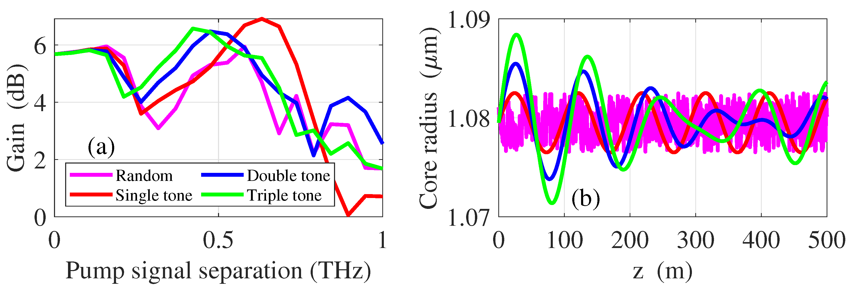
3.3. DOF with Multiple Frequency of Dispersion Modulation

One impediment to the use of the high-order gain sidebands of a DOF-based PSA for amplification purposes is its narrow bandwidth. However, using of multiple closely spaced frequencies of dispersion modulation can alleviate this restriction to some degree [18]. Note that different dispersion modulation frequencies will inevitably have their individual gain band centers at different frequencies and hence the combined effect will lead to a wider gain band. Thus we consider the case where modulation of the fiber core diameter is given by a superposition of three sinusoidal functions:

$$a\left(z\right)=\overline{a}+{\tilde{a}}_{1}sin\left(\frac{2\pi }{z_{m1}}z\right)+{\tilde{a}}_{2}sin\left(\frac{2\pi }{z_{m2}}z-1.1\right)+{\tilde{a}}_{3}sin\left(\frac{2\pi }{z_{m3}}z\right),$$

(28)

where $\overline{a}=2.1 \mathsf{\mu }$m, ${\tilde{a}}_1=0.08 \mathsf{\mu }\mathrm{m}$, ${\tilde{a}}_2=0.1 \mathsf{\mu }\mathrm{m}$, ${\tilde{a}}_3=0.04 \mathsf{\mu }\mathrm{m}$, $z_{m1}=40$ m, $z_{m2}=40.5$ m, and $z_{m3}=41.5$ m. The amplitudes and phases of the sine functions are selected so as to provide a uniform amplification in the band from ${\Omega }_{ps}{\left(2\pi \right)}^{-1}=1.28$ THz to ${\Omega }_{ps}{\left(2\pi \right)}^{-1}=1.32$ THz. The corresponding calculated dispersion parameters are shown in Figure 6a.

Figure 6b,c show the signal gains calculated for $q=1$ and $q=2$ respectively for multi-frequency modulation for different pump input phases. For $q=1$, the gain bandwidth is found to be 40 GHz with a gain ripple of 1 dB for $\theta =2$ rad. This is a significant improvement over the DOF with a single dispersion modulation frequency [see Figure 5a,c] where the gain bandwidth was 22 GHz. Nevertheless, an increase in bandwidth for the multi-frequency modulation is accompanied by a decrease in the peak gain of about 15 dB.

To investigate this further we plot in Figure 7 the full gain spectrum dependence of the system on the input pump phase $\theta$ for $q=1$ and $q=2$. The signal gain is found to be a periodic function of $\theta$, as is expected in a traditional PSA. The positive and negative gains with an extinction of about 24 dB indicate a strong squeezing of the signal and idler modes [45]. While for $q=1$, the peak of the gain band corresponds to $\theta =-1\pm \pi ,-1\pm 2\pi ,\dots$, for $q=2$ the peak gain corresponds to a different value ${\phi }_0=-1.87\pm \pi ,-1.87\pm 2\pi ,\dots$. This feature of the gain profile is associated with the dependence of the gain on the modulation phase of the different dispersion modulation components.

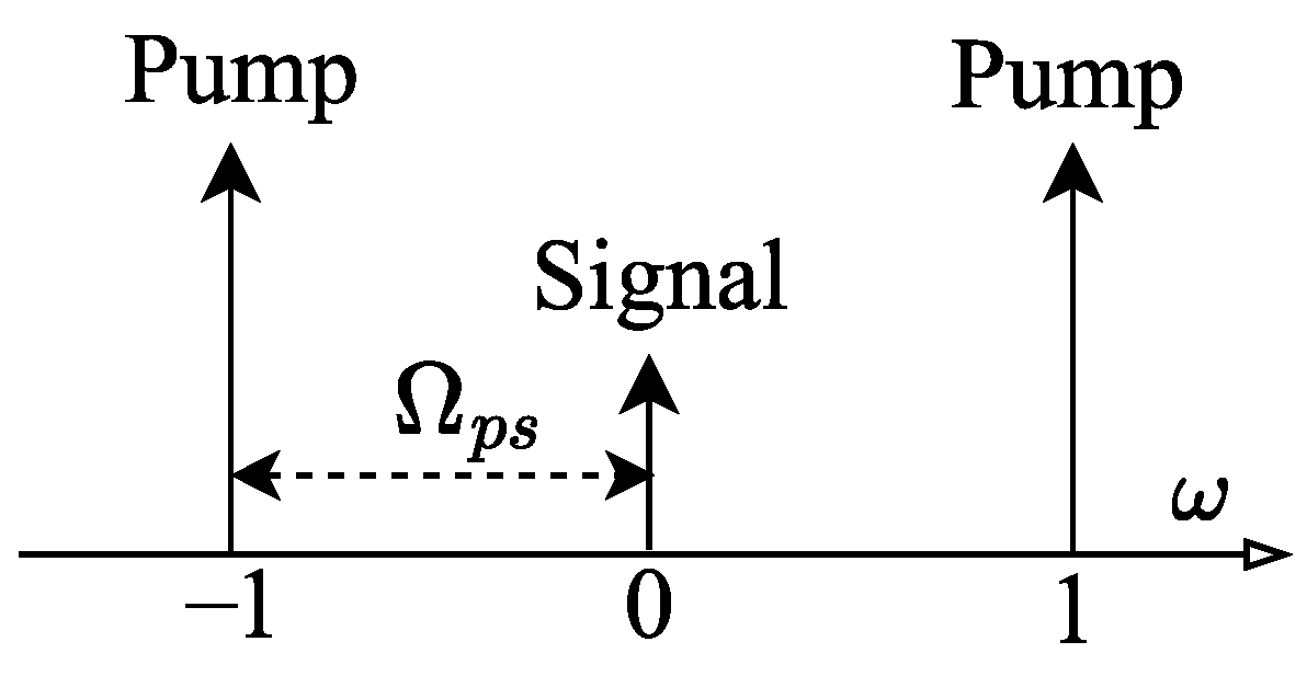
4. PSA in a DOF: Dual Pump Configuration

In the preceding section, we focused on a single pump PSA system with a DOF. However, a dual pump PSA system is often preferred to a single pump system, owing to its ability to provide a larger gain [46], or for the amplification of polarization multiplexed optical signals [47,48]. Since here our focus will be on achieving a larger gain for the PSA system, we will restrict our discussion to the fundamental gain band ($q=0$) of the system, that typically can reach gains much larger than the high-order sidebands [49].

In this section we aim to optimize the dispersion modulation parameters of the DOF, such that a high PSA gain can be attained. To this aim, we first introduce an analytical model for a dual-pump PSA considering dispersion oscillation. The dual pump system configuration is illustrated in Figure 8.

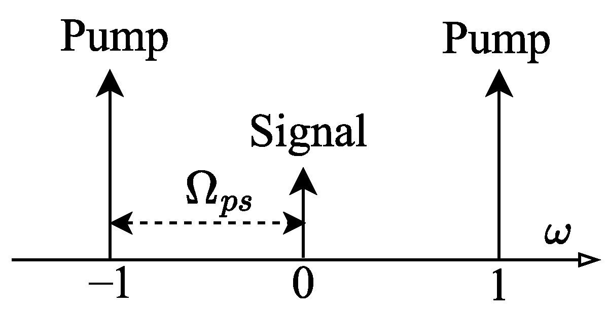
4.1. Analytical Model: Three Wave Approach

In this section we describe the standard three-wave (two pumps and a degenerate signal) model [23] for studying the signal gain in a DOF. In this model we neglect the fiber attenuation and consider the pumps to be undepleted along the length of the fiber. We also set the phase of the dispersion modulation ${\phi }_{\mathrm{mod}}=0$ rad.

The differential equations governing the evolution of the signal and the two pumps are Equation (7) and Equation (8) respectively. Setting $\alpha =0$ in Equation (8) and considering the two pumps to be undepleted along the length of the DOF, their slowly varying complex amplitudes denoted by $A_{\pm 1}$ are given by:

$$A_{\pm 1}=\sqrt{P}{e}^{i3\gamma Pz},$$

(29)

where P is the undepleted pump power. Here we assumed the input phases of the pumps to be 0 rad. Using Equation (29) in Equation (7), and considering the pump waves to be much stronger than the signal, hence neglecting self-phase modulation, the evolution of the slowly varying complex amplitude of the signal $A_0\left(z\right)$ is thus given by:

$$\frac{d{A}_0}{dz}=i2\gamma P\left[2A_0+A_0^{*}{e}^{i6\gamma Pz}{e}^{i\xi \left(z\right)}\right].$$

(30)

Considering Equation (10) for ${\phi }_{\mathrm{mod}}=0$ and ${\overline{\beta }}_j=0$, $j=4,6,\dots$, we get:

$$\xi \left(z\right)={\Omega }_{ps}^2\left[{\overline{\beta }}_{2}z-\widetilde{{\beta }_2}\frac{z_{\mathrm{mod}}}{2\pi }cos\left(\frac{2\pi z}{z_{\mathrm{mod}}}\right)+\frac{\widetilde{{\beta }_2}{z}_{\mathrm{mod}}}{2\pi }\right].$$

(31)

We note from the above expression that the dispersion oscillation can only have a non-negligible effect only when ${\tilde{\beta }}_2$ is much larger than ${\overline{\beta }}_2$. This is typically the case for ${\overline{\beta }}_2\approx 0$. One might argue that when ${\overline{\beta }}_2\approx 0$, the high order dispersion terms neglected in the Taylor series expansion of ${\beta }_2$ might have a significant impact on the gain dynamics. But, we should also remember that in our case ${\overline{\beta }}_2\approx 0$ does not mean that ${\beta }_2\approx 0$ throughout the fiber length, since ${\beta }_2$ depends on z. In fact, there are only few (as many as the number of cycles of the dispersion oscillation) regions in the fiber where ${\beta }_2\approx 0$. In all the other regions, the absolute local value of ${\beta }_2$ is larger, which depends on ${\tilde{\beta }}_2$. Numerical simulations are utilized to validate this assumption, as we discuss later. Using Equation (31) in Equation (30), the evolution of $A_0$ is given by:

$$\begin{array}{cc}\hfill & \frac{d{A}_0}{dz}=i\gamma P[4A_0+2A_0^{*}exp\left(i6\gamma Pz+i{\Omega }_{ps}^2{\overline{\beta }}_{2}z+\frac{i{\Omega }_{ps}^2\widetilde{{\beta }_2}{z}_{\mathrm{mod}}}{2\pi }\right)\hfill \\ \hfill & \times \sum _{n=-\infty }^{\infty }{i}^n{J}_n\left(\frac{-{\Omega }_{ps}^2\widetilde{{\beta }_2}{z}_{\mathrm{mod}}}{2\pi }\right)exp\left(\frac{i2\pi nz}{z_{\mathrm{mod}}}\right)],\hfill \end{array}$$

(32)

where $J_n\left(\right)$ is the Bessel function of the first kind, of order n. Here we have used the Jacobi-Anger expansion, to convert the cosine in the exponential term in Equation (30) into an infinite series of exponentials with linear exponents. In order to solve for $A_0$, we perform the following transformation of variable:

$$A_0=B_{q}exp\left[i\left(3\gamma P+\frac{{\overline{\beta }}_2{\Omega }_{ps}^2}{2}+\frac{q\pi }{z_{\mathrm{mod}}}\right)z+\frac{i{\Omega }_{ps}^2\widetilde{{\beta }_2}{z}_{\mathrm{mod}}}{4\pi }\right],$$

(33)

where $q\in \mathbb{Z}$ is a parameter that corresponds to the DOF induced sideband order [17]. Thus Equation (32) can be written as:

$$\frac{d{B}_q}{dz}=i\gamma P\left[\left(1-\frac{{\overline{\beta }}_2{\Omega }_{ps}^2}{2\gamma P}-\frac{q\pi }{\gamma P{z}_{\mathrm{mod}}}\right)B_q+2B_q^{*}\sum _{n=-\infty }^{\infty }{i}^n{J}_n\left(-\frac{{\Omega }_{ps}^2\widetilde{{\beta }_2}{z}_{\mathrm{mod}}}{2\pi }\right)exp\left(\frac{i2\pi (n-q)z}{z_{\mathrm{mod}}}\right)\right].$$

(34)

At this point, to get rid of the infinite series in Equation (34), we make the following approximation. We note that the effective contribution of the oscillating terms in the series, over large propagation distances ($z\gg z_{\mathrm{mod}}$) is negligible. However, the only terms that are not oscillating, appear when $n=q$ [14]. Thus neglecting the terms with $n\ne q$ in Equation (34), the q-th order state column vector ${\mathbf{B}}_q\left(z\right)={\left[\begin{array}{cc}{B}_q& {B_q}^{*}\end{array}\right]}^{\mathrm{T}}$ can be written in a matrix form as:

$$\frac{d{\mathbf{B}}_q}{dz}={\mathbf{M}}_q{\mathbf{B}}_q,$$

(35)

where ${\mathbf{M}}_q$ is the coefficient matrix for the ordinary differential equation (ODE) system, given by:

$${\mathbf{M}}_q=i\gamma P\left[\begin{array}{cc}\left(1-\frac{{\overline{\beta }}_2{\Omega }_{ps}^2}{2\gamma P}-\frac{q\pi }{\gamma P{z}_m}\right)& 2e^{\frac{q\pi }{2}}{J}_q\left(-\frac{{\Omega }_{ps}^2\widetilde{{\beta }_2}{z}_m}{2\pi }\right)\\ -2e^{\frac{-q\pi }{2}}{J}_q\left(-\frac{{\Omega }_{ps}^2\widetilde{{\beta }_2}{z}_m}{2\pi }\right)& -\left(1-\frac{{\overline{\beta }}_2{\Omega }_{ps}^2}{2\gamma P}-\frac{q\pi }{\gamma P{z}_m}\right)\end{array}\right].$$

(36)

The solution of ${\mathbf{B}}_q\left(z\right)$ can be obtained through the matrix exponential method [5], and is given by:

$${\mathbf{B}}_q\left(z\right)=\left[cos\left(gz\right)\mathbf{I}+\frac{sin\left(gz\right)}{g}{\mathbf{M}}_q\right]{\mathbf{B}}_q\left(0\right)={\mathbf{T}}_q\left(z\right){\mathbf{B}}_q\left(0\right),$$

(37)

where $\mathbf{I}$ is 2 × 2 identity matrix, ${\mathbf{T}}_q\left(z\right)$ is the transfer matrix that transforms state ${\mathbf{B}}_q\left(0\right)$ into ${\mathbf{B}}_q\left(z\right)$, and the parametric gain coefficient g [50] is given by:

$$\begin{array}{cc}\hfill g=& \gamma P{\left[{\left(1-\frac{{\overline{\beta }}_2{\Omega }_{ps}^2}{2\gamma P}-\frac{q\pi }{\gamma P{z}_{\mathrm{mod}}}\right)}^2-4J_q{\left(\frac{-{\Omega }_{ps}^2\widetilde{{\beta }_2}{z}_{\mathrm{mod}}}{2\pi }\right)}^2\right]}^{\frac{1}{2}}.\hfill \end{array}$$

(38)

From the above expression of g in Equation (38) we notice that g can be either real or imaginary depending on the balance between the first and the second term. As a consequence, when g is imaginary, the sines and cosines in Equation (37) turn hyperbolic sines and cosines leading to exponential, or in other words high gain situations.

It is easily proven that ${\mathbf{T}}_q\left(z\right)$ has a unity determinant. Thus ${\mathbf{T}}_q\left(z\right)$ is a symplectic matrix. We also note here that ${\mathbf{T}}_q\left(z\right)$ has the same form of a transfer matrix of a standard two-mode squeezed state arising from a fiber phase sensitive amplifier [45].

We are typically interested in the case of $q=0$, or in other words the fundamental gain band of the modulation instability (MI) spectrum of a DOF [14]. As a sanity check, putting $q=0$ (for the fundamental gain band) and ${\tilde{\beta }}_2=0$ (meaning no dispersion oscillation) in Equation (38) gives us:

$$g=\gamma P{\left[-3-\frac{{\overline{\beta }}_2{\Omega }_{ps}^2}{\gamma P}+{\left(\frac{{\overline{\beta }}_2{\Omega }_{ps}^2}{2\gamma P}\right)}^2\right]}^{\frac{1}{2}},$$

(39)

which is the parametric gain coefficient for a standard HNLF in a dual-pump configuration with a degenerate signal [43].

The analytical results of the maximum PSA signal gain in the fundamental gain band ($q=0$) for a DOF of length $L=1000$ m, pump power $P=22$ dBm, $z_{\mathrm{mod}}=250$ m and $\gamma =4$ (W km)⁻¹ and 10 (W km)⁻¹ are plotted in Figure 9g,h,i and Figure 10g,h,i respectively. Three different values of ${\overline{\beta }}_2$ were considered, i.e., −5 ps²/km, 0 ps²/km, and 5 ps²/km, corresponding to left, middle and right columns respectively.

Since in this model, the high-order waves generated in the DOF, pump depletion, as well as the high-order ${\beta }_m$’s were ignored, it is necessary to compare the analytical results with numerical calculation based on the nonlinear Schrödinger equation (NLSE) that is immune to those assumptions.

4.2. Numerical Model: Nonlinear Schrödinger Equation (NLSE)

For an accurate numerical modeling of the propagation of the waves through the dispersion tailored fiber, we resort to the high-order NLSE given by:

$$\frac{\partial A}{\partial z}+\frac{i{\beta }_2\left(z\right)}{2}\frac{{\partial }^{2}A}{\partial T^2}-\frac{{\beta }_3\left(z\right)}{6}\frac{{\partial }^{3}A}{\partial T^3}-\frac{i{\beta }_4\left(z\right)}{24}\frac{{\partial }^{4}A}{\partial T^4}-i\gamma {\left|A\right|}^{2}A=0,$$

(40)

where $A(z,T)$ is the time domain complex amplitude of the wave propagating along z, $T=t-{\beta }_{1}z$ is the retarded time. The variation of ${\beta }_2$, ${\beta }_3$ and ${\beta }_4$ with fiber core radius are modeled as linear functions [24] following the numerical results discussed in Section 2.1. We utilize a split-step Fourier method (SSFM) to solve the NLSE. We consider a frequency resolution of 67 MHz and a space step of size $dz=10$ m. The step size was chosen such that at each step of the SSFM propagation, the accumulated nonlinear phase in the spectrum is much smaller than $\pi$. Thereafter we simulate the output spectrum for different values of pump-signal frequency separation. The maximum PSA gain was obtained by scanning the input signal phase from 0 to $\pi$.

In this work we focus on three principal regions, one with an average dispersion ${\overline{\beta }}_2$, close to 0 ps²/km and the other two around 5 ps²/km and −5 ps²/km. In Figure 11 we show the typical regime of core radius variation, for which a 5 ps²/km variation of ${\beta }_2$ is possible with a W-ratio clamped at 3. The three vertical dashed lines in Figure 11 indicate ${\beta }_2=5$ ps²/km (left), ${\beta }_2=0$ ps²/km (middle) and ${\beta }_2=-5$ ps²/km (right). Thus a core radius variation of 0.1 $\mathsf{\mu }$m would lead to a ${\tilde{\beta }}_2$ of 5 ps²/km.

Consequenctly, the variation in ${\beta }_3$ and ${\beta }_4$ for 1.55 $\mathsf{\mu }$m to 1.65 $\mathsf{\mu }$m core radius variation will be from 35.6 × 10⁻³ ps³/km to 5.7 × 10⁻³ ps³/km, and from 4.4 × 10⁻⁴ ps⁴/km to 2.3 × ${10}^{-4}$ ps⁴/km respectively.

4.3. Profile Optimization for Larger PSA Gain

Here we explore the quest of whether a sinusoidal profile is an optimal profile with respect to providing a large PSA gain as well as reducing SBS due to its varying longitudinal dispersion profile. To this aim, let us first focus our attention in Equation (32). We note that each of the terms in the summation (corresponding to different values of n) at the right hand side of Equation (32) are as if they are different FWM processes. But they give rise to gain peaks at different pump-signal separations since their phase matching condition is different. This is in fact the origin of high-order MI sidebands in DOF based parametric amplifiers [49,51]. But now, let us consider the case where instead of one dispersion oscillation wavelength $z_{\mathrm{mod}}$, there are two, $z_{m1}$ and $z_{m2}$. Note, now ${\beta }_2\left(z\right)$ is given by:

$${\beta }_2\left(z\right)={\overline{\beta }}_2+{\tilde{\beta }}_{2}sin\left(\frac{2\pi z}{z_{m1}}\right)+{\tilde{\beta }}_{2}sin\left(\frac{2\pi z}{z_{m2}}\right).$$

(41)

Thus the linear phase mismatch $\xi \left(z\right)$ becomes:

$$\xi \left(z\right)={\Omega }_{ps}^2\left[{\overline{\beta }}_{2}z-\widetilde{{\beta }_2}\frac{z_{m1}}{2\pi }cos\left(\frac{2\pi z}{z_{m1}}\right)+\frac{\widetilde{{\beta }_2}{z}_{m1}}{2\pi }-\widetilde{{\beta }_2}\frac{z_{m2}}{2\pi }cos\left(\frac{2\pi z}{z_{m2}}\right)+\frac{\widetilde{{\beta }_2}{z}_{m2}}{2\pi }\right].$$

(42)

However, this linear phase mismatch always manifests itself in the exponent as a phase, in the evolution equation of the signal. Thus using the Jacobi-Anger identity, the exponential of $i\xi$ is written as:

$$\begin{array}{cc}\hfill & e^{i\xi \left(z\right)}=\exp \left(i{\Omega }_{ps}^2{\overline{\beta }}_{2}z+\frac{i{\Omega }_{ps}^2\widetilde{{\beta }_2}{z}_{m1}}{2\pi }z+\frac{i{\Omega }_{ps}^2\widetilde{{\beta }_2}{z}_{m2}}{2\pi }\right)\hfill \\ \hfill & \times \left[\sum _{n=-\infty }^{\infty }{i}^n{J}_n\left(\frac{-{\Omega }_{ps}^2\widetilde{{\beta }_2}{z}_{m1}}{2\pi }\right)exp\left(\frac{i2\pi nz}{z_{m1}}\right)\right]\times \left[\sum _{p=-\infty }^{\infty }{i}^p{J}_p\left(\frac{-{\Omega }_{ps}^2\widetilde{{\beta }_2}{z}_{m2}}{2\pi }\right)exp\left(\frac{i2\pi pz}{z_{m2}}\right)\right].\hfill \end{array}$$

(43)

From the above equation it is now clear that in the signal evolution equation, now we will start having inter-modulation tones due to the multiplication between the two infinite series. Thus the gain peaks coming from the fundamental frequencies ($\frac{1}{z_{m1}}$ and $\frac{1}{z_{m2}}$) will be now polluted by the inter-modulation frequencies ($2\frac{1}{z_{m1}}-\frac{1}{z_{m2}}$ and $2\frac{1}{z_{m2}}-\frac{1}{z_{m1}}$) that have a different phase matching condition from the fundamental tones. To illustrate this point we run a numerical NLSE simulation of the system considering different cases, i.e., a constant random profile, a DOF with dispersion oscillation wavelength $z_{m1}$, a profile with $z_{m1}$ and $z_{m2}$ wavelengths and finally a profile with $z_{m1}$, $z_{m2}$ and $z_{m3}$ wavelengths. $z_{m1}=97$ m, $z_{m2}=111$ m and $z_{m3}=122$ m. In Figure 12a we provide the maximum PSA gain as a function of the pump-signal frequency separation and in Figure 12b the corresponding diameter variation along the fiber length is provided. Length of the fiber was 500 m, nonlinear coefficient was 10 (W km)⁻¹, ${\overline{\beta }}_2=1$ ps²/km and pump power was 22 dBm. The maximum PSA gain spectra for these profiles along with the dispersion profiles are shown in Figure 12.

From Figure 12a, we see that when there is only one dispersion oscillation wavelength (red curve), the maximum PSA gain reaches a larger value compared to when two or three wavelengths are present (blue and green curve). In fact, when we use a random profile (magenta curve), it induces even more such wavelengths in the Fourier domain and hence the gain spectrum peak further reduces and starts becoming more uniform and broadened. Similarly, any other non-constant profile will have a large number of frequency components and all these components will lead to a large number of FWM terms and hence would finally compete and bring down the PSA gain spectrum. This same logic also explains the lower peak power and larger bandwidth of the high order gain band in Figure 6 for the single pump PSA case. Therefore, a sinusoidal profile is the most ideal non-constant profile in terms of maximizing the PSA gain.

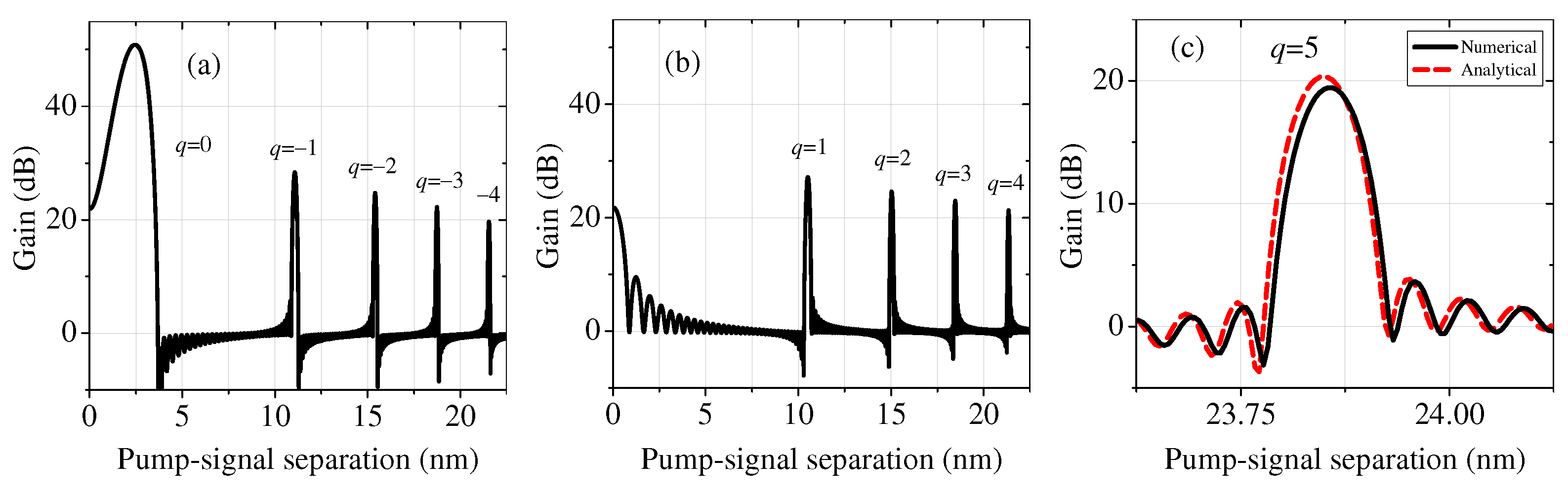
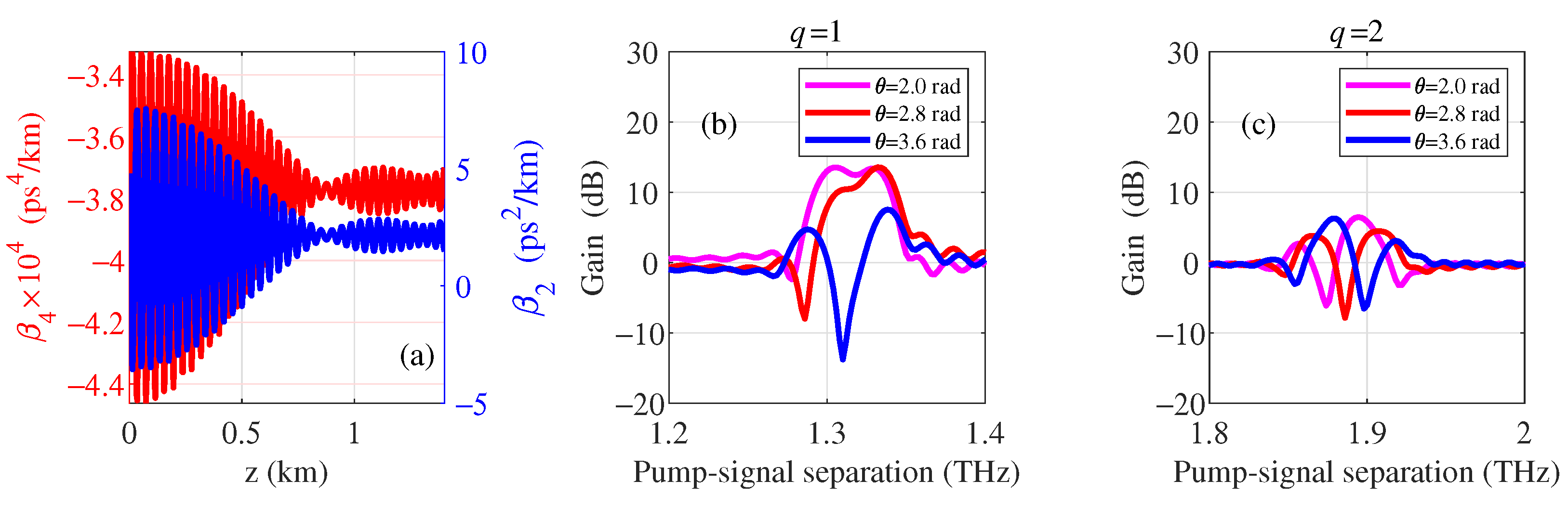
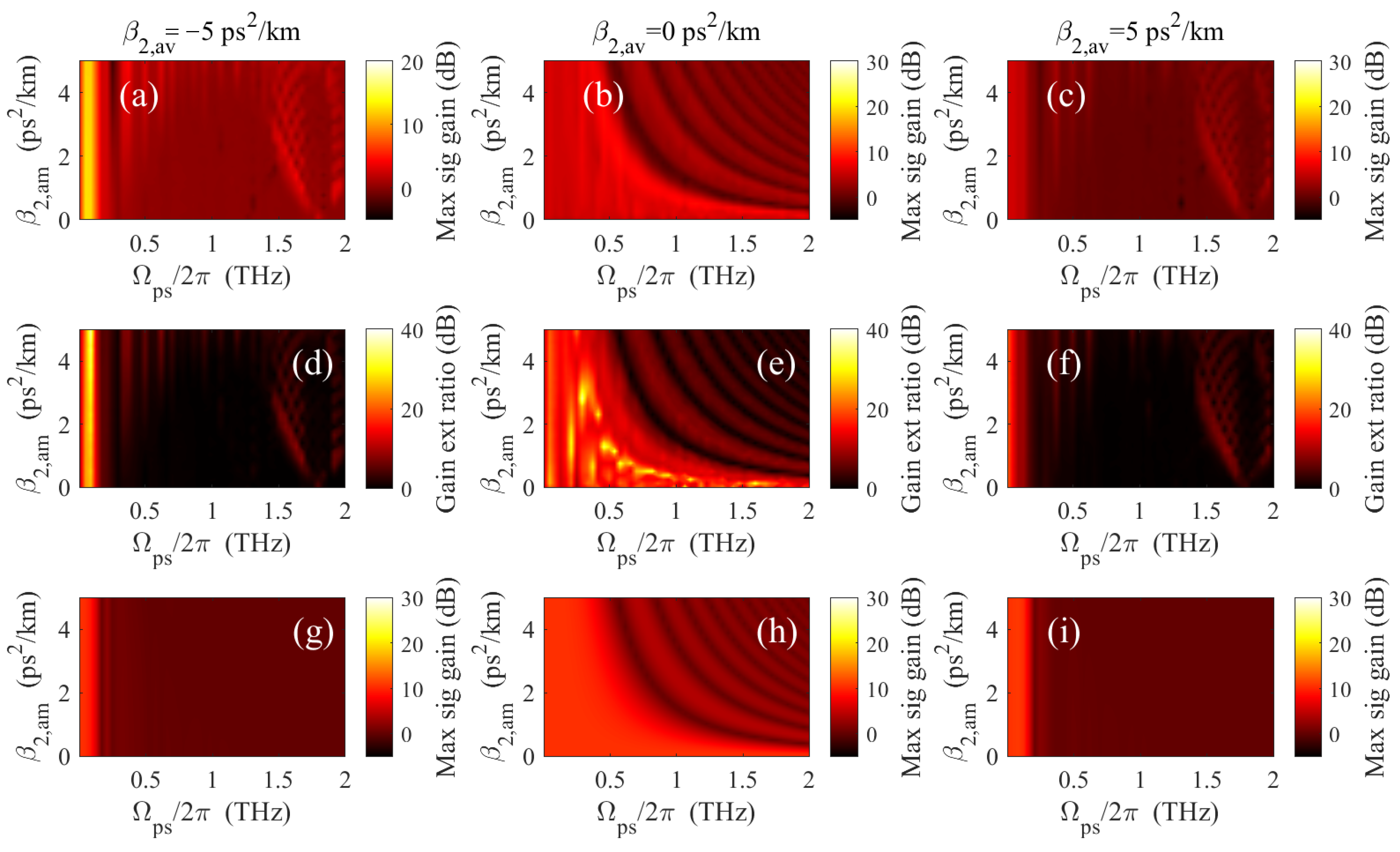
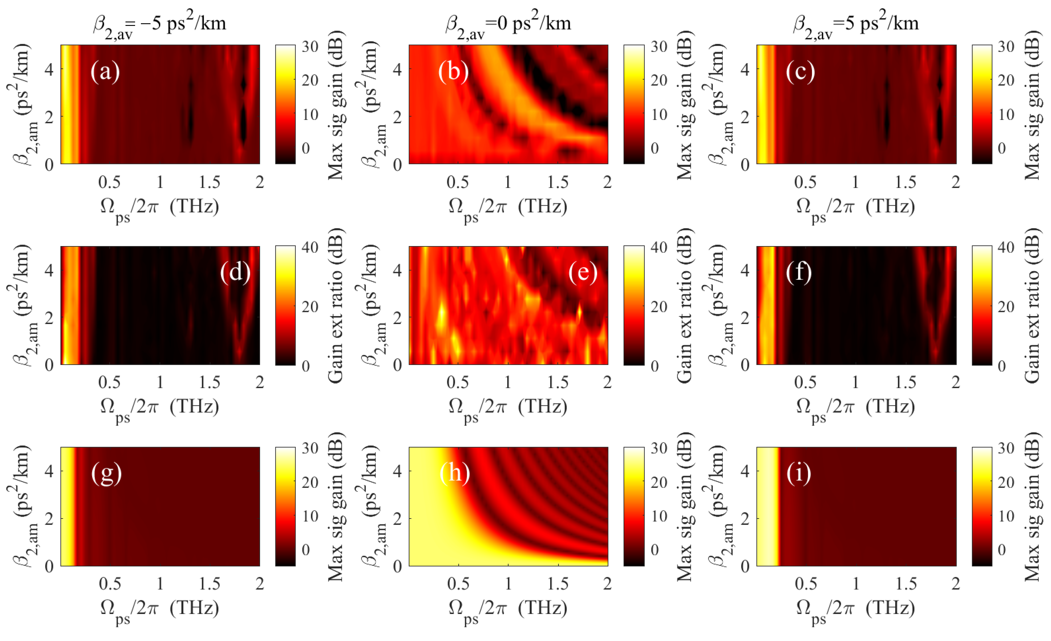
4.4. Numerical Results with Scanning of Dispersion Oscillation Parameters

Having argued that a DOF (with single dispersion modulation frequency) is the best profile for maximizing the PSA gain, here we plot the PSA simulation results, viz, maximum PSA signal gain (top row) and the gain extinction ratio (middle row) in Figure 9 and Figure 10 as false color plots as a function of the pump-signal frequency separation $\frac{{\omega }_{ps}}{2\pi }$, and the amplitude of ${\beta }_2$ oscillation, i.e., ${\tilde{\beta }}_2$. A DOF of length $L=1000$ m, pump power $P=22$ dBm, signal power $P_s=-20$ dBm, period of dispersion oscillation $z_{\mathrm{mod}}=250$ m was considered. $\gamma =4$ (W km)⁻¹ for Figure 9 and 10 (W km)⁻¹ for Figure 10. Three different values of ${\overline{\beta }}_2$ were considered, i.e., −5 ps²/km, 0 ps²/km, and 5 ps²/km, corresponding to the left, middle and right columns respectively.

From Figure 9, firstly we see that the fundamental gain spectrum ($q=0$, or when the pump-signal frequency separation is small, <0.5 THz) is independent of the dispersion oscillation amplitude ${\tilde{\beta }}_2$ for an average ${\overline{\beta }}_2$ away from 0. This is because unless the dispersion oscillation amplitude is large compared to the average dispersion, or more specifically, ${\overline{\beta }}_2$z is comparable to ${\tilde{\beta }}_2\frac{z_{\mathbf{mod}}}{2\pi }$, the effect of dispersion oscillation is negligible as can also be seen from Equation (31). Nevertheless, for ${\overline{\beta }}_2$ away from 0, on increasing ${\tilde{\beta }}_2$, the high-order MI sidebands, corresponding to $q\ne 0$ start to appear [49]. In this case, since the nonlinear phase $\gamma PL$ is about 0.6 rads, the maximum gain of the PSA is about 10 dB. On the contrary, for Figure 10, where the nonlinear phase is about 1.5 rads, the gain is much larger, i.e., above 20 dB. It is also important to note from Figure 10b that a highly flat gain of about 10 dB can be obtained over a large bandwidth of about 1 THz while considering a small $\widetilde{{\beta }_2}\approx 0.4$ ps²/km.

We also note by comparing the top and bottom rows of Figure 9 and Figure 10, that for a low nonlinearity, i.e., when the nonlinear phase is 0.6 rads, the analytical 3-wave model agree satisfactorily with the numerical NLSE model. However, when the nonlinear phase is 1.5 rads, the analytical model predicts a much larger gain than the numerical one for ${\overline{\beta }}_2=-5$ ps²/km and ${\overline{\beta }}_2=5$ ps²/km [43,46]. For ${\overline{\beta }}_2=0$ ps²/km, not only the analytical model overestimates the maximum gain, it also predicts a shorter gain ripple wavelength. This mismatch between the numerical and analytical models is due to the presence of high-order waves that are generated from the FWM processes involving the two strong pumps [49].

5. SBS in a DOF

The aim to achieve a large gain in a PSA relies on the ability to launch large pump powers into the fiber. Stimulated Brillouin scattering (SBS) poses a challenge to this pursuit since it limits the power that can be fed into the fiber. In fact, a high-power pump wave causes a density variation along the fiber’s length that leads to formation of an acoustic wave. This propagating acoustic mode acts as a Bragg grating for the optical wave, resulting in forward and backward scattering. The backward scattered wave, known as the Stokes wave, experiences frequency shifting due to the Doppler effect. The Stokes wave, in turn, reinforces the acoustic wave, leading to further pump scattering and, consequently, a stronger Stokes wave. This nonlinear interaction between the pump, Stokes, and acoustic waves is known as electrostriction [41]. To overcome the problem of SBS, we investigate the SBS dynamics theoretically in this section and outline the implementability of a DOF for SBS mitigation.

5.1. Theory of SBS

The SBS dynamics in a fiber can be mathematically modeled through a set of partial differential equations governing the complex amplitudes of the pump $\mathcal{P}$, Stokes S, and acoustic A waves [41]:

$$\frac{\partial \mathcal{P}}{\partial t}+\frac{c}{n}\frac{\partial \mathcal{P}}{\partial z}=\frac{i\omega {\gamma }_e}{2n^2{\rho }_0}AS,$$

(44)

$$\frac{\partial S}{\partial t}-\frac{c}{n}\frac{\partial S}{\partial z}=\frac{i\omega {\gamma }_e}{2n^2{\rho }_0}{A}^{*}\mathcal{P},$$

(45)

$$\frac{\partial A}{\partial t}+\frac{\left({\Omega }_B^2-{\Omega }^2-i\Omega {\Gamma }_B\right)}{\left({\Gamma }_B-2i\Omega \right)}A=\frac{{\epsilon }_0{\gamma }_e{\tilde{q}}^2}{\left({\Gamma }_B-2i\Omega \right)}\mathcal{P}{S}^{*}+f_L,$$

(46)

where c represents the speed of light in vacuum, n stands for the effective index of the optical mode, $\omega$ is the optical angular frequency of the pump, ${\gamma }_e$ is the electrostriction constant, ${\rho }_0$ denotes fiber density, ${\epsilon }_0$ represents the vacuum electric perimittivity and $f_L$ represents Langevin noise. Additionally, ${\Omega }_B$ signifies the Brillouin frequency, $\Omega$ represents the detuning of the probe angular frequency, $\tilde{q}=\frac{2\omega n}{c}$ represents the phase matching condition, and ${\Gamma }_B$ is the acoustic linewidth.

The SBS dynamics in a fiber arise from the interplay between two optical waves and an acoustic wave. Determining the SBS threshold relies on understanding the modal and propagation characteristics of these three waves. To achieve this, modal field profiles and the propagation constants of the optical and acoustic modes needs to be determined. The optical modes can be obtained by numerically computing the solution of the Helmholtz equation, i.e., Equation (3). The effective indices of the guided optical modes can then used to compute the acoustic mode by applying the phase matching condition for the SBS process [52]. In speciality optical fibers, like a DOF, where the transverse profile varies along the propagation direction, and modal characteristics can be computed at discrete variation intervals along the propagation direction. Using this method the acousto-optic overlap can be calculated which is essential in determining the SBS threshold for a DOF as we discuss subsequently. While the spectral linewidth of the source can affect the SBS threshold, in our analysis, we assume that the phonon linewidth ranges from 35 to 50 MHz, which is much broader than the spectral linewidth of the source in our experimental setup (in the range of a few kHz). As a result, we can safely ignore the influence of the source’s spectral width in our simulations.

5.2. Steady State Analysis

A steady state condition implies that the interacting optical and acoustic fields are invariant with respect to time. Imposing the steady state condition, we can model the interdependence of their intensities through the following equations [35]:

$$\frac{d{I}_p}{dz}=-g{I}_p{I}_s=\frac{d{I}_s}{dz},$$

(47)

where, $I_p$ and $I_s$ are the intensities of the interacting optical pump and Stokes waves. Here fiber losses were neglected and the Brillouin frequency shift was considered small compared to the pump and Stokes frequencies. $g(\Omega ,z)$ characterizes the Brillouin gain spectrum, which in this case is also a function of z owing to the longitudinal variation of the fiber profile. $g(\Omega ,z)$ is given as:

$$g(\Omega ,z)=\frac{g_0\left(z\right){\left[{\Gamma }_B/2\right]}^2}{{\left[{\Omega }_B\left(z\right)-\Omega \right]}^2+{\left[{\Gamma }_B/2\right]}^2}, \mathrm{where} g_0\left(z\right)=\frac{4{\pi }^2{\gamma }_e^2}{n\left(z\right){\nu }_a\left(z\right){{\lambda }_p}^{2}c{\rho }_0{\Gamma }_B}\langle A|O\rangle ,$$

(48)

where ${\lambda }_p$ is the pump wavelength, $\langle A|O\rangle$ stands for the acousto-optic overlap. Equation (47) implies $I_p\left(z\right)=I_s\left(z\right)+C$, where C is an arbirtary constant. Thus substituting $I_p$ back in Equation (47), we arrive at [41]:

$$\frac{d{I}_s}{dz}=-g\left(I_S+C\right)I_s.$$

(49)

Thus integrating and solving for $I_s\left(z\right)$, we get:

$$ln\left\{\frac{I_S\left(z\right)\left[I_S\left(0\right)+C\right]}{I_S\left(0\right)\left[I_S\left(z\right)+C\right]}\right\}=-C{M}_z,$$

(50)

where $M_z={\int }_0^{z}g\left(z^{\prime }\right)d{z}^{\prime }$. Substituting the boundary conditions and enforcing the threshold condition of $1\%$ reflectivity, we solve the steady state coupled differential equations for the evolution of the pump and Stokes waves [41]. The pump intensity $I_p\left(0\right)$ corresponding to the threshold condition can be computed from the solution of the equation:

$$I_s\left(L\right)-\frac{0.01I_p\left(0\right)\times 0.99}{e^{M_L{I}_p\times 0.99}-0.01}=0.$$

(51)

The above equation provides the minimum pump power required to achieve a $1\%$ reflectivity due to SBS. In the next subsection, we employ this method to compute an optimal longitudinal perturbation profile for SBS suppression in a fiber with longitudinally varying radius profile.

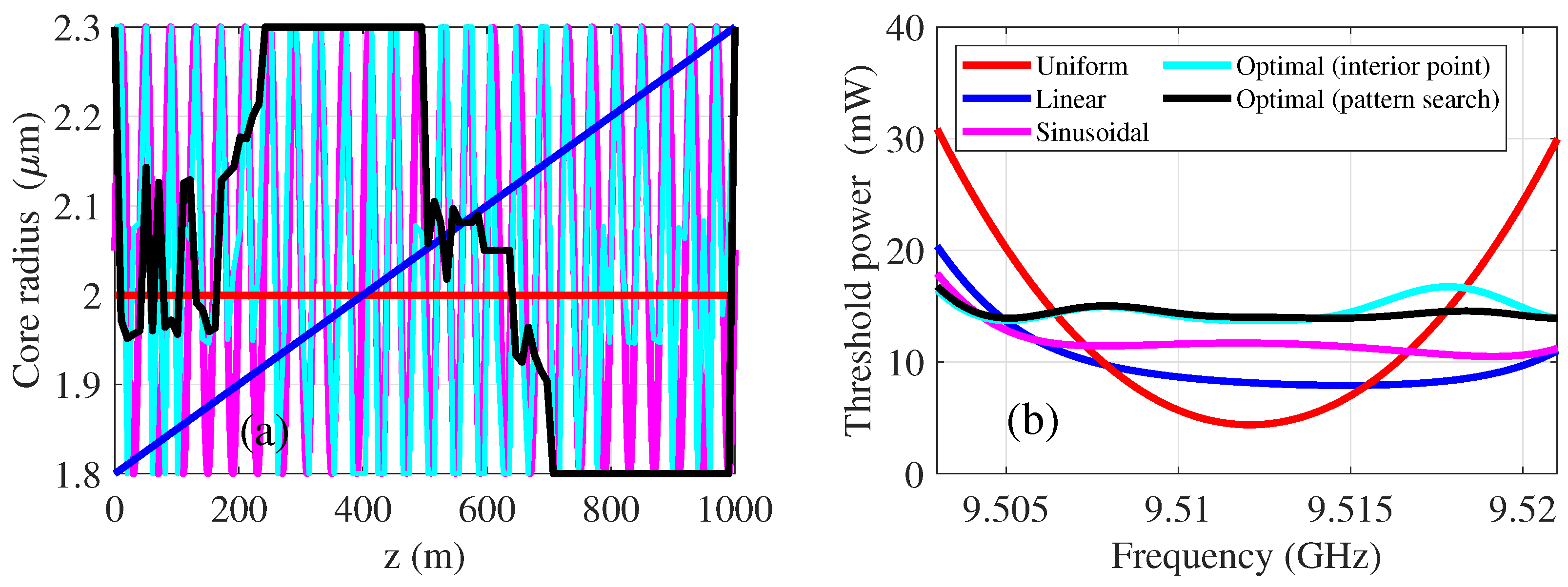
5.3. Numerical Optimization of Longitudinal Fiber Profile for SBS Mitigation

In a uniform optical fiber, the Brillouin Stokes wave naturally builds up throughout the fiber at a specific frequency, which is determined by the fiber’s modal characteristics. However, when we introduce variations in the transverse profile, whether caused by mechanical stress or engineered during the fiber drawing process, a single Brillouin frequency shift is no longer sustainable. As a result, it becomes imperative to scan across a frequency range to determine the Brillouin frequency shift corresponding to the maximum Brillouin gain. The extent of this frequency range depends on the range of variation in the modal characteristics of the fiber incurred due to the transverse change in the fiber profile. Thus for a DOF our objective is to identify the optimal perturbation in the longitudinal fiber profile that maximizes the suppression of SBS. To achieve this, first we compute the modal parameters for various values of the fiber diameter. The core radius $r\left(z\right)$, is discretized along the length of the fiber and the SBS threshold power across a range of Brillouin frequencies is computed numerically using the steady-state approach, with a weak (10⁻¹⁵ W in power) seeded Stokes wave. We employ a non-linear optimization approach using the predictor-corrector interior-point method (within the optimization toolbox in MATLAB [53]) to find a $r\left(z\right)$ that leads to the highest SBS threshold. This method relies on a gradient-based optimization approach and assumes that the objective function is differentiable. Starting from an initial guess, the algorithm computes subsequent points in the direction of gradient descent. Given the unpredictability of the objective function’s variation with respect to a large set of unknown parameters, we also implement both gradient-based and gradient-free pattern search approaches to locate the global optima function for $r\left(z\right)$. The pattern search method, being gradient-free, is suitable for functions that are non-smooth and non-differentiable. This technique calculates the functional value at multiple initial points around an initial guess and proceeds toward the direction of the minimum function value. In our investigation, we observed that the SBS threshold for a sinusoidal variation profile was higher compared to other intuitive designs. Therefore, we adopted a sinusoidal profile as the initial guess for all the optimization algorithms.

In Figure 13a, the radius profiles (optimal and standard) are shown. The corresponding threshold power variation with frequency is plotted in Figure 13b. The SBS threshold power for the optimal profiles are about 14 mW, around 3 times the threshold computed for a constant profile of $r=2 \mathsf{\mu }$m. In fact the sinusoidal profile, which by the way was the optimal profile for the PSA case, also shows an improvement of a factor of two in terms of its SBS threshold power. While the power-frequency response corresponding to both the optimal profiles are similar, the radial variation of the profiles are considerably different, implying that multiple profiles could correspond to a similar threshold characteristics. This also opens new perspectives in terms of investigating the PSA performances of the SBS-optimized radius profiles. Clearly from Figure 13b, we see that the perturbation in the longitudinal radius profiles lead to a flattening effect on the gain spectrum which is typically a Lorentzian distribution for a uniform profile.

The above analysis can also be extended to include the optimization of the profile with respect to the W-ratio of the fiber preform to reduce the acousto-optic overlap. In this investigation we fixed the value of the W-ratio to 2.3. Furthermore, the SBS threshold was evaluated as a function the dispersion oscillation period and the modulation depth which is the ratio of ${\tilde{\beta }}_2$ and ${\overline{\beta }}_2$ [see Figure 14a].

Figure 14a shows that an increase in the modulation depth leads to an elevation of the SBS threshold. This is an expected trend as we reiterate from Equation (5) that the variation in the dispersion profile is only significant when the modulation amplitude is of the same order of magnitude or larger than the average dispersion. On the other hand, the dependence of SBS threshold on the dispersion oscillation wavelength was found to be feeble, albeit present. The inhomogenously separated bands that appear at different modulation wavelengths arise due to the variation of the phase-matching criterion, and is reminiscent of the band structure of modulation instability spectrum in a DOF [11]. As discussed, the Brillouin frequency shift for a uniform fiber represents a singular value that corresponds to the precise phase-matching condition necessary for the Brillouin process to occur. However, in the presence of perturbations or variations along the fiber length, the Brillouin gain can be dispersed over a range of frequencies. This dispersion of the gain implies that the phase-matching condition is satisfied for different frequencies at distinct locations along the length of the fiber. As a result, the Brillouin scattering process is not confined to a single, fixed frequency but is distributed over a spectrum of frequencies. As illustrated in Figure 15, for the system discussed in Figure 14, the periodic variations in the fiber’s properties leads to a distribution of Brillouin frequencies throughout the fiber, effectively demonstrating the impact of modulation on the Brillouin process.

In essence, the act of elevating the SBS threshold brings about a notable consequence—the flattening of the Brillouin gain spectrum. To gauge this phenomenon, we employ a quantitative measure: the 3 dB bandwidth, signifying the range over which the SBS threshold dwindles to precisely half its peak value. As demonstrated in Figure 14b, we graphically depict the relationship between this bandwidth and the corresponding threshold power for different values of modulation depth of three arbitrarily chosen modulation periods: $z_{\mathrm{mod}}=$ 181 m (red filled circles), 281 m (blue filled triangles) and 377 m (magenta filled stars). A clear trend emerges in the plot, showcasing that broader bandwidths align with higher threshold power values. In the context of a uniform fiber, this full Width at half maximum (FWHM) relates to the acoustic line-width, often denoted as ${\Gamma }_B$, which itself is the reciprocal of the phonon lifetime ${\tau }_b$. Remarkably, as shown in the figure, the introduction of dispersion oscillations magnifies this bandwidth manifold, surging from an initial 45 MHz to a substantial 250 MHz. This dramatic expansion in bandwidth equates to a staggering 5 dB augmentation in the threshold power. Thus an astute strategy to mitigate the adverse impacts of SBS in highly non-linear fibers involves selecting a modulation depth that corresponds to a Brillouin frequency shift range surpassing the acoustic linewidth. This approach promises substantial benefits in taming the effects of SBS in speciality optical fibers.

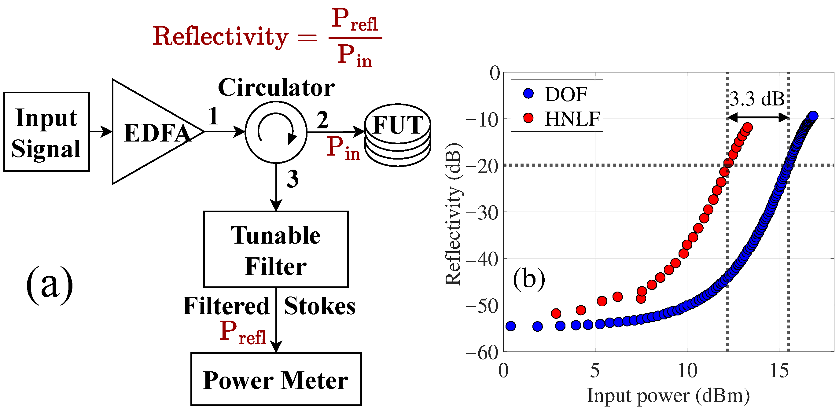
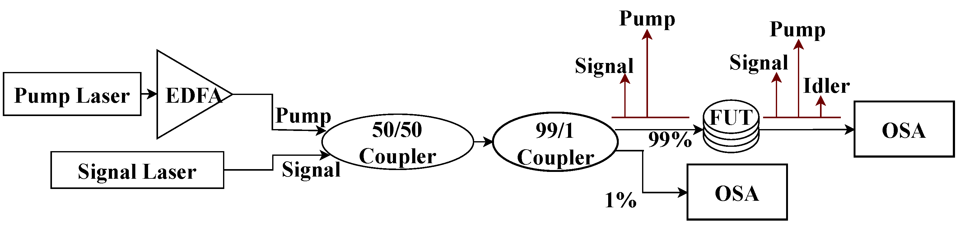
6. Experiments on SBS Mitigation and Parametric Amplification with a DOF

In this section we aim at evaluating the performance of a DOF as a parametric amplifier, in terms of its SBS threshold as well as its conversion efficiency (CE). We compare the DOF’s performance with a standard highly nonlinear fiber (HNLF) with a constant longitudinal dispersion profile.

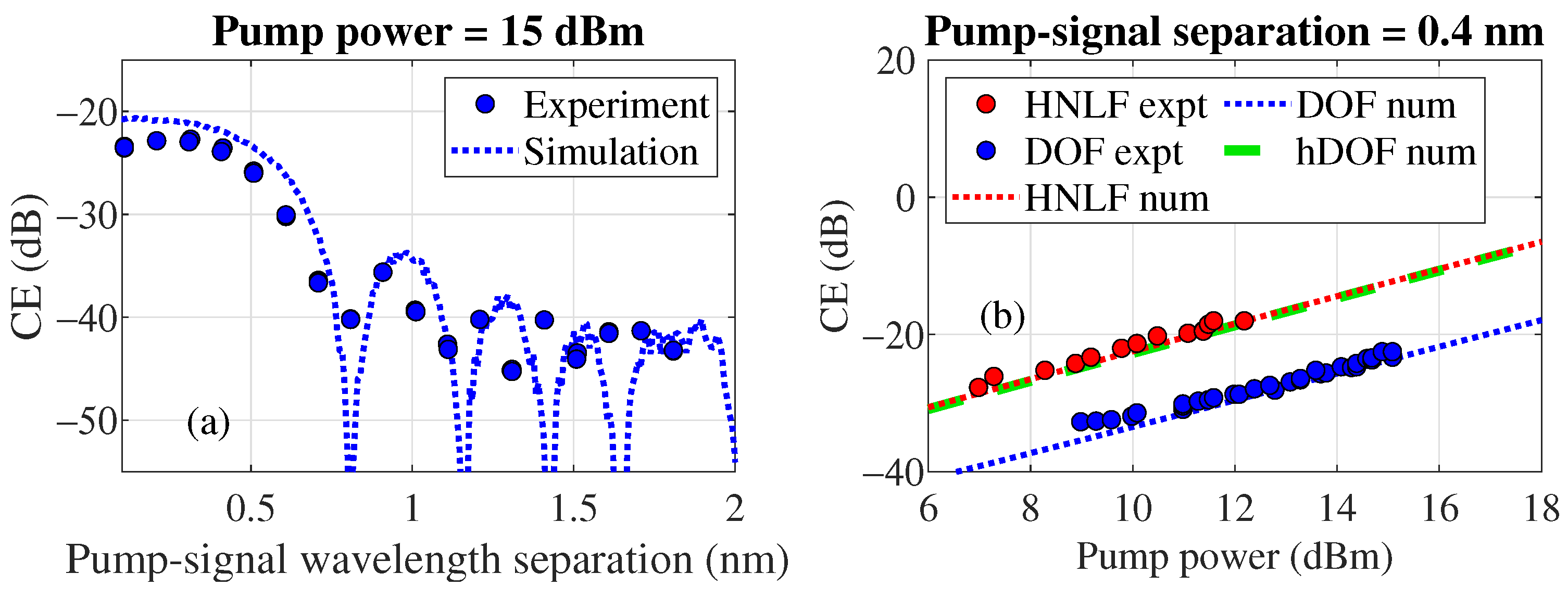
6.1. Comparison of SBS Threshold

In this section, we discuss the experiment to determine the strength of SBS associated with two nonlinear fibers, a DOF and a standard HNLF with constant dispersion. The length of the standard HNLF used is 1 km with a constant dispersion of ${\beta }_2=-0.07$ ps²/km. The available DOF used here is of length 1.25 km and has an oscillating dispersion profile as with a wavelength $z_{\mathrm{mod}}=250$ m and phase ${\phi }_{\mathrm{mod}}=0$ rad. The average dispersion ${\overline{\beta }}_2=12$ ps²/km, dispersion modulation amplitude $\widetilde{{\beta }_2}=2$ ps²/km.

Figure 16a depicts the schematic of the experimental setup that is employed to measure the SBS threshold. First, light from a narrow linewidth laser is passed through an erbium doped fiber amplifier (EDFA) and fed to the fiber under test (FUT) through a circulator. The reflected signal from the FUT obtained at port 3 of the circulator constitutes of pump and the Stokes wave if the input power to FUT is near to or higher than the SBS threshold. The Stokes wave is filtered out from this reflected signal (also containing Rayleigh back-reflections) using a flat-top band pass filter (Yenista, XTM-50) of bandwidth 10 GHz centered at Stokes frequency (10.335 GHz for DOF and 9.634 GHz for HNLF). The power of the filtered Stokes wave for different input power levels is then measured using a powermeter (PM) to obtain the reflectivity as a function of input power, where reflectivity is defined as the ratio of reflected power to input power. The reflectivity for different input power levels for these FUT, indicating a significant difference in the SBS threshold levels are shown in Figure 16. As expected, reflectivity is seen to be increasing with increase in input power in both the fibers. From Figure 16b, the SBS threshold power, which is defined as the input power for which the reflectivity is 1% (−20 dB), is found to be 12.2 dBm for HNLF and 15.5 dBm for DOF. The reflectivity at a particular input power is higher for the HNLF and thus its SBS threshold is correspondingly lower than that of the DOF. In case of the DOF, the coherent build-up of back-scattered waves is prevented through periodic oscillations of dispersion and hence, the threshold is found to be much higher compared to that of the HNLF.

6.2. Comparison of Conversion Efficiency (CE)

The efficacy of using a nonlinear fiber as a parametric amplifier is often quantified by its conversion efficiency (CE) of converting an input signal to a conjugate idler through four wave mixing (FWM) involving the pump. Thus CE is basically the ratio of the output idler power to the input signal power. To find the CE of the DOF used, we perform an experiment schematically represented in Figure 17. A degenerate pump and a signal are launched into the nonlinear fiber (HNLF or DOF) and the power of the input signal as well as the output idler are recorded for different pump powers and pump-signal detuning, using an optical spectrum analyzer (OSA).

We compared the experimental results, with a numerical NLSE model introduced in Section 4.2. The fiber parameters for the DOF and the HNLF are same as in the previous subsection. The nonlinear coefficient $\gamma$ for the DOF and HNLF used are, 3.5 and 11.1 (W km)⁻¹.

The validation of the NLSE based simulation model is achieved through comparing the CE as a function of pump-signal wavelength separation obtained from the experiment as shown in Figure 18a. On the other hand, in Figure 18b, we investigate the CE of the DOF (blue) and the HNLF (red) as a function of the input pump power, both through the simulation (dotted lines) and the experiment (filled circles). The input signal power is 7 dBm. Needless to say, the experimental data satisfactorily conform to the numerically predicted trend. From Figure 18b, we find that the DOF, similar to a standard HNLF, show a linear growth of CE with respect to the pump power (in a log-log scale). The 10 dB difference between the DOF and the HNLF in Figure 18b arise due to the combined effect of their unequal nonlinear coefficients, average dispersion values and lengths. To confirm this hypothesis, we simulated the same curve for a hypothetical DOF (hDOF) with the same length, $\gamma$ and ${\overline{\beta }}_2$ as the HNLF (see green dashed curve in Figure 18b). Indeed, we find the CE curve of the hDOF to coincide with that of the HNLF, confirming the CE is almost unaffected due to the dispersion oscillation.

7. Discussion

As discussed previously, in this article we study the employment of a DOF as a PSA from two different vantage points in the case of the single and dual pump configurations. Therefore in this section we outline the implications of our performed investigations separately for these two configurations.

7.1. Single Pump PSA with DOF

In the single pump PSA case, the effect of longitudinal dispersion variation leads to the emergence of high-order PSA gain sidebands (>20 dBm signal gain and a bandwidth of 22 GHz for $q=1$) at large pump-signal detunings, of the order of a few Terahertz. The ability to achieve PSA functionality at these large detunings in a single pump configuration using just longitudinal dispersion variation is already an interesting aspect of the investigated system. Furthermore, the obtained numerical results show us the presence of an anti-gain dip within the high-order gain band. The spectral position of this dip can be controlled either by varying the input pump phase $\theta$, or by changing the phase of the dispersion modulation ${\phi }_{\mathrm{mod}}$, allowing the system to behave as a tunable notch filter within the gain band. Furthermore, to flatten and broaden the gain band, the dispersion profile was generated with multiple optimized dispersion oscillation frequencies. This led to the flattening of the gain band and broadened the spectrum almost two folds, however at a cost of a reduced signal gain. Although such a multi-frequency profile is highly interesting in terms of its bandwidth and tunability, fabrication of such a fiber will require precise control over the drawn fiber’s core radius, and might pose a technological hurdle in practice. Nevertheless, these results are highly encouraging for the development of modern all optical signal processing techniques. For example, in all optical network as in [54], add/drop operation of modulated optical signals can be achieved through a real time control over the pump phase that can precisely position an anti-gain dip at the frequency of a channel to be dropped in a WDM signal. We should also remind, that the longitudinal sinusoidal dispersion variation of the DOF should provide an additional advantage in launching larger pump powers into the system as already discussed in Section 5 and Section 6.

7.2. Dual Pump PSA with DOF

For the case of a dual pump PSA, our focus was primarily fixated on improving the signal gain of the system. Using analytical and numerical approaches, we argued that a sinusoidally varying profile can provide the largest gain, while profiles with multiple frequencies or a uniform profile tend to flatten out the gain spectrum. Thus we considered a dual pump PSA system with a sinusoidal dispersion profile and numerically evaluated the maximum signal gain by scanning the dispersion oscillation amplitude ${\tilde{\beta }}_2$ and the average second order dispersion ${\overline{\beta }}_2$. The effect of dispersion oscillation amplitude was found to be pronounced, only when ${\overline{\beta }}_2$ is close to 0. This is because only then $\widetilde{{\beta }_2}$ becomes comparable to ${\overline{\beta }}_2$ and the dispersion oscillation effects are not averaged out over the fiber length. For the case of ${\overline{\beta }}_2$ is close to 0, depending on the choice of $\widetilde{{\beta }_2}$, a large range of gain, gain flatness and gain bandwidth is possible.

On the other hand, with respect to the SBS performance, although the sinusoidal profile had a higher SBS threshold than a uniform or linear profile, it was slightly outperformed by other profiles obtained through optimization techniques. Therefore, for highly specific applications with targeted gain, gain bandwidth and gain flatness requirements, an advanced nonlinear optimization approach is required to optimize the SBS as well as the PSA performance simultaneously. However, our investigation outright suggests the advantage of using a DOF as a dual pump PSA over a standard HNLF in terms of achieving a larger PSA gain, considering the same nonlinearity in both. To validate these claims, we performed two experiments, one for the SBS and the other for the PSA to compare the performance of a DOF with that of a standard HNLF. In the SBS experiment, the DOF exhibited about 3 dB improvement of the SBS threshold over the HNLF, as expected. However, the conversion efficiency (CE) of the DOF was found to be about 10 dB lower in the case of the DOF compared to the HNLF. But the CE result should be treated with a caveat, since the DOF and the HNLF used in the experiment had different lengths, dispersion values and nonlinear coefficients. In fact, a numerically calculated CE of a DOF with the same nonlinear parameters of the HNLF shows that a DOF and a HNLF can provide the same CE, which is a crucial quantifier for the PSA gain of the system. These results convincingly prove that a DOF can outperform a standard HNLF in terms of its gain performance in a dual pump PSA system.

Another important technical question about the PSA functionality of a DOF is that how to fabricate a DOF with a large nonlinear coefficient? This question might be addressed in a few different ways. For example, the nonlinear coefficient of a nonlinear fiber can be increased by reducing further the average core radius of the DOF. However that might lead to a change in the dispersion properties of the fiber and hence additional nonlinear optimization may be required to optimize the PSA performance. Also, changing the doping concentration in the preform might be a resource to ramp up the nonlinear coefficient of the fiber. Additionally, modifying the fiber preform profile might be another approach in this regard, that can not only provide a handle over controlling the fiber nonlinearity, but also the acousto-optic overlap for SBS mitigation [55].

8. Conclusions

To conclude, in this article we provided a comprehensive study on designing a fiber phase sensitive amplifier with a dispersion tailored fiber. This study suggests that fibers with a sinusoidally oscillating dispersion profile is a very strong candidate for the development of PSAs with a large gain, owing to the ability to launch high pump powers due to an elevated SBS threshold. While dual pump PSAs provide a large gain advantage, single pump PSAs can be tailored to develop amplifiers and filters at large pump-signal detunings. It was shown that the phase-sensitive amplification attribute can be realized in high-order modulation instability sidebands of a single pump PSA. Further, we discovered the system’s ability to act as a high extinction-ratio filter at frequencies that are tunable with respect to the phase of the input pump, or the phase of dispersion oscillation. We also propose the use of DOFs for generation of a comb of multiple spectral sidebands with phase-sensitive gain, that can find numerous applications.

We also studied the SBS mitigation properties of dispersion varying profiles numerically and optimal profiles were proposed targeted at acquiring large SBS thresholds. The ability of a DOF to be used in a large-gain PSA were also confirmed experimentally both in terms of its SBS performance as well as a parametric amplifier. These investigations definitely open new possibilities to further optimize the dispersion profile of a DOF and build PSAs that can outcompete standard HNLFs with a superior performance.

References

1. Caves, C.M. Quantum limits on noise in linear amplifiers. Phys. Rev. D 1982, 26, 1817. [Google Scholar] [CrossRef]
2. Lim, O.K.; Grigoryan, V.; Shin, M.; Kumar, P. Ultra-low-noise inline fiber-optic phase-sensitive amplifier for analog optical signals. In Proceedings of the Optical Fiber Communication Conference, San Diego, CA, USA, 24–28 February 2008; p. OML3. [Google Scholar]
3. Tong, Z.; Lundström, C.; Andrekson, P.A.; Karlsson, M.; Bogris, A. Ultralow noise, broadband phase-sensitive optical amplifiers, and their applications. IEEE J. Sel. Top. Quantum Electron. 2011, 18, 1016–1032. [Google Scholar] [CrossRef]
4. Malik, R.; Kumpera, A.; Lorences-Riesgo, A.; Andrekson, P.; Karlsson, M. Frequency-resolved noise figure measurements of phase (in) sensitive fiber optical parametric amplifiers. Opt. Express 2014, 22, 27821–27832. [Google Scholar] [CrossRef]
5. Andrekson, P.A.; Karlsson, M. Fiber-based phase-sensitive optical amplifiers and their applications. Adv. Opt. Photonics 2020, 12, 367–428. [Google Scholar] [CrossRef]
6. Tang, R.; Devgan, P.S.; Grigoryan, V.S.; Kumar, P.; Vasilyev, M. In-line phase-sensitive amplification of multi-channel CW signals based on frequency nondegenerate four-wave-mixing in fiber. Opt. Express 2008, 16, 9046–9053. [Google Scholar] [CrossRef]
7. Sodré, A.C.; Cañas-Estrada, N.; Noque, D.F.; Borges, R.M.; Melo, S.A.; González, N.G.; Oliveira, J.C. Photonic-assisted microwave amplification using four-wave mixing. IET Optoelectron. 2016, 10, 163–168. [Google Scholar] [CrossRef]
8. Zhao, P.; Kakarla, R.; Karlsson, M.; Andrekson, P.A. Enhanced analog-optical link performance with noiseless phase-sensitive fiber optical parametric amplifiers. Opt. Express 2020, 28, 23534–23544. [Google Scholar] [CrossRef]
9. Kakarla, R.; Schröder, J.; Andrekson, P.A. One photon-per-bit receiver using near-noiseless phase-sensitive amplification. Light. Sci. Appl. 2020, 9, 153. [Google Scholar] [CrossRef]
10. Fedorov, M. Entanglement of multiphoton states in polarization and quadrature variables. Laser Phys. 2019, 29, 124006. [Google Scholar] [CrossRef]
11. Droques, M.; Kudlinski, A.; Bouwmans, G.; Martinelli, G.; Mussot, A. Experimental demonstration of modulation instability in an optical fiber with a periodic dispersion landscape. Opt. Lett. 2012, 37, 4832–4834. [Google Scholar] [CrossRef]
12. Finot, C.; Fatome, J.; Sysoliatin, A.; Kosolapov, A.; Wabnitz, S. Competing four-wave mixing processes in dispersion oscillating telecom fiber. Opt. Lett. 2013, 38, 5361–5364. [Google Scholar] [CrossRef]
13. Feng, F.; Fatome, J.; Sysoliatin, A.; Chembo, Y.; Wabnitz, S.; Finot, C. Wavelength conversion and temporal compression of pulse train using dispersion oscillating fibre. Electron. Lett. 2014, 50, 768–770. [Google Scholar] [CrossRef]
14. Mussot, A.; Conforti, M.; Trillo, S.; Copie, F.; Kudlinski, A. Modulation instability in dispersion oscillating fibers. Adv. Opt. Photonics 2018, 10, 1–42. [Google Scholar] [CrossRef]
15. Mazhirina, Y.A.; Mel’nikov, L.A.; Sysoliatin, A.; Konyukhov, A.I.; Gochelashvili, K.S.; Venkitesh, D.; Sarkar, S. Parametric amplification in optical fibre with longitudinally varying dispersion. Quantum Electron. 2021, 51, 692. [Google Scholar] [CrossRef]
16. Chatterjee, D.; Bouasria, Y.; Xie, W.; Labidi, T.; Goldfarb, F.; Fsaifes, I.; Bretenaker, F. Investigation of analog signal distortion introduced by a fiber phase sensitive amplifier. J. Opt. Soc. Am. B 2020, 37, 2405–2415. [Google Scholar] [CrossRef]
17. Smith, N.; Doran, N. Modulational instabilities in fibers with periodic dispersion management. Opt. Lett. 1996, 21, 570–572. [Google Scholar] [CrossRef]
18. Fourcade-Dutin, C.; Bassery, Q.; Bigourd, D.; Bendahmane, A.; Kudlinski, A.; Douay, M.; Mussot, A. 12 THz flat gain fiber optical parametric amplifiers with dispersion varying fibers. Opt. Express 2015, 23, 10103–10110. [Google Scholar] [CrossRef]
19. Da Ros, F.; Dalgaard, K.; Lei, L.; Xu, J.; Peucheret, C. QPSK-to-2× BPSK wavelength and modulation format conversion through phase-sensitive four-wave mixing in a highly nonlinear optical fiber. Opt. Express 2013, 21, 28743–28750. [Google Scholar] [CrossRef]
20. Xie, W.; Fsaifes, I.; Bretenaker, F. Optimization of a degenerate dual-pump phase-sensitive optical parametric amplifier for all-optical regenerative functionality. Opt. Express 2017, 25, 12552–12565. [Google Scholar] [CrossRef]
21. Baillot, M.; Gay, M.; Peucheret, C.; Michel, J.; Chartier, T. Phase quadrature discrimination based on three-pump four-wave mixing in nonlinear optical fibers. Opt. Express 2016, 24, 26930–26941. [Google Scholar] [CrossRef]
22. Chatterjee, D.; Bouasria, Y.; Goldfarb, F.; Hassouni, Y.; Bretenaker, F. Optimization of the conversion efficiency and evaluation of the noise figure of an optical frequency converter based on a dual-pump fiber phase sensitive amplifier. Opt. Express 2022, 30, 45676–45693. [Google Scholar] [CrossRef]
23. Marhic, M.E. Fiber Optical Parametric Amplifiers, Oscillators and Related Devices; Cambridge University Press: Cambridge, MA, USA, 2008. [Google Scholar]
24. Konyukhov, A.; Mavrin, P.; Suchita; Sobhanan, A.; Venkitesh, D.; Gochelashvili, K.; Sysoliatin, A. Phase-sensitive amplification in dispersion oscillating fibers. Laser Phys. 2021, 31, 085402. [Google Scholar] [CrossRef]
25. Yoshizawa, N.; Imai, T. Stimulated Brillouin scattering suppression by means of applying strain distribution to fiber with cabling. J. Light. Technol. 1993, 11, 1518–1522. [Google Scholar] [CrossRef]
26. Rothenberg, J.E.; Thielen, P.A.; Wickham, M.; Asman, C.P. Suppression of stimulated Brillouin scattering in single-frequency multi-kilowatt fiber amplifiers. In Proceedings of the Fiber Lasers V: Technology, Systems, and Applications, San Jose, CA, USA, 21–24 January 2008; Volume 6873, pp. 104–110. [Google Scholar]
27. Imai, Y.; Shimada, N. Dependence of stimulated Brillouin scattering on temperature distribution in polarization-maintaining fibers. IEEE Photonics Technol. Lett. 1993, 5, 1335–1337. [Google Scholar] [CrossRef]
28. Hansryd, J.; Dross, F.; Westlund, M.; Andrekson, P.; Knudsen, S. Increase of the SBS threshold in a short highly nonlinear fiber by applying a temperature distribution. J. Light. Technol. 2001, 19, 1691. [Google Scholar] [CrossRef]
29. Dianov, E.M.; Zel’dovich, B.Y.; Karasik, A.Y.; Pilipetskiĭ, A.N. Feasibility of suppression of steady-state and transient stimulated Brillouin scattering. Sov. J. Quantum Electron. 1989, 19, 1051. [Google Scholar] [CrossRef]
30. Kikuchi, K.; Lorattanasane, C. Design of highly efficient four-wave mixing devices using optical fibers. IEEE Photonics Technol. Lett. 1994, 6, 992–994. [Google Scholar] [CrossRef]
31. Zeringue, C.; Dajani, I.; Naderi, S.; Moore, G.T.; Robin, C. A theoretical study of transient stimulated Brillouin scattering in optical fibers seeded with phase-modulated light. Opt. Express 2012, 20, 21196–21213. [Google Scholar] [CrossRef]
32. Supradeepa, V. Stimulated Brillouin scattering thresholds in optical fibers for lasers linewidth broadened with noise. Opt. Express 2013, 21, 4677–4687. [Google Scholar] [CrossRef]
33. Anderson, B.; Flores, A.; Holten, R.; Dajani, I. Comparison of phase modulation schemes for coherently combined fiber amplifiers. Opt. Express 2015, 23, 27046–27060. [Google Scholar] [CrossRef]
34. Gordienko, V.; Szabó, Á.; Stephens, M.; Vassiliev, V.; Gaur, C.; Doran, N. Limits of broadband fiber optic parametric devices due to stimulated Brillouin scattering. Opt. Fiber Technol. 2021, 66, 102646. [Google Scholar] [CrossRef]
35. Agrawal, G. Nonlinear Fiber Optics, 5th ed.; Elsevier: Amsterdam, The Netherlands, 2013. [Google Scholar]
36. Mussot, A.; Durecu-Legrand, A.; Lantz, E.; Simonneau, C.; Bayart, D.; Maillotte, H.; Sylvestre, T. Impact of pump phase modulation on the gain of fiber optical parametric amplifier. IEEE Photonics Technol. Lett. 2004, 16, 1289–1291. [Google Scholar] [CrossRef]
37. Wong, K.K.; Marhic, M.E.; Kazovsky, L.G. Phase-conjugate pump dithering for high-quality idler generation in a fiber optical parametric amplifier. IEEE Photonics Technol. Lett. 2003, 15, 33–35. [Google Scholar] [CrossRef]
38. Shiraki, K.; Ohashi, M.; Tateda, M. Suppression of stimulated Brillouin scattering in a fibre by changing the core radius. Electron. Lett. 1995, 31, 668–669. [Google Scholar] [CrossRef]
39. Lundin, R. Dispersion flattening in a W fiber. Appl. Opt. 1994, 33, 1011–1014. [Google Scholar] [CrossRef]
40. Snyder, A.; Love, J. Optical Waveguide Theory; Chapman and Hall: London, UK, 1983; Chapter 19. [Google Scholar]
41. Boyd, R.W. Nonlinear Optics; Academic Press: Cambridge, MA, USA, 2020. [Google Scholar]
42. Inoue, K. Influence of multiple four-wave-mixing processes on quantum noise of dual-pump phase-sensitive amplification in a fiber. JOSA B 2019, 36, 1436–1446. [Google Scholar] [CrossRef]
43. Chatterjee, D.; Bouasria, Y.; Goldfarb, F.; Bretenaker, F. Analytical seven-wave model for wave propagation in a degenerate dual-pump fiber phase sensitive amplifier. JOSA B 2021, 38, 1112–1124. [Google Scholar] [CrossRef]
44. Hansryd, J.; Andrekson, P.A.; Westlund, M.; Li, J.; Hedekvist, P.O. Fiber-based optical parametric amplifiers and their applications. IEEE J. Sel. Top. Quantum Electron. 2002, 8, 506–520. [Google Scholar] [CrossRef]
45. Ferrini, G.; Fsaifes, I.; Labidi, T.; Goldfarb, F.; Treps, N.; Bretenaker, F. Symplectic approach to the amplification process in a nonlinear fiber: Role of signal-idler correlations and application to loss management. J. Opt. Soc. Am. B 2014, 31, 1627–1641. [Google Scholar] [CrossRef]
46. Xie, W.; Fsaifes, I.; Labidi, T.; Bretenaker, F. Investigation of degenerate dual-pump phase sensitive amplifier using multi-wave model. Opt. Express 2015, 23, 31896–31907. [Google Scholar] [CrossRef]
47. Wong, K.K.; Marhic, M.E.; Uesaka, K.; Kazovsky, L.G. Polarization-independent two-pump fiber optical parametric amplifier. IEEE Photonics Technol. Lett. 2002, 14, 911–913. [Google Scholar] [CrossRef]
48. Hu, H.; Jopson, R.; Gnauck, A.; Dinu, M.; Chandrasekhar, S.; Xie, C.; Randel, S. Parametric amplification, wavelength conversion, and phase conjugation of a 2.048-Tbit/s WDM PDM 16-QAM signal. J. Light. Technol. 2015, 33, 1286–1291. [Google Scholar] [CrossRef]
49. Chatterjee, D.; Konyukhov, A.; Sysoliatin, A.; Venkitesh, D. Phase-Sensitive Amplification in a Dispersion Oscillating Fiber with Two Pumps. In Proceedings of the Asia Communications and Photonics Conference, Shanghai, China, 24–27 October 2021; p. W2A.3. [Google Scholar]
50. Stolen, R.; Bjorkholm, J. Parametric amplification and frequency conversion in optical fibers. IEEE J. Quantum Electron. 1982, 18, 1062–1072. [Google Scholar] [CrossRef]
51. Smith, R.G. Optical power handling capacity of low loss optical fibers as determined by stimulated Raman and Brillouin scattering. Appl. Opt. 1972, 11, 2489–2494. [Google Scholar] [CrossRef]
52. Haneef, S.M.; Prashanth, P.; Venkitesh, D.; Srinivasan, B. Modeling Stimulated Brillouin Scattering in LEAF Using Finite Difference Method. In Proceedings of the International Conference on Fibre Optics and Photonics, Virtual, 13–16 December 2014; p. S5A.39. [Google Scholar]
53. MATLAB, Version R2021b; The MathWorks Inc.: Natick, MA, USA, 2021.
54. Brackett, C.A.; Acampora, A.S.; Sweitzer, J.; Tangonan, G.; Smith, M.T.; Lennon, W.; Wang, K.C.; Hobbs, R.H. A scalable multiwavelength multihop optical network: A proposal for research on all-optical networks. J. Light. Technol. 1993, 11, 736–753. [Google Scholar] [CrossRef]
55. Dong, L. Limits of stimulated Brillouin scattering suppression in optical fibers with transverse acoustic waveguide designs. J. Light. Technol. 2010, 28, 3156–3161. [Google Scholar]
Figure 1. An illustration of the sinusoidal longitudinal variation of the core, trench and cladding radius of a W-type fiber. Input configurations of a dual-pump and single pump PSA are shown in left insets. A qualitative refractive index ( R I ) profile in arbitrary units along the transverse direction (y-direction) is shown in solid red line in th right inset. a and b are the core and trench diameters respectively (not to scale).
Photonics 11 00003 g001
Figure 2. False color plots of (a) β 2 , (b) β 3 and (c) β 4 as a function of the core radius and W-ratio = b / a calculated from the mode solver.
Photonics 11 00003 g002
Figure 3. An illustration of the signal, pump and idler for a single pump PSA configuration. Ω p s is the pump-signal angular frequency separation. 0, 1 and −1 refer to the indices of the waves. (not to scale).
Photonics 11 00003 g003
Figure 4. The parametric gain in regimes of the anomalous and normal average dispersion. (a) β ¯ 2 = 2.16   ps 2 km 1 , β ˜ 2 = 3.1   ps 2 km 1 , β ¯ 4 = 3.4 × 10 4   ps 4 km 1 , and β ˜ 4 = 0.19 × 10 4   ps 4 km 1 . (b,c) β ¯ 2 = 2.16   ps 2 km 1 , β ˜ 2 = 2.98   ps 2 km 1 , β ¯ 4 = 3.77 × 10 4   ps 4 km 1 , and β ˜ 4 = 0.32 × 10 4   ps 4 km 1 . Pump-signal separation is ( λ p λ s ) , where λ p is 1550 nm. Fiber length L = 1.4   km , modulation period z mod = 40 m, pump power P 0 = 0.5 W, φ mod = 0 , θ = 0 . Other fiber parameters are provided in text.
Photonics 11 00003 g004
Figure 5. Plot of gain of the signal as a function of the pump-signal frequency separation for different values of the initial phase θ in radians. (a,b) φ mod = 0 rad; (c,d) φ mod = 1.2 rad. q = 1 in left column and q = 2 in right column. Other fiber parameters are the same as in Figure 4b,c.
Photonics 11 00003 g005
Figure 6. (a) Fiber dispersion parameters as a function of the propagation length. (b,c) Plot of gain of the signal as a function of the pump-signal frequency separation for different values of the initial phase of the pump wave θ . q = 1 in (b) and q = 2 in (c). Fiber length L = 1.4   km , γ = 9.44 (W km)−1. Other fiber parameters are provided in text.
Photonics 11 00003 g006
Figure 7. Phase-spectral distribution of the gain G S for q = 1 (a) and q = 2 (b). Parameters are same as in Figure 6.
Photonics 11 00003 g007
Figure 8. An illustration of the degenerate signal and the two pumps considered in a three-wave model. Notations are same as Figure 3.
Photonics 11 00003 g008
Figure 9. False colour plots of maximum PSA signal gain (ac,gi) and gain extinction ratio (df) as a function of the pump-signal frequency separation Ω p s 2 π and amplitude of dispersion oscillation β 2 ˜ (denoted as β 2 , a m ). Top and middle row correspond to numerically calculated results, while the bottom row is from the analytical 3-wave model. Three different average second order dispersion β ¯ 2 (denoted as β 2 , a v ) values are considered: (a,d,g) −5 ps2/km, (b,e,h) 0 ps2/km and (c,f,i) 5 ps2/km. L = 1000 m, γ = 4 (W km)−1, P = 22 dBm.
Photonics 11 00003 g009
Figure 10. Same figure as Figure 9, except γ = 10 (W km)−1.
Photonics 11 00003 g010
Figure 11. False color plot of β 2 showing a region where β 2 is within −10 ps2/km and 10 ps2/km. Horizontal dashed line indicate W-ratio b / a = 3 and vertical dashed lines indicate values of β 2 = 5 , 0 , 5 ps2/km.
Photonics 11 00003 g011
Figure 12. (a) Numerically computed maximum PSA gain vs. pump-signal frequency separation for four different profiles. A random profile (in magenta), a profile with single dispersion oscillation wavelength z m 1 = 97 m (in red), double dispersion oscillation wavelength, z m 1 = 97 m and z m 2 = 111 m (in blue) and triple dispersion oscillation wavelength, z m 1 = 97 m, z m 2 = 111 m and z m 3 = 122 m (in green). (b) Variation of outer diameter as a function of length for the same profiles. L = 500 m, γ = 10 (W km)−1, β ¯ 2 = 1 ps2/km and P = 22 dBm.
Photonics 11 00003 g012
Figure 13. (a) Variation of core radius along the length of the fiber for different profiles. (b) Numerically computed SBS threshold power as a function of the seed frequency for different profiles. Uniform profile in red, linear profile in blue, sinusoidal profile in magenta, computed optimal profiles through interior point method in cyan and through pattern search method in black. Other parameters are provided in the text.
Photonics 11 00003 g013
Figure 14. (a) False color plot of SBS threshold power vs. dispersion oscillation wavelength z mod vs. modulation depth β ˜ 2 / β ¯ 2 . (b) SBS threshold power vs. 3 dB bandwidth of reflected Stokes wave for different modulation depths [along the grey dashed lines in (a)], considering different dispersion modulation wavelength: z mod = 181 m (red filled circles), 281 m (blue filled triangles) and 377 m (magenta filled stars). These values of z mod are demarcated with dashed lines in (a). Parameters of the DOF are provided in the text.
Photonics 11 00003 g014
Figure 15. Brillouin frequency shift vs. length of the fiber considering different dispersion modulation wavelength: z mod = 181 m (red), 281 m (blue) and 377 m (magenta). Parameters of the DOF are provided in the text.
Photonics 11 00003 g015
Figure 16. (a) Scheme of the experimental setup for measuring the back reflected power from a nonlinear fiber due to SBS. EDFA: Erbium doped fiber amplifier; FUT: Fiber under test; PM: Powermeter. (b) Experimental data of reflectivity vs. input pump power for a standard HNLF (blue filled circles) and a DOF (red filled circles). Intersection of the dashed lines denote the location of 1% reflectivity of input power due to SBS. Fiber parameters are provided in the text.
Photonics 11 00003 g016
Figure 17. Experimental scheme for the measurement of CE of a nonlinear fiber (HNLF or DOF). OSA: Optical spectrum analyzer; FUT: Fiber under test; EDFA: Erbium doped fiber amplifier. The input and output spectra of the FUT illustrated with brown arrows.
Photonics 11 00003 g017
Figure 18. Plot of conversion efficiency as a function of (a) the pump-signal wavelength separation and (b) input pump power, both from the experiment (filled circles) and the NLSE simulation (dotted and dashed lines). The data corresponding to the DOF is shown in blue while that of the standard HNLF is in red. The green dashed curve correspond to a hypothetical DOF (hDOF) with the same length, γ and β ¯ 2 as the HNLF. Other parameters are provided in the text.
Photonics 11 00003 g018