Three-Airy Beams, Their Propagation in the Fresnel Zone, the Autofocusing Plane Location, as Well as Generalizing Beams


1
Lebedev Physical Institute, Samara 443011, Russia
2
Image Processing Systems Institute, NRC “Kurchatov Institute”, 151 Molodogvardeyskaya St., Samara 443001, Russia
3
Samara National Research University, 34 Moskovskoe Shosse, Samara 443086, Russia
*
Author to whom correspondence should be addressed.
Photonics 2024, 11(4), 312; https://doi.org/10.3390/photonics11040312
Submission received: 2 March 2024
/
Revised: 25 March 2024
/
Accepted: 26 March 2024
/
Published: 28 March 2024
(This article belongs to the Special Issue Laser Beam Propagation and Control)
Abstract
:A family of 2D light fields consisting of the product of three Airy functions with linear arguments has been studied theoretically and experimentally. These fields, called three-Airy beams, feature a parameter shift and have a cubic phase and a super-Gaussian circular intensity in the far zone. Transformations of three-Airy beams in the Fresnel zone have been studied using theoretical, numerical, and experimental means. It has been shown that the autofocusing plane of a three-Airy beam is similar to the square root of the shift parameter. We also introduce generalized three-Airy beams containing nine free parameters, and obtain their Fourier transform in a closed form.
1. Introduction
Light fields based on the Airy function usage are intensively studied objects in modern optics. As a solution of the 1D paraxial equation, the Airy function first appeared in 1979, when the non-diffracting Airy beams of infinite energy were found [1]. However, a boom in optical research related to the Airy function began in 2007, when it was noted that a linear exponential factor allows the construction of paraxial Airy beams of finite energy [2]. In general, Airy beams depend on some real parameters and are functionally stable solutions of the paraxial equation. Despite the lack of structural stability, under certain restrictions, there is a propagation zone in which the intensity of Airy beams varies very weakly. In addition, the parabolic shape of the propagation trajectory of Airy beams provides new opportunities for the practical application of such beams since traditional Gaussian beams are characterized by rectilinear propagation.
This discovery was followed by studies and publications that looked at various aspects related to Airy beams. Among the theoretical works, the following results should be noted: the transformation of Airy–Gaussian beams in first-order optical systems [3], the Poynting vector and orbital angular momentum of Airy beams [4], the nonparaxial study of Airy beams [5,6], truncated Airy beams [7,8], the comparison of Airy beams and Hermite–Gaussian modes under astigmatic transformation [7], vortex Airy beams [7,9] and others [10,11,12,13,14]. Among the experimental works, we mention papers related to the study of the propagation of Airy beams in various media [15,16,17], as well as the use of Airy beams for problems related to microparticles [18] (see also the references therein).
As a rule, either 1D Airy beams or their 2D analogs, obtained by multiplying two 1D beams whose arguments are orthogonal Cartesian coordinates in the plane, were considered. Airy beams of more complex shape (for example, circular Airy beams) have been investigated only numerically and experimentally since theoretical study requires the discovery of quite nontrivial integrals in a closed form. However, the theory of integral transformations of Airy functions is not yet sufficiently developed to cope with such challenges.
One of the nontrivial examples when theoretical research turned out to be possible is a family of three-Airy beams [19]. In 2010, these beams were introduced as the product of three 1D Airy patterns, which are shifted from the origin to the vertices of an equilateral triangle and rotated so that the resulting field is invariant under rotation by :
where
is the Airy function definition, is a 2D vector, and c is a shift parameter.
The shift parameter determines the shape of the three-Airy beams and their behavior when propagating in the Fresnel zone. As it turned out, the Fourier transform of these beams has a cubic phase and a circular super-Gaussian intensity [19]:
Here, is a 2D vector, b is a scaling factor,
is 2D Fourier transform, and is the standard scalar product of 2D vectors. As is seen in (3), only the Airy factor depends on the shift parameter. A simple proof of the relation (3) is presented in Appendix A.
The most interesting cases are when, at the central point, , the Airy function reaches a maximum (i.e., ) or goes to zero (i.e., ). Here and are zeros of the functions and , respectively. All of them are real and located on the negative semi-axis. Asymptotic expansions are known for both families of zeros [20],
Even for small n, the initial terms of these expansions give a very good approximation to the exact values of the zeros. For example,
where the first number is the exact value of zero, and the second is due to Equation (5).
In subsequent years, three-Airy beams were constructed and studied in various ways. Torre in [21] found their intensity moments of second order. In [22], the three-Airy beam for the case was implemented on the basis of the Fourier transform method. Its propagation in free space and a nonlinear medium (SBN crystal) was studied experimentally. In [23], Desyatnikov et al. also used the Fourier transform method, but the initial field was formed by the holographic method. In that article, two beams with parameters and were investigated, and autofocusing of three-Airy beams was discussed. In addition, Desyatnikov considered the propelling behavior of such beams when an optical singularity is embedded, as well as the prospects for their use for transporting particles. In [24], vortex three-Airy beams with different topological charges have been investigated.
In this work, we continue to study three-Airy beams by theoretical and numerical means, as well as in optical experiments. In Section 2, we discuss the ways to evaluate the Fresnel transform of these beams. Here, the experimental implementation of three-Airy beams is also considered. In Section 3, we investigate the autofocusing behavior of these beams. In Section 4, we generalize the relation (3) and provide some corollaries concerning the beams of finite and infinite energy. In Conclusion, we discuss possible applications of the results obtained.
We consider the study of three-Airy beams at various values of the shift parameter, the characteristics of their propagation in the Fresnel zone, and the determination of the autofocusing plane depending on the shift parameter as a necessary basis for the subsequent transition to the study of multiple beams of Pearcey, swallowtail, and other diffraction catastrophes, whose non-Gaussian nature also leads to the appearance of an autofocusing plane when propagating in the Fresnel zone.
2. Three-Airy Beams in the Fresnel Diffraction Zone
2.1. Theory
If a coherent light field of a wavelength is specified by its complex amplitude in the initial plane , then the field propagation in free space is described in the paraxial approximation by the equation , where . If vanishes sufficiently rapidly as , then related to by the Fresnel transform [25]:
where is the wavenumber of light.
The numerical evaluation of the double integral (7) can be carried out by expanding the initial field into a series of Hermite–Gaussian (HG) modes (see Appendix B).
When choosing , the question arises: what Gaussian beam width w is optimal for approximating a three-Airy beam by the superposition of HG modes (A11) if the double series is replaced by a truncated finite sum?
This problem can be solved numerically using the least squares method (see [19] for detail), selecting the shift parameter , for which the Fourier image of the three-Airy beam has a circular intensity very similar to Gaussian. The solution is , and this value remains optimal even if .
Figure 1 depicts the intensity and phase distributions of the beam (8) for the shift parameters and . Other parameters are , and . As can be seen, when the three-Airy beam propagates, there is a plane in which the intensity has a trefoil shape with a strong central peak. We consider this plane to be the autofocusing (AF) plane.
For the initial beam , we were unable to calculate analytically the double integral (7), while we reduce it to a 1D integral:
This integral representation is useful in the theoretical study of the elliptic umbilic catastrophe [26], but it is not applicable for numerical simulation related to the propagation of three-Airy beams in the Fresnel zone. The reason is that the integrand in (9) is the product of a rapidly decreasing Gaussian function, , and a rapidly increasing Airy function of the complex argument, ∼ as . Of course, the integral (9) converges absolutely. However, to obtain acceptable calculation accuracy, we are forced to make the integration domain too large, which leads to an excessive increase in calculation time. As a result, for numerical simulation, the use of the series expansion in terms of HG modes (8) is preferable.
2.2. Experiment
The experimental part of our investigation of three-Airy beams has been conducted as follows. Figure 2 shows the optical set-up. We use solid-state laser L with a wavelength of 532 nm. Lenses and ensure beam expansion to the desired size. Lens forms intensity distribution on the sensitive area of the video camera. To reduce the formation distance, a lens with a focal length of 1000 mm was used.
The amplitude–phase distribution presented in Figure 3a,b was encoded into a pure phase one by partial encoding method [27]. The partial encoding technique makes it possible to vary the error of the field generation and the diffraction efficiency in a wide range, choosing the best ratio for a specific task. A threshold value is proportional to the accuracy of the formation of a given field and inversely proportional to efficiency. The simulation showed a slight difference in the formed patterns calculated for and , so in the experiments, we used an optical element for (see Figure 3d), because in this case, higher diffraction efficiency is ensured.
3. Autofocusing Plane of Three-Airy Beams
During free-space propagation, many non-Gaussian paraxial light fields demonstrate an autofocusing (AF) behavior. It means that a light beam propagating in the Fresnel zone and with a wide intensity profile at some point suddenly changes sharply and takes the form of a single, highly localized peak of large magnitude.
The most famous beams with the AF property are circular Airy beams , where is the radius of the Airy ring on the input plane and a is an exponential truncation factor [28,29] (see also [30] and the references therein). Due to the radially symmetrical shape of such fields, the study of the location of their AF plane when propagating in the Fresnel zone is reduced to a 1D problem and allows the application of asymptotical methods based on the idea of the stationary phase.
For three-Airy beams, , even the very definition of the concept of “autofocusing plane” becomes a problem since the transverse intensity distribution of such beams is not radially symmetric and, as a consequence, a 3D profile of its intensity is not bell-shaped. However, in the simplest version, when the shift parameter is defined by the relation , the intensity of the three-Airy beam in the Fresnel zone changes weakly, transforming from triangular to circular shape. In this case, the intensity reaches a maximum value on the axis of the beam propagation.
Thus, there are two ways to find the location of the AF plane of the three-Airy beam. First, one can write an equation for its intensity extrema points located on the optical axis (i.e., at ):
and try to solve it within the framework of some additional asymptotic assumptions. Second, one can represent the Fresnel transform of the three-Airy beam as a certain integral of the pure phase exponential and apply the stationary phase method to find the caustic. We consider both of them.
3.1. Three-Airy Beam Intensity at the Points of the Optical Axis
It is known that the Fresnel transform (7) of a field can be written in terms of the Fourier transform of the field. Specifically, since
then
Substituting the three-Airy beam and its Fourier image (3), one obtains
Let us simplify this integral for , passing to polar coordinates, , integrating over the polar angle and introducing the variable :
Then the equation takes the form
and the asterisk means complex conjugation.
Some intensity curves, , are depicted in Figure 6 and Figure 7. Here, we use the dimensionless variable and select the shift parameter c so that the Fourier image of the three-Airy beam reaches its maximum value at a point lying on the optical axis, . Thus, the location of the AF plane depends on n. A numerical study of the discrete function , where , revealed that for large n (in particular, ), while, of course, the numerical results cannot be considered to be a true asymptotic behavior of as .
3.2. Caustic of Three-Airy Beam upon Propagation in the Fresnel Zone
Finding the caustic is one of the traditional problems that arise when the properties of diffraction catastrophe integrals and light fields associated with them are studied. Each diffraction catastrophe is connected to a definite caustic due to the equations on the stationary phase and the Hessian. A good introduction to this field (catastrophe optics) is the paper [31] (see also [32] and the references therein). Recently, caustical investigation has been applied to aberration laser beams [33], vortex beams [34], and Ince–Gaussian beams [35].
Let us consider the problem of finding the AF plane of the beam as the process of the appearance of a caustic point of the beam when it propagates in the Fresnel zone. Replacing the radial Airy function in Equation (13) with the definition (2) and changing the variable , we obtain
where .
By making the substitution of the output variables in the function ,
and equating its gradient to zero, , we obtain a system for finding the stationary points:
From the last equation, it is seen that a real solution exists for only.
Equating the Hessian of to zero, we have a fourth relationship between the variables:
This equation, when jointly solved with the system (18), allows us to find the location and shape of the caustic curve.
Ideally, our further plan of action is as follows. We find an explicit solution of the system (18) in the form of , , and . Then, we substitute it into (19) and obtain a caustic equation, , which for the values leads to AF plane: .
Carrying out this plan and passing from Cartesian coordinates to polar ones, , we obtain
Later, we use the equation to replace , , where . In fact, it makes the transition from Cartesian to spherical coordinates .
Making another change in variables, , we obtain the caustic equations without the explicit presence of the variable A (thus, the use of the stationary phase method at becomes justified):
From the last equation, we find the solution . Substituting it into Equations (20) and (21), we obtain the caustic curve in parametric form.
The case is the most interesting. If , then there is no solution due to the constraint . If , then we obtain the singular solution . This is a caustic point. It determines the location of the AF plane. Returning to the original variables , we obtain and
Thus, if the shift parameter c, while remaining negative, increases in absolute value, then the AF plane moves away from the initial plane.
It is interesting to note that the same result is obtained if we replace the Bessel function in Equation (15) with its asymptotic expression, ∼. However, this way requires much more effort.
In the numerical experiments above, we considered the case . Then,
The exponent of n in the last formula does not coincide with the analogous indicator in the dependence , found empirically for in numerical experiments. Nevertheless, already at , we obtain a quite good correspondence with an exact numerical result (see Figure 6): . Taking into account the asymptotic nature of the formula (23), we expect that its accuracy will increase with increasing n, while the accuracy of the empirical formula will decrease.
Fixing (the AF plane), let us investigate the question: what is the shape of the caustic curve in the plane of variables ? We omit the case , leading to the caustic point. Then,
The curve of the RHS of (25) versus is shown in Figure 8. As is seen, there are two intervals, and , for which the RHS value is placed in , i.e., for which a solution exists. The general solution is a set of the values and . If we use these six values to construct the parametric curve given by Equations (20) and (21), then we obtain a caustic, consisting of two parts:
- outside—a triangular-shaped curve (six values for are used),
- inside—a 3-bladed curve with sharp vertices (six values for are used).
The shape of the caustic (shown on the right in Figure 8) is very similar to what is obtained in numerical and optical experiments.
4. Fourier Transform of Generalized Three-Airy Beams
In this section, we consider a 2D light field generalizing the three-Airy beam (1). Let us define the field as the product of three Airy functions with linear arguments of general form,
where , , are real parameters combined into a matrix
We do not discuss what values these parameters can take. The only restriction is that each of the Airy multipliers is nontrivial (i.e., we discard cases like ).
The main result of this section is that the Fourier image of the field (26) can be found in a closed form:
where is a constant and are homogeneous real-valued polynomials of degree n. All of them are quite cumbersome since the LHS of (28) contains 9 free parameters. We write and using auxiliary quantities. Specifically, let
that means that . Let also . Then,
Formula (28) can be proved at least in two ways. The first is based on the 1D Fourier image of the product of two Airy functions ([36] Section 3.5.3): If
then
The second way is similar to the proof of Equation (3) in Appendix A but lengthy. Nevertheless, both ways are straightforward. Moreover, a desire to find the representations of the polynomials in (28) which demonstrate their invariance under permutations of the triples , requires quite tedious algebra.
The formula (28) has numerous and important corollaries. Some of them, interesting for mathematics, are mentioned in [37]. For optics, the light field is a field of finite or infinite energy provided or , respectively. The condition can be expressed in terms of the relative position of the vectors , , on the plane: If there is a straight line passing through the origin such that all three vectors are located along one side from it, then . And vice versa, if such a line does not exist, then .
Consider an example: Let the product of Airy functions in Equation (26) be as follows:
Then
and the polynomials are reduced to simpler expressions:
One of the most interesting cases is when the RHS of Equation (28) contains a circular Airy factor. For this, the polynomial should be radially symmetric, which leads to the equation
Introducing the variable , one obtains the cubic equation . Its roots are that corresponds to . We discuss these three cases separately.
- (i)
- When , this formula coincides with Equation (3).
- (ii)
- (iii)
Finally, let us consider the field (33) for the limiting case . Then , , , and
Substituting these expressions into Equation (28) and integrating both sides over (at his stage, the integral over reduces to Dirac’s delta function and vanishes), we have
This quite unusual identity is applicable in the theory of hypergeometric functions and helps to investigate the elliptic umbilic diffraction catastrophe [26], and has various corollaries. We provide only one of them, the integral representation of the product of both Airy functions (see also Section 3.6.3 in [36]):
To prove this, we substitute into (43), then the integral over x is known due to Berry ([31], Equation (B17)). The formula (44) helps to study the propagation of certain Gaussian and non-Gaussian light fields of finite and infinite energy containing the factor .
5. Conclusions
The problems studied above related to the propagation of three-Airy beams in the Fresnel zone have close connections with hot topics in optics. We believe that generalized three-Airy beams will be useful for various applications of modern optics and photonics, such as laser structuring of photosensitive material surfaces and laser ablation [38,39], optical trapping and manipulation [40,41].
For the theory, the results obtained can be used as a basis for studying other light fields. For example, when talking about Airy laser beams, we usually mean the beams constructed for the function , ignoring the function . The only exception known to the authors is Ref. [42], in which the study of the initial light field was conducted by Torre. It is quite easy to transfer all the results obtained for Airy–Gaussian beams in [3] (here, Airy means Ai) to the case of Bi. One of the possible ways is to apply the fact that both functions, and , are solutions of the differential equation, . The second way is to use algebraic relations ([43], Equations (10.4.6) and (10.4.9)),
where is a cubic root of unity.
For the initial field , it is also easy to construct a solution of the paraxial equation. It can be seen that the resulting beam, , exhibits the property of “bending the trajectory” as it propagates.
In addition, the connection between Airy functions with Bessel functions of orders makes it possible to construct fractional Bessel–Gaussian (BG) beams of these orders. These beams are quite different from the BG beams of integer and half-integer orders known before [44,45,46]. It would be especially interesting to study three-Airy beams of infinite energy, i.e., fractional-order Bessel beams, to reveal the effect of larger depth of focus [47]. Moreover, replacing Airy functions in the initial fields above with the Pearcey and Swallowtail functions leads to light fields related to Bessel functions of the order of and .
Finally, the study of the propagation of generalized three-Airy beams in the Fresnel zone requires the use of diffraction catastrophe integrals of order higher than 3. For example, considering Equation (28) for the general case of instead of the radially symmetric case , one can obtain
where , the asterisk means complex conjugation, and
is the Pearcey function [48,49], i.e., the diffraction catastrophe of order 4. In particular,
since . This result confirms a very important statement given in [50]: Fourier and Fresnel transforms of light fields constructed using diffraction catastrophes of order n sometimes require the use of diffraction catastrophes whose order exceeds n.
Author Contributions
Conceptualization, E.G.A.; methodology, E.G.A. and S.N.K.; software, E.G.A. and S.N.K.; validation, E.G.A., S.N.K. and R.V.S.; formal analysis, S.N.K.; investigation, E.G.A., S.N.K. and R.V.S.; resources, E.G.A. and S.N.K.; data curation, S.N.K. and R.V.S.; writing—original draft preparation, E.G.A.; writing—review and editing, E.G.A., S.N.K. and R.V.S.; visualization, E.G.A., S.N.K. and R.V.S. All authors have read and agreed to the published version of the manuscript.
Funding
This work was supported by the Russian Science Foundation under grant 23-22-00314 (theory and numerical simulation) and within the state assignment of NRC “Kurchatov Institute” (experiment).
Institutional Review Board Statement
Not applicable.
Informed Consent Statement
Not applicable.
Data Availability Statement
Data are contained within the article.
Acknowledgments
We thank Tatiana Alieva, who pointed out that the functional Fresnel transform is reduced to a fractional Fourier transform and brought to our attention an important paper on the subject.
Conflicts of Interest
The authors declare no conflict of interest.
Appendix A. Evaluation of the Fourier Image of Three-Airy Beams
Here, we present a proof of Equation (3), which is considerably simpler than that proposed in [19]. Below, we use dimensionless variables and set for brevity.
Let us write the beam as the product of three copies of the Airy function on the base of the integral representation (2) and regroup the linear terms depending on x, y, c:
Replacing variables by the relations
we obtain
where is a homogeneous cubic polynomial. The integral of is reduced to the Airy function by the change , and we obtain
Recognizing this integral as the inverse 2D Fourier transform , we obtain the formula, which is the same as the relation (3).
It should be noted that the attempt to fit the integral of into an Airy function shape leads to the Fourier transform in terms , which reduces to the trivial identity, , due to Berry’s integrals (see Equations (B17) and (B18) in [31]).
Appendix B. Fractional Fourier Transform for Visualization Purposes of a Light Beam Propagation in the Fresnel Zone
It is well known that Hermite–Gaussian (HG) modes,
keep their structural stability upon propagation in the Fresnel diffraction zone:
Here w is a Gaussian spot width, and is an auxiliary complex parameter. Thus, as z grows from 0 to , the HG mode changes in scale, , and two pure phase factors appear. The first one is a defocusing factor, . The second, , demonstrates the phase shift of the beam during propagation and depends on the Gouy phase.
If is a coherent light field of finite energy, then it is well known that it can be expanded into a series of HG modes,
where the coefficients are easy to find,
due to the orthogonality property of HG modes:
Thus, for a light field, defined by its complex amplitude distribution in the initial plane , the field evolution in the Fresnel zone is reduced to calculating a series similar to the series (A7):
For any number of values of z, this approach requires a single calculation of the coefficients (A8). Thus, this method of calculating the Fresnel transform is very time-efficient for some families of light fields (see [19,51]). Nevertheless, finding the optimal parameter w and the ranges , for the double series truncation may turn out to be a nontrivial problem, which strongly depends on the properties of the initial field .
Let us now assume that we want to show the change in the field as it propagates in the Fresnel zone at . For this, we need to calculate a sequence of transverse distributions of intensity and phase at discrete points . It seems reasonable when the sequence of such frames is generated by a computer to use a functional Fresnel transform, removing the defocusing factor and the scaling that occurs during the propagation of the beam (A10):
Here, unlike the Fresnel transform, we have added the parameter w as an index to emphasize that the functional Fresnel transform depends not only on the choice of the plane z, but also on the choice of the Gaussian width w:
Replacing (A10) with (A11) solves two visualization problems. The first is to reduce moire on the phase distribution (the moire effect is typical for the phase of the field (A10) due to oscillations that become increasingly stronger as z grows. The second is to eliminate the intensity magnifying scaling of the field (A10) in the plane as z grows, since otherwise, with fixed frame sizes, significant details of the field would begin to go beyond the frame boundaries.
Applying (A11) to a single HG mode with a Gaussian width , one obtains
where . If , then the intensity of the field in the RHS of Equation (A13) is the same for all z:
If , then the phase defocusing factor and intensity scaling are present in (A13) but remain limited for all . Moreover, the intensity of the field in the RHS of (A13) remains the same at as at , regardless of the values of and w.
The relationship (A14) demonstrates that HG modes are eigenfunctions for the operator , corresponding to the eigenvalues . This equality is very similar to the well-known property of HG modes,
where
is the fractional Fourier transform, . This suggests that the functional Fresnel transform and the fractional Fourier transform are closely related. Indeed, the relationship between these operators can be obtained on the basis of Equation (A12).
It is well known that ordinary Fresnel transform and fractional Fourier transform have much in common [52,53]. More precisely, there is a one-to-one correspondence between for and for : If is known, then (below we use dimensionless vectors , in both transforms)
And vice versa: If is known, then
where . As result,
Thus, if we want to demonstrate the propagation of the field based on the expression (A11) instead of (A10), we need to use the fractional Fourier transform instead of the Fresnel transform. In Figure 1, we use equality (A19) to visualize the transverse intensity and phase distributions at equidistant sample points: , where .
References
- Berry, M.V.; Balazs, N.L. Nonspreading wave packets. Am. J. Phys. 1979, 47, 264–267. [Google Scholar] [CrossRef]
- Siviloglou, G.A.; Christodoulides, D.N. Accelerating finite energy Airy beams. Opt. Lett. 2007, 32, 979–981. [Google Scholar] [CrossRef] [PubMed]
- Bandres, M.A.; Gutiérrez-Vega, J.C. Airy-Gauss beams and their transformation by paraxial optical systems. Opt. Express 2007, 15, 16719–16728. [Google Scholar] [CrossRef] [PubMed]
- Sztul, H.I.; Alfano, R.R. The Poynting vector and angular momentum of Airy beams. Opt. Express 2008, 16, 9411–9416. [Google Scholar] [CrossRef] [PubMed]
- Novitsky, A.V.; Novitsky, D.V. Nonparaxial Airy beams: Role of evanescent waves. Opt. Lett. 2009, 34, 3430–3432. [Google Scholar] [CrossRef] [PubMed]
- Torre, A. Airy beams beyond the paraxial approximation. Opt. Commun. 2010, 283, 4146–4165. [Google Scholar] [CrossRef]
- Khonina, S.N. Specular and vortical laser Airy beams. Opt. Commun. 2011, 284, 4263–4271. [Google Scholar] [CrossRef]
- Carvalho, M.I.; Facão, M. Propagation of Airy-related beams. Opt. Express 2010, 18, 21938–21949. [Google Scholar] [CrossRef]
- Dai, H.T.; Liu, Y.J.; Luo, D.; Sun, X.W. Propagation dynamics of an optical vortex imposed on an Airy beam. Opt. Lett. 2010, 35, 4075–4077. [Google Scholar] [CrossRef]
- Bandres, M.A. Accelerating parabolic beams. Opt. Lett. 2008, 33, 1678–1680. [Google Scholar] [CrossRef]
- Bandres, M.A. Accelerating beams. Opt. Lett. 2009, 34, 3791–3793. [Google Scholar] [CrossRef]
- Eichelkraut, T.J.; Siviloglou, G.A.; Besieris, I.M.; Christodoulides, D.N. Oblique Airy wave packets in bidispersive optical media. Opt. Lett. 2010, 35, 3655–3657. [Google Scholar] [CrossRef]
- Vo, S.; Fuerschbach, K.; Thompson, K.P.; Alonso, M.A.; Rolland, J.P. Airy beams: A geometric optics perspective. J. Opt. Soc. Am. A 2010, 27, 2574–2582. [Google Scholar] [CrossRef] [PubMed]
- Barwick, S. Accelerating regular polygon beams. Opt. Lett. 2010, 35, 4118–4120. [Google Scholar] [CrossRef]
- Siviloglou, G.A.; Broky, J.; Dogariu, A.; Christodoulides, D.N. Observation of accelerating Airy beams. Phys. Rev. Lett. 2007, 99, 213901. [Google Scholar] [CrossRef]
- Polynkin, P.; Kolesik, M.; Moloney, J.; Siviloglou, G.; Christodoulides, D. Extreme nonlinear optics with ultra-intense self-bending Airy beams. Opt. Photonics News 2010, 21, 38–43. [Google Scholar] [CrossRef]
- Jia, S.; Lee, J.; Fleischer, J.W.; Siviloglou, G.A.; Christodoulides, D.N. Diffusion-trapped Airy beams in photorefractive media. Phys. Rev. Lett. 2010, 104, 253904. [Google Scholar] [CrossRef] [PubMed]
- Baumgartl, J.; Mazilu, M.; Dholakia, K. Optically mediated particle clearing using Airy wavepackets. Nat. Photonics 2008, 2, 675–678. [Google Scholar] [CrossRef]
- Abramochkin, E.; Razueva, E. Product of three Airy beams. Opt. Lett. 2011, 36, 3732–3734. [Google Scholar] [CrossRef]
- Olver, F.W.J. Asymptotics and Special Functions; Academic Press: New York, NY, USA, 1974; ISBN 148326744X. [Google Scholar]
- Torre, A. Airy beams and paraxiality. J. Opt. 2014, 16, 035702. [Google Scholar] [CrossRef]
- Liang, Y.; Ye, Z.; Song, D.; Lou, C.; Zhang, X.; Xu, J.; Chen, Z. Generation of linear and nonlinear propagation of three-Airy beams. Opt. Express 2013, 21, 1615–1622. [Google Scholar] [CrossRef] [PubMed]
- Izdebskaya, Y.V.; Lu, T.-H.; Neshev, D.N.; Desyatnikov, A. Dynamics of three-Airy beams carrying optical vortices. Appl. Opt. 2014, 53, B248–B253. [Google Scholar] [CrossRef] [PubMed]
- Prokopova, D.V.; Abramochkin, E.G. Three-Airy beams propagated in free space. Bull. Russ. Acad. Sci. 2023, 87, 1773–1778. [Google Scholar] [CrossRef]
- Goodman, J.W. Introduction to Fourier Optics; Roberts & Company: Englewood, CO, USA, 2005; ISBN 0-9747077-2-4. [Google Scholar]
- Abramochkin, E.G.; Razueva, E.V. Elliptic umbilic representations connected with the caustic. arXiv 2020, arXiv:2011.03672. [Google Scholar]
- Khonina, S.N.; Balalayev, S.A.; Skidanov, R.V.; Kotlyar, V.V.; Paivanranta, B.; Turunen, J. Encoded binary diffractive element to form hyper-geometric laser beams. J. Opt. A Pure Appl. Opt. 2009, 11, 065702. [Google Scholar] [CrossRef]
- Papazoglou, D.G.; Efremidis, N.K.; Christodoulides, D.N.; Tzortzakis, S. Observation of abruptly autofocusing waves. Opt. Lett. 2011, 36, 1842–1844. [Google Scholar] [CrossRef] [PubMed]
- Mansour, D.; Papazoglou, D.G. Tailoring the focal region of abruptly autofocusing and autodefocusing ring-Airy beams. OSA Contin. 2018, 1, 104–115. [Google Scholar] [CrossRef]
- Efremidis, N.K.; Chen, Z.; Segev, M.; Christodoulides, D.N. Airy beams and accelerating waves: An overview of recent advances. Optica 2019, 6, 686–701. [Google Scholar] [CrossRef]
- Berry, M.V.; Nye, J.F.; Wright, F.J. The elliptic umbilic diffraction catastrophe. Proc. Phil. Trans. 1979, 291, 453–484. [Google Scholar]
- Nye, J.F. Natural Focusing and Fine Structure of Light; IOP: Bristol, UK, 1999; ISBN 0-7503-0610-6. [Google Scholar]
- Khonina, S.N.; Ustinov, A.V.; Porfirev, A.P. Aberration laser beams with autofocusing properties. Appl. Opt. 2018, 57, 1410–1416. [Google Scholar] [CrossRef]
- Soifer, V.A.; Kharitonov, S.I.; Khonina, S.N.; Strelkov, Y.S.; Porfirev, A.P. Spiral caustics of vortex beams. Photonics 2021, 8, 24. [Google Scholar] [CrossRef]
- Gutiérrez-Cuevas, R.; Dennis, M.R.; Alonso, M.A. Ray and caustic structure of Ince-Gauss beams. New J. Phys. 2024, 26, 013011. [Google Scholar] [CrossRef]
- Vallée, O.; Soares, M. Airy Functions and Applications to Physics, 2nd ed.; Imperial College Press: London, UK, 2010; ISBN 1-84816-548-X. [Google Scholar]
- Abramochkin, E.G. Mellin transform of shifted Airy functions and of their products. Integ. Transf. Spec. Funct. 2024, 35, 189–205. [Google Scholar] [CrossRef]
- Houzet, J.; Faure, N.; Larochette, M.; Brulez, A.-C.; Benayoun, S.; Mauclair, C. Ultrafast laser spatial beam shaping based on Zernike polynomials for surface processing. Opt. Express 2016, 24, 6542–6552. [Google Scholar] [CrossRef] [PubMed]
- Kuchmizhak, A.; Pustovalov, E.; Syubaev, S.; Vitrik, O.; Kulchin, Y.; Porfirev, A.; Khonina, S.; Kudryashov, S.I.; Danilov, P.; Ionin, A. On-fly femtosecond-laser fabrication of self-organized plasmonic nanotextures for chemo- and biosensing applications. ACS Appl. Mater. Interfaces 2016, 8, 24946–24955. [Google Scholar] [CrossRef] [PubMed]
- Zhang, P.; Prakash, J.; Zhang, Z.; Mills, M.S.; Efremidis, N.K.; Christodoulides, D.N.; Chen, Z. Trapping and guiding microparticles with morphing autofocusing Airy beams. Opt. Lett. 2011, 36, 2883–2885. [Google Scholar] [CrossRef] [PubMed]
- Rodrigo, J.A.; Alieva, T. Freestyle 3D laser traps: Tools for studying light-driven particle dynamics and beyond. Optica 2015, 2, 812–815. [Google Scholar] [CrossRef]
- Torre, A. Gaussian modulated Ai- and Bi-based solutions of the 2D PWE: A comparison. App. Phys. B 2010, 99, 775–799. [Google Scholar] [CrossRef]
- Abramowitz, M.; Stegun, I.A. Handbook of Mathematical Functions; Dover: New York, NY, USA, 1972; ISBN 0-486-61272-4. [Google Scholar]
- Gori, F.; Guattari, G.; Padovani, C. Bessel-Gauss beams. Opt. Commun. 1987, 64, 491–495. [Google Scholar] [CrossRef]
- Caron, C.F.R.; Potvliege, R.M. Bessel-modulated Gaussian beams with quadratic radial dependence. Opt. Commun. 1999, 164, 83–93. [Google Scholar] [CrossRef]
- Marston, P.L. Self-reconstruction property of fractional Bessel beams: Comment. J. Opt. Soc. Am. A 2009, 26, 2181. [Google Scholar] [CrossRef] [PubMed]
- Tumkur, T.U.; Voisin, T.; Shi, R.; Depond, P.J.; Roehling, T.T.; Wu, S.; Crumb, M.F.; Roehling, J.D.; Guss, G.; Khairallah, S.A. Nondiffractive beam shaping for enhanced optothermal control in metal additive manufacturing. Sci. Adv. 2021, 7, eabg9358. [Google Scholar] [CrossRef]
- Olver, F.W.J.; Lozier, D.W.; Boisvert, R.F.; Clark, C.W. (Eds.) NIST Handbook of Mathematical Functions; Cambridge University Press: Cambridge, UK, 2010. Available online: http://dlmf.nist.gov (accessed on 24 March 2024).
- Berry, M.V. Stable and unstable Airy-related caustics and beams. J. Opt. 2017, 19, 055601. [Google Scholar] [CrossRef]
- Zannotti, A.; Diebel, F.; Denz, C. Dynamics of the optical swallowtail catastrophe. Optica 2017, 4, 1157–1162. [Google Scholar] [CrossRef]
- Sroor, H.; Moodley, C.; Rodríguez-Fajardo, V.; Zhan, Q.; Forbes, A. Modal description of paraxial structured light propagation: Tutorial. J. Opt. Soc. Am. A 2021, 38, 1443–1449. [Google Scholar] [CrossRef] [PubMed]
- Gori, F.; Santarsiero, M.; Bagini, V. Fractional Fourier transform and Fresnel transform. Atti Fondaz. G. Ronchi. 1994, 49, 387–390. [Google Scholar]
- Alieva, T.; Lopez, V.; Agullo-Lopez, F.; Almeida, L.B. Reply to the comment on the fractional Fourier transform in optical propagation problems. J. Mod. Opt. 1995, 42, 2379–2383. [Google Scholar] [CrossRef]
Figure 1.
Numerically evaluated intensity and phase distributions of the beam (8), where (top two rows) and (bottom two rows). The leftmost frames correspond to the initial plane , while the rightmost ones correspond to the Fourier plane . All frames are shown in the square , where for the top row and for the bottom. As usual, the x axis is horizontal, the y axis is vertical.
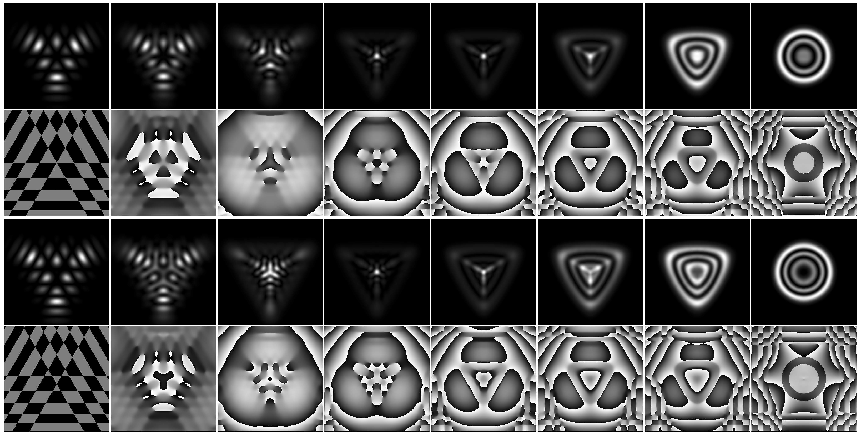
Figure 2.
Experimental set-up: L is laser, is microlens , is lens with mm, is lens with mm, is video camera VSTT-252.
Figure 2.
Experimental set-up: L is laser, is microlens , is lens with mm, is lens with mm, is video camera VSTT-252.
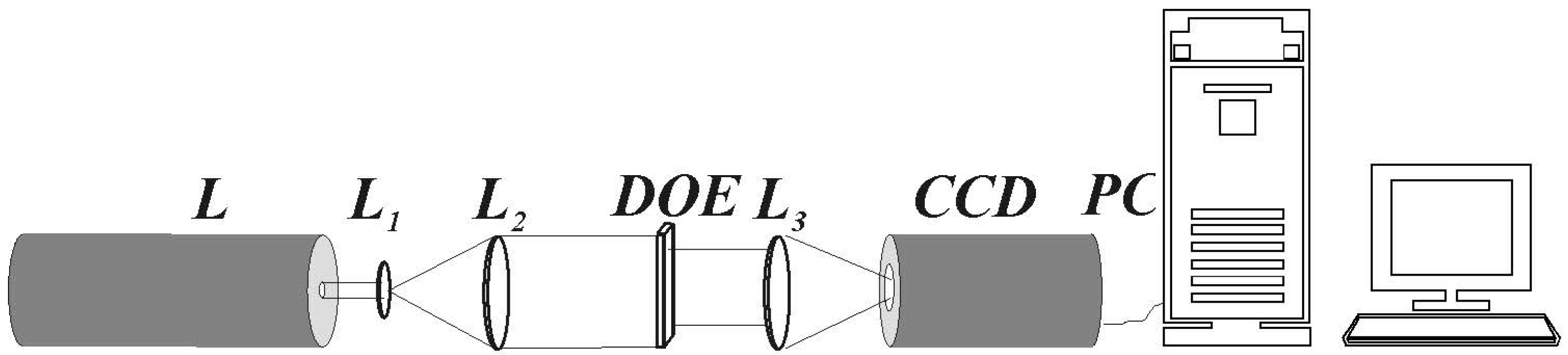
Figure 3.
Numerically evaluated intensity (a) and phase (b) of the input three-Airy beam. Phase of an optical element with encoded amplitude for the formation of a three-Airy beam at (c) and (d).
Figure 3.
Numerically evaluated intensity (a) and phase (b) of the input three-Airy beam. Phase of an optical element with encoded amplitude for the formation of a three-Airy beam at (c) and (d).
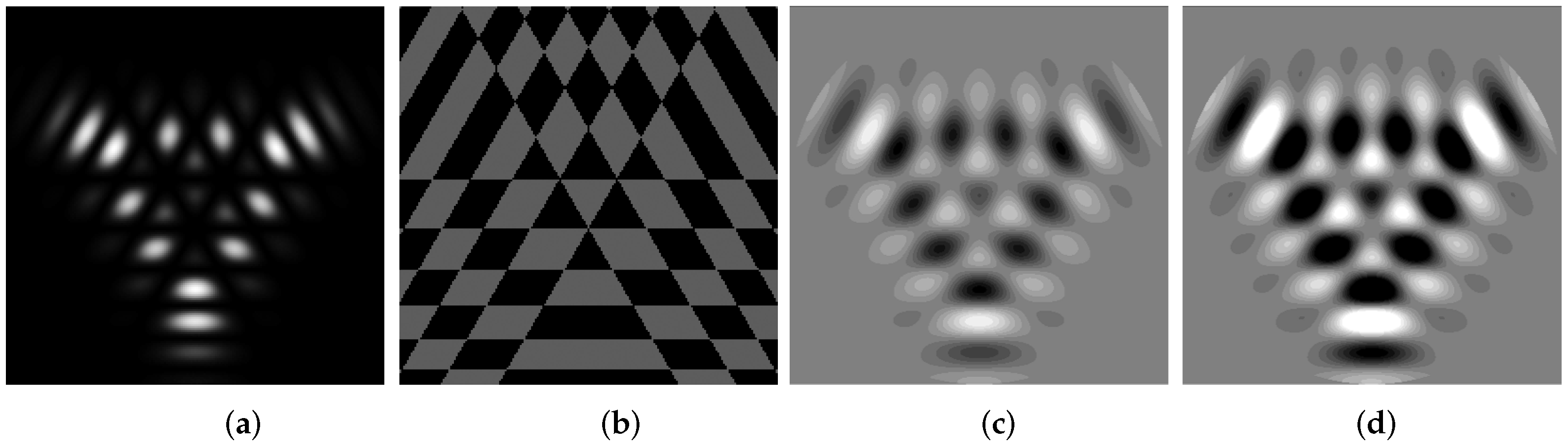
Figure 4.
Surface shape of the coded section of the DOE microrelief (a), surface shape of the uncoded section of the DOE microrelief (b).
Figure 4.
Surface shape of the coded section of the DOE microrelief (a), surface shape of the uncoded section of the DOE microrelief (b).
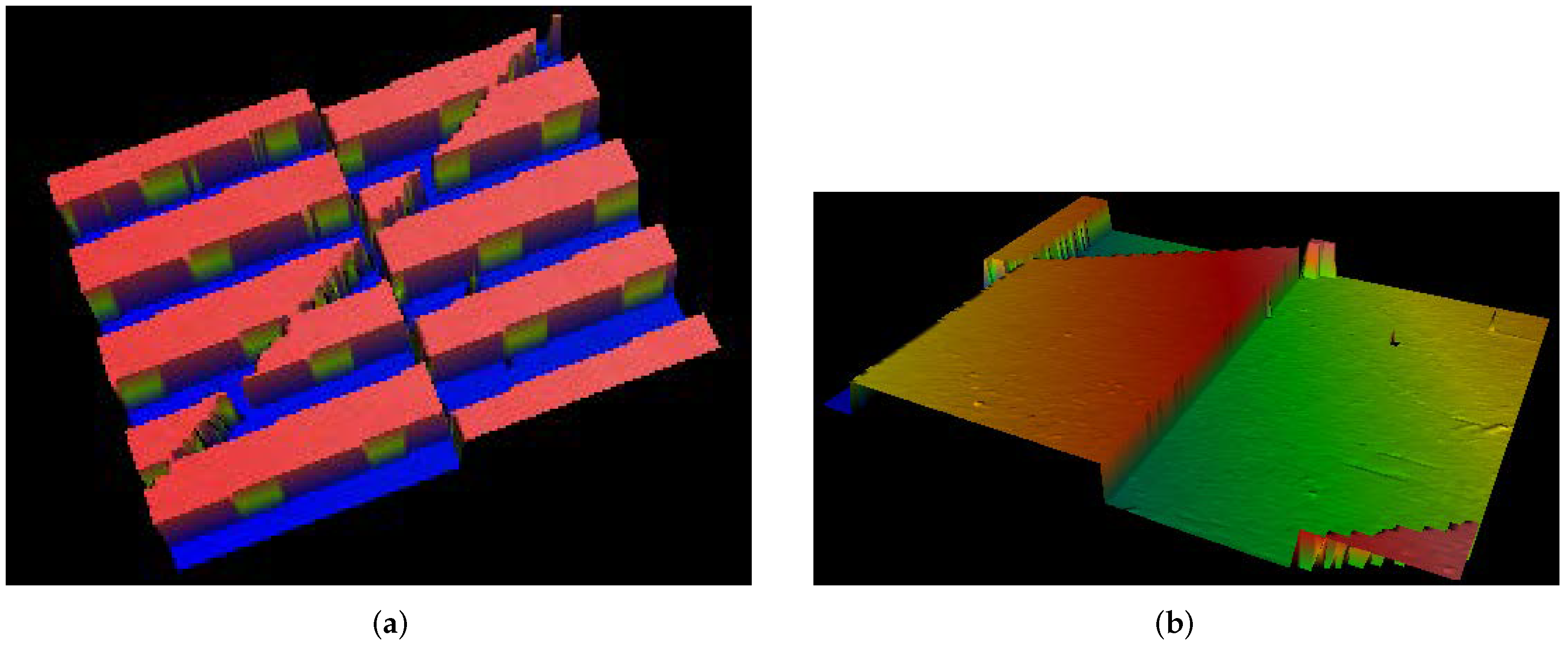
Figure 5.
Intensity distribution of three-Airy beam for the shift parameter at various distances from the input plane: numerical simulations (top row) and results of optical experiment (bottom row).
Figure 5.
Intensity distribution of three-Airy beam for the shift parameter at various distances from the input plane: numerical simulations (top row) and results of optical experiment (bottom row).
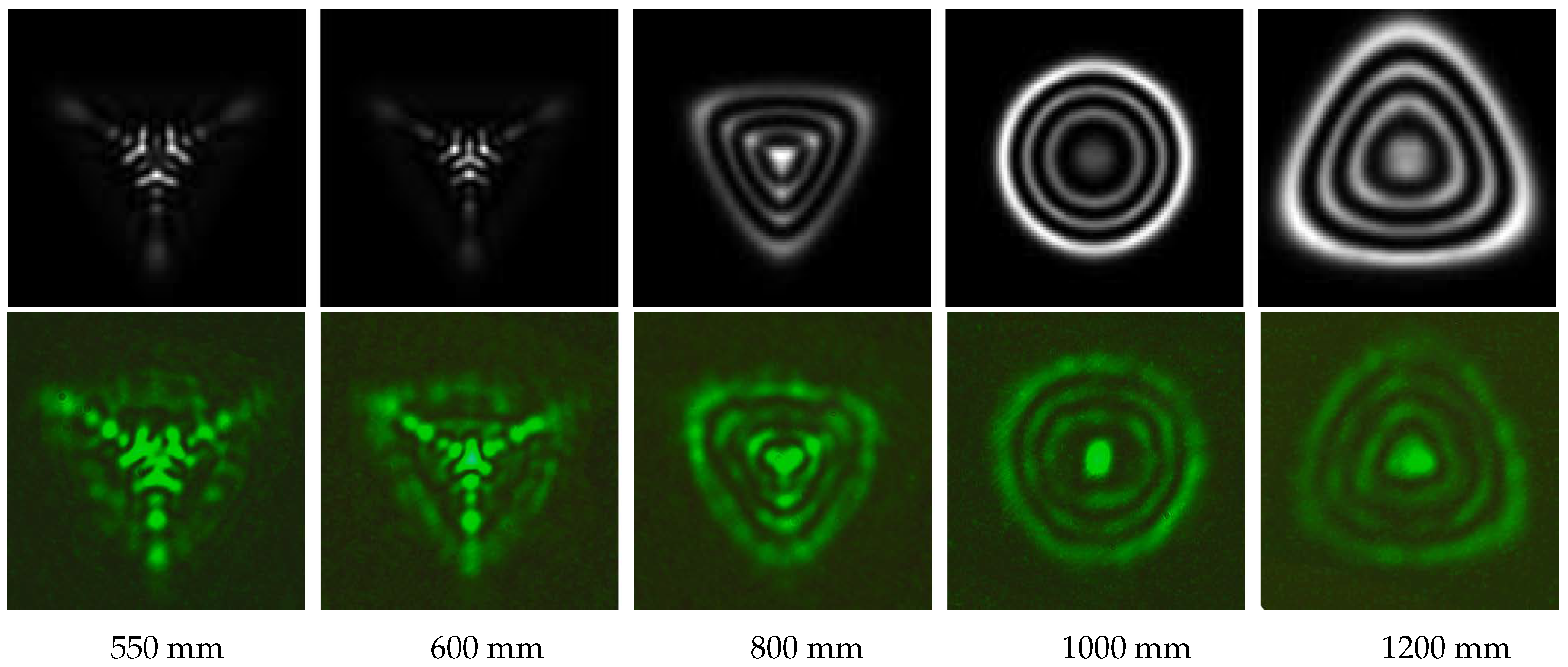
Figure 6.
Intensity distributions versus dimensionless when the shift parameter is , . The global maximum point characterizes the location of the AF plane . If , then there is no such plane. For other ns, the plane exists and the value of increases monotonically with increasing n: 1.842, 3.038, 3.806, 4.389, and 4.868.
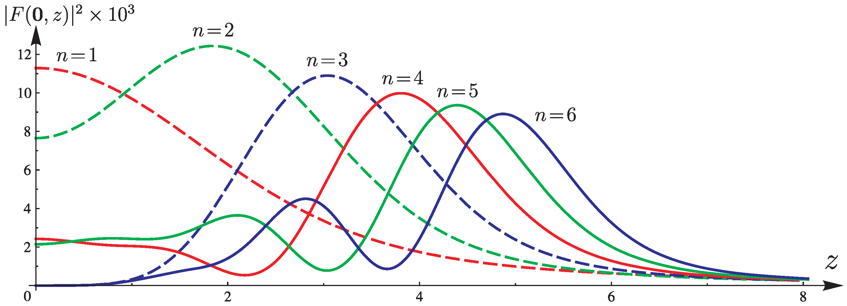
Figure 7.
Intensity distributions versus dimensionless when the shift parameter is , (red), 120 (green), and 140 (blue). Here, , , and , respectively.
Figure 7.
Intensity distributions versus dimensionless when the shift parameter is , (red), 120 (green), and 140 (blue). Here, , , and , respectively.
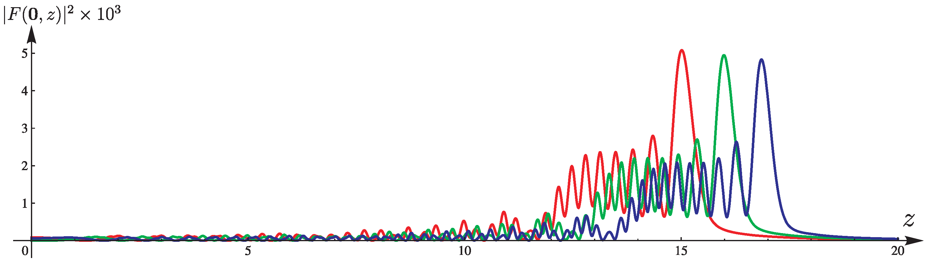
Figure 8.
Left: intervals in for which there is a solution to Equation (25). Right: caustic , , , obtaining from Equations (20)–(22) with . Callout: a zoomed-in area around the origin shows the caustic point, which exists only in the AF plane.

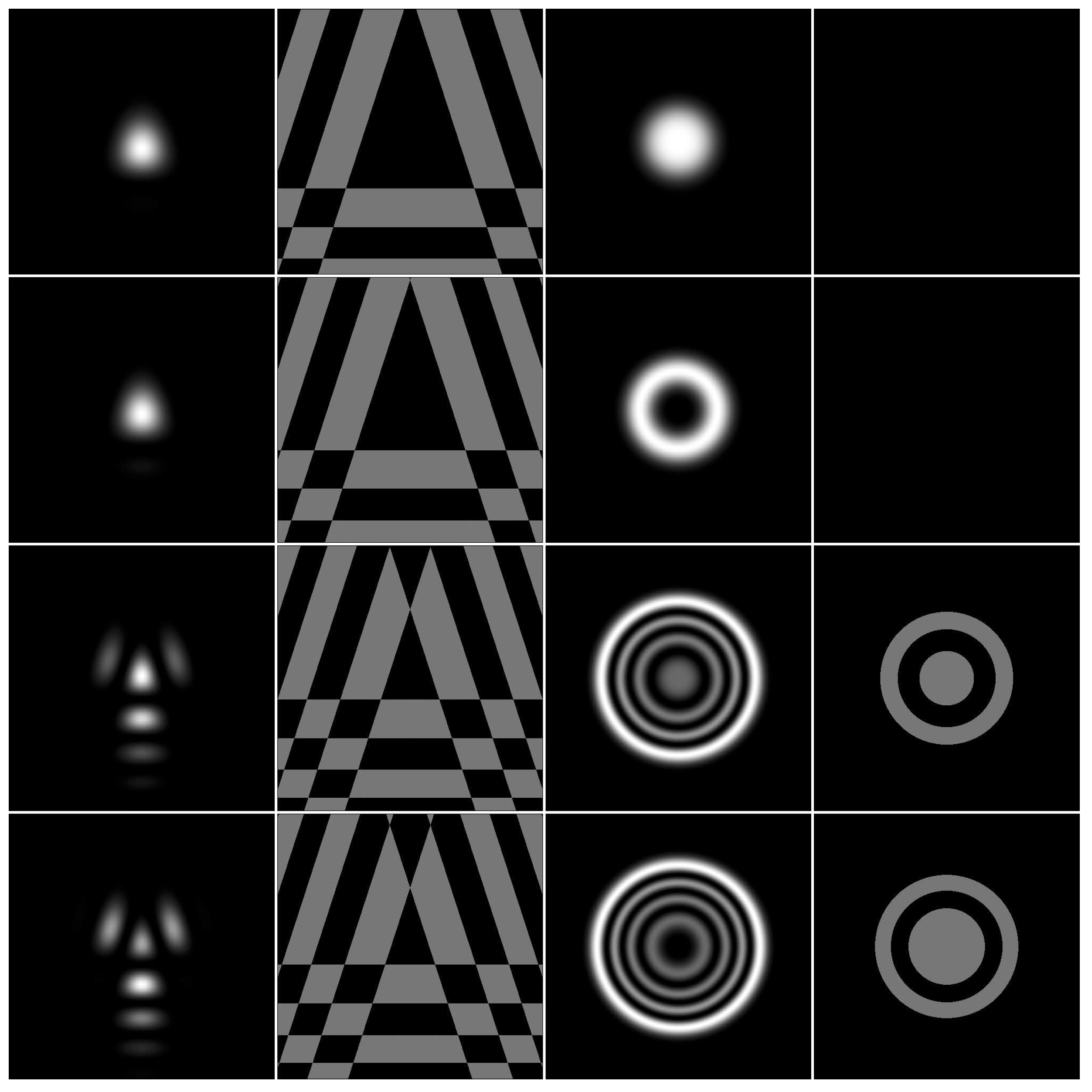
Figure 9.
Numerically evaluated intensity and phase (without cubic component) distributions of the three-Airy beam of infinite energy and of its Fourier image (from left to right). All frames are shown in the square , where .
Figure 9.
Numerically evaluated intensity and phase (without cubic component) distributions of the three-Airy beam of infinite energy and of its Fourier image (from left to right). All frames are shown in the square , where .

Figure 10.
Numerically evaluated intensity and phase (without cubic component) distributions of the three-Airy beam of finite energy and of its Fourier image (from left to right) for the shift parameters (from top to bottom). All frames are shown in the square , where .
Figure 10.
Numerically evaluated intensity and phase (without cubic component) distributions of the three-Airy beam of finite energy and of its Fourier image (from left to right) for the shift parameters (from top to bottom). All frames are shown in the square , where .
Disclaimer/Publisher’s Note: The statements, opinions and data contained in all publications are solely those of the individual author(s) and contributor(s) and not of MDPI and/or the editor(s). MDPI and/or the editor(s) disclaim responsibility for any injury to people or property resulting from any ideas, methods, instructions or products referred to in the content. |
© 2024 by the authors. Licensee MDPI, Basel, Switzerland. This article is an open access article distributed under the terms and conditions of the Creative Commons Attribution (CC BY) license (https://creativecommons.org/licenses/by/4.0/).
Share and Cite
MDPI and ACS Style
Abramochkin, E.G.; Khonina, S.N.; Skidanov, R.V. Three-Airy Beams, Their Propagation in the Fresnel Zone, the Autofocusing Plane Location, as Well as Generalizing Beams. Photonics 2024, 11, 312. https://doi.org/10.3390/photonics11040312
AMA Style
Abramochkin EG, Khonina SN, Skidanov RV. Three-Airy Beams, Their Propagation in the Fresnel Zone, the Autofocusing Plane Location, as Well as Generalizing Beams. Photonics. 2024; 11(4):312. https://doi.org/10.3390/photonics11040312
Chicago/Turabian StyleAbramochkin, Eugeny G., Svetlana N. Khonina, and Roman V. Skidanov. 2024. "Three-Airy Beams, Their Propagation in the Fresnel Zone, the Autofocusing Plane Location, as Well as Generalizing Beams" Photonics 11, no. 4: 312. https://doi.org/10.3390/photonics11040312
Note that from the first issue of 2016, this journal uses article numbers instead of page numbers. See further details here.