Simulation Analysis of an Atmospheric Turbulence Wavefront Measurement System
by
 ,
,
Gangyu Wang
1,2,3 ,
,
Laian Qin
1,3,
Yang Li
1,2,3,
Yilun Cheng
1,2,3,
Xu Jing
1,3,
Gongye Chen
1,2,3 and
Zaihong Hou
1,3,* 1
Key Laboratory of Atmospheric Optics, Anhui Institute of Optics and Fine Mechanics, Hefei Institutes of Physical Science, Chinese Academy of Sciences, Hefei 230031, China
2
Science Island Branch of Graduate School, University of Science and Technology of China, Hefei 230026, China
3
Advanced Laser Technology Laboratory of Anhui Province, Hefei 230037, China
*
Author to whom correspondence should be addressed.
Photonics 2024, 11(4), 383; https://doi.org/10.3390/photonics11040383
Submission received: 19 March 2024
/
Revised: 12 April 2024
/
Accepted: 17 April 2024
/
Published: 18 April 2024
(This article belongs to the Special Issue Optical Imaging and Measurements)
Abstract
:In this paper, a turbulent wavefront measurement model based on the Hartmann system structure is proposed. The maximum recognizable mode number of different lens units is discussed, and the influence of different lens array arrangements on the accuracy of turbulent wavefront reconstruction is analyzed. The results indicate that the increase in the aberration order of the turbulent wavefront has a certain influence on the reconstruction ability of the system. Different lens arrangements and number of lens units will lead to the effective reconstruction of different final mode orders. When using a 5 × 5 lens array arrangement and a hexagonal arrangement of 19 lenses, the maximum order of turbulent wavefront aberrations allowing for effective reconstruction was 25. When the sparse arrangement of 25 lenses or the sparse arrangement of 31 lenses was used, the maximum order allowing for effective reconstruction was 36. If the aberration composition of the turbulent wavefront contained higher-order aberrations, the system could not accurately measure the turbulent wavefront. When the order of the aberrations of the turbulent wavefront was low, the turbulent wavefront could be measured by the lens arrangement with fewer lens units, and the wavefront reconstruction accuracy was close to the measurement results obtained when more lens units were used.
1. Introduction
Turbulence has long been considered one of the most important factors limiting the performance of optical systems in the atmospheric environment [1]. Monitoring the level of optical turbulence in the atmosphere is of great significance for estimating its impact on the functions of optoelectronic devices and systems operating through the atmosphere [2,3,4]. In order to overcome the interference of atmospheric turbulence, large ground-based astronomical telescopes have been equipped with adaptive optical systems in astronomical imaging observations [5,6]. When the laser is transmitted in the atmosphere, it may be affected by turbulence disturbance, molecular absorption, etc., which makes it difficult for the measurement system to accurately obtain the beam parameters at the exit of the laser system [7,8]. Therefore, the analysis of the wavefront after the influence of turbulence helps us to obtain more realistic optical system parameters.
The wavefront detector is one of the key components of adaptive optics systems and can measure the dynamic error of the atmospheric turbulence wavefront in real time. The Shack–Hartmann wavefront sensor (SHWFS) is a commonly used wavefront sensor [9,10,11]. It can measure the wavefront phase of atmospheric turbulence by measuring the slope ϕx, ϕy of the atmospheric turbulence phase ϕ(x, y) in real time through a regularly arranged lens array. Rodolphe [12] proposed a method to generate turbulence measurements using the Shack–Hartmann wavefront sensor. This method takes into account the spatial and temporal statistical characteristics of the slope so that the turbulent wavefront gradient and time series corresponding to the natural guide star and the laser guide star can be generated according to the frozen flow model. Ryan [13] designed a Shack–Hartmann image motion monitor to achieve a 24 h continuous vertical monitoring of atmospheric optical turbulence. Eric [14] believes that the perturbation of the wavefront phase can be measured by a Hartmann wavefront sensor (H-WFS), and then these measurements can be used to directly characterize atmospheric turbulence. However, most of researchers’ work on atmospheric turbulence consists of direct measurements and analyses [15,16,17,18]. Research on the aberrations of atmospheric turbulence, especially high-order aberrations, is relatively scarce. Especially when the Hartmann system structure is used to measure turbulence, the influence of different lens array arrangements on the measurement results still lacks systematic research.
In this paper, a turbulence wavefront measurement model based on the Hartmann system structure is proposed, which can measure and analyze the atmospheric turbulence wavefront under different lens arrangements. At the same time, the wavefront of large-aperture and high-power laser beams propagating through the atmosphere can also be analyzed. According to the correspondence between Zernike polynomials and Seidel aberrations, the turbulent wavefront can be decomposed into multiple single aberrations from low order to high order. In this paper, lens array models with uniform arrangement and sparse arrangement are established. The maximum number of identifiable modes of different lens units is discussed, and the influence of different lens array arrangements on the accuracy of turbulent wavefront reconstruction is analyzed. The results show that the maximum identifiable mode order of the system for the turbulent wavefront is related to the number of sub-lenses in the lens array. Increasing the number of sub-lenses in the lens array can achieve the measurement of a turbulent wavefront with higher-order aberrations. When the order of the aberrations of the turbulent wavefront is low, the turbulent wavefront can be measured by the lens arrangement with fewer lens units, and the wavefront reconstruction accuracy is relatively high.
2. Methodology
2.1. Wavefront Generation
At present, the wavefronts that have been improved in this system model include distorted wavefronts through atmospheric turbulence, dynamic random wavefronts, function-modulated wavefronts, static wavefronts, and plane wavefronts (whose amplitude is 1).
The generation methods of the Kolmogorov turbulence random phase screen include the power spectrum inversion method, the Zernike polynomial method, the random midpoint displacement method, and so on [19,20]. In simulations, the Zernike polynomial method is used to generate the phase screen. The random phase screen generated by this method is non-correlated in the time dimension and can be used for the statistical analysis of multi-frame image data [21]. The low spatial frequency component is consistent with the theoretical value, and the high spatial frequency component gradually improves with the increase in Zernike order. In simulations, the Karhunen–Loeve (K-L) function is used to quickly construct the wavefront [11,22,23,24]. The wavefront φ(r) affected by atmospheric turbulence can be expressed as a two-dimensional function that obeys certain known modes and statistical laws, that is, the two-dimensional form of Zernike polynomials [25]:
where l is the number of modes, is the coefficient of the kth Zernike polynomial, and is the kth Zernike polynomial. Noll derived the covariance of any two Zernike polynomial coefficients from the perspective of energy, which can be expressed as [26]:
where and are the radial frequency numbers of and respectively, and are any two coefficients of Zernike polynomials, D and are the aperture of the telescope and the atmospheric coherence length, respectively, is the gamma function, and and can be expressed as:
where and are the angular frequency numbers of and , respectively, denotes that the polynomials of order and have the same parity, is logic and symbol, and is logic or symbol. From Equations (2)–(4), the covariance matrix of Zernike polynomial coefficients of any order can be obtained, and there is a correlation between Zernike polynomial coefficients. To obtain the turbulent wavefront, Zernike polynomials need to be converted. In the simulation, the K-L function is used to expand the wavefront. The polynomial coefficients are statistically independent, and the Zernike polynomial coefficient matrix can be obtained by conversion.
A random wavefront that does not conform to the statistical law of turbulence can be directly generated by Equation (1). The Zernike coefficient is a pseudo-random number uniformly distributed in the range of (−1, 1). The Zernike coefficients between frames are randomly independent, and the order of Zernike polynomials can be set arbitrarily [27].
2.2. Wavefront Reconstruction Algorithm
The commonly used wavefront reconstruction methods in adaptive optics include the region method, the Zernike mode method, and the direct slope method. In this paper, the Zernike mode method was used for wavefront reconstruction. The phase distribution of the wavefront can be expressed by Equation (1). The wavefront reconstruction calculation of the Zernike mode method can be expressed in the form of the following matrix:
where m is the total number of lens elements, N is the number of Zernike polynomials, and and are the average wavefront slope of the Nth Zernike polynomial in the mth lens region in the x and y directions, respectively, which can be simplified as:
Here, G is the calculated wavefront slope matrix, Z is the 2 m × N reconstruction matrix, and A is the Zernike polynomial coefficient matrix that we need to calculate. The specific solution of matrix A can be achieved by a matrix operation. In general, twice the total number of lenses is larger than the number of Zernike terms, so the singular value decomposition method can be used to calculate the generalized inverse matrix Z+ of Z. The matrix A is determined by
After the coefficient matrix is calculated, the wavefront can be reconstructed by substituting it back into Equation (1).
2.3. Evaluation Method of Wavefront Reconstruction Accuracy
In this paper, we used the root-mean-square error (RMSE) as the standard to measure the accuracy of the wavefront reconstruction. The RMSE represents the root-mean-square value of the wavefront residual; the smaller the value, the higher the accuracy of the restoration. The phase information of a residual wavefront is obtained by subtracting the reconstruction wavefront and the incident wavefront, and then the RMSE is calculated. The calculation formula is:
where is the original wavefront, is the recovery wavefront, and N is the total number of sampling points.
3. Numerical Simulation Conditions
3.1. Simulation System Parameters
Under the same arrangement, the wavefront reconstruction accuracy of the system increases with the increase in the duty factor of the lens array. When the duty factor of the lens array is about 0.8, the wavefront reconstruction accuracy of the system is moderately different from that obtained when the duty factor of the lens array is 1 [28]. On the premise of using the smallest lens size combination to detect the largest distortion wavefront, we chose a duty factor of the system lens array of 0.8.
In addition, since the Zernike mode method is based on centroid detection when reconstructing the wavefront, the centroid detection accuracy is particularly important. To improve the accuracy of the sub-spot centroid measurement, it is especially necessary to ensure that the sub-spot size in the detection surface corresponds to a large number of pixels. In this system, the minimum pixel area covered by the spot was set to 10 pixel × 10 pixel to ensure the accuracy of the centroid measurement. According to Equation (9), the number of pixels occupied by the spot can be determined by:
where P = 4.5 μm is the pixel size, and λ = 1064 nm is the wavelength; if p ≥ 10, then f ≥ 20 d. However, in addition to considering the number of pixels in the imaging spot, the selection of the lens parameters should also consider whether the camera pixel resolution can achieve the effective detection of wavefront distortion under different wavefront distortion degrees.
Figure 1 shows the imaging properties of the sub-lens with a plane wavefront (green parallel line) incident on the lens and focused on the reference spot (green spot). The distorted wavefront (red parallel line) does not have a normal incidence, focusing on the position deviating from the reference spot (red point). The offset angle α can be calculated according to geometric parameters. According to the geometric relationship of the offset angle, the relationship between the wavefront distortion and the detected spot displacement can be derived:
The relationship between the PV (peak–valley) value and the RMS value of the wavefront had to be measured, and its β was determined by simulation. When the PV value of the initial wavefront was 0.6 λ, and the RMS value was about 0.15 λ, the beam quality factor β of the far-field spot was about 1.8. Here, β is an important parameter used to describe the quality of a laser beam. It is usually used to measure the degree of similarity between a laser beam and an ideal Gaussian beam and can also be used to compare the quality difference between different laser beams, defined as the ratio of the actual far-field divergence angle to the reference far-field divergence angle or as the ratio of the actual focused spot radius to the ideal spot radius. Therefore, we set the wavefront PV value of the minimum effective reconstruction to be achieved by the measurement system to about 0.6 λ. If the number of single-row lenses was 5, and the space-occupying factor of the system was 0.8, the wavefront measured by a single lens was about 0.096 λ. According to (10), we can calculate f ≥ 47 d.
When the lens diameter was d = 25.4 mm, the focal length was f ≥ 47 d ≈ 1194 mm. In other words, when the diameter of the selected lens was 25.4 mm, the focal length of the lens had to be adjusted to not less than 1194 mm to meet the measurement requirements of the system. In summary, the main input parameters of the system are shown in Table 1.
3.2. Lens Array Arrangement
In this paper, different turbulent wavefronts were analyzed. It was necessary to consider the influence on the wavefront reconstruction accuracy not only of the number of sub-lenses in the lens array of the measurement system but also of different lens arrangements. Therefore, we propose two lens array layouts: a uniform arrangement and a sparse arrangement. The uniform arrangement included the 5 × 5 lens array arrangement and a 19-lense hexagonal arrangement, and the sparse arrangement included 25 lenses and a 31-lense sparse arrangement. Here, the sparse arrangement was mainly applied to the recovery analysis of higher-order aberrations, because the slope variation of higher-order aberrations was mainly concentrated in the edge of the wavefront. The specific lens array layouts are shown in Figure 2. The red area in the figure is the effective detection range of the wavefront to be measured.
4. Results and Discussion
4.1. Single Aberration Analysis
When using Zernike polynomials to reconstruct the wavefront of a distorted wavefront, mode coupling and confusion need to be considered. Mode coupling is caused by the number of Zernike terms selected in wavefront reconstruction being less than the number of mode terms of the actual distorted wavefront. The reason for mode confusion is that high-order aberrations and low-order aberrations cannot be effectively distinguished within the sub-lens range of the system. Dai [22] and Zhang [29] et al. also discussed the relationship between mode confusion, mode coupling, and the number of Zernike terms used in wavefront reconstruction. By selecting different wavefront reconstruction orders, the corresponding wavefront reconstruction accuracy and stability curves are obtained, and then the final wavefront reconstruction order is determined by comparison. The turbulence wavefront is mainly composed of low-order Zernike polynomials, and the proportion of high-order Zernike polynomials is very small. Therefore, the first 28 Zernike polynomials excluding piston and tilt were selected for wavefront reconstruction. To avoid mode coupling, the order of the mode wavefront reconstruction we selected was the same as the order of the actual aberration. According to the four kinds of lens array arrangement described in Section 3.2, the reconstruction analysis of each single aberration order was carried out. The simulation results are shown in Figure 3, and the statistical values of the reconstruction accuracy for the different orders of single aberrations of the four kinds of lens array arrangement are shown in Table 2.
In order to facilitate the exposition, in the following, the lens arrangements are indicated as 1, 2, 3, 4, corresponding to the 5 × 5 lens array arrangement, the hexagonal arrangement of 19 lenses, the sparse arrangement of 25 lenses, and the sparse arrangement of 31 lenses, respectively.
Combining Figure 3 and Table 2, it can be seen that among the four lens array arrangements, the lens arrangement 1 and the lens arrangement 4 allowed for better reconstruction accuracy for the first 28 single aberrations. This is because the number of lens units in these two arrangements was relatively large. The reconstruction accuracy for single aberrations of the lens arrangement 1 was better than that achieved by the lens arrangement 3. The reason is that the number of lens units in the two arrangements was close, and the lens units in the former were arranged more closely. According to the results obtained with arrangement 3 and arrangement 4, we concluded that a sparse arrangement does not provide much advantage in low-order aberration reconstruction. When the number of lens units is relatively small, the aberration recovery ability of a sparse arrangement is not as good as that of a uniform arrangement. However, when the number of sparsely arranged lens units is large, a sparse arrangement has a good reconstruction effect on the aberrations of the turbulent wavefront, especially on high-order aberrations. This is because the higher the order of the turbulent wavefront aberrations, the larger their proportion at the wavefront edge. Figure 4 shows the reconstruction results in the presence of some high-order aberrations when using the lens arrangement 4.
4.2. Maximum Recognizable Mode Order of the System
The wavefront reconstruction accuracy and stability are used to evaluate the wavefront reconstruction process when considering different mode reconstruction orders for wavefront reconstruction. The wavefront reconstruction accuracy evaluation method was described in detail in Section 2.3. Stability means that the anti-noise interference ability of the wavefront reconstruction process can be evaluated by the condition number of the reconstruction matrix [30,31]. The condition number is defined as:
where and represent the maximum and the minimum singular values of the reconstruction matrix Z, respectively. The relationship between the Zernike mode coefficient fluctuation ΔA of the reconstructed wavefront and the slope measurement disturbance ΔG is as follows:
The above formula shows that the larger the condition number, the greater the fluctuation of the Zernike mode coefficients of the reconstructed wavefront caused by the slope measurement error.
According to Figure 3, the aberration recovery accuracy of the four arrangements showed an upward trend after the 21st order, which indicated that the increase in the aberration order had a certain degree of influence on the recovery ability of the system. Therefore, we continued to increase the order of the turbulent wavefront aberrations to be measured and analyzed the maximum order of recognizable modes that could be achieved by the different arrangements. In addition, the condition numbers of the four arrangements for different wavefronts are reported to judge whether the recovery results were reliable. The turbulent wavefront aberration reconstruction accuracy of the different examined arrangements is shown in Figure 5a, and the curve displaying the condition number changing with the increase in the aberration order is shown in Figure 5b.
According to Figure 5, when the order of the turbulent wavefront aberrations exceeded 25, the condition number of the lens arrangements 1 and 2 increased sharply, and the wavefront recovery accuracy decreased rapidly, which means that the wavefront reconstruction ability was poor. Therefore, we determined that the maximum order of turbulent wavefront aberrations for the lens arrangements 1 and 2 allowing for achieving effective reconstruction was 25. According to Figure 5a, we could also conclude that in order to ensure a high reconstruction accuracy, the order of turbulent wavefront aberrations with the lens arrangements 1 and 2 should not exceed 21. With the lens arrangements 3 and 4, the reconstruction accuracy and stability of the turbulent wavefront composed of the first 36 aberrations were relatively good. In order to continue to explore the maximum possible order of these two arrangements allowing for effective wavefront reconstruction, we continued to increase the constituent aberrations of the turbulent wavefront. Further simulation results are shown in Figure 6. According to the above analysis and as shown in Figure 6, the maximum order allowing for effective reconstruction was 36 with the lens arrangements 3 and 4. This further illustrates that different lens arrangements and different numbers of lens units in the turbulent wavefront reconstruction system will lead to effective recovery in the presence of different aberration orders.
4.3. Turbulent Wavefront Analysis
The third section of this paper discusses the accuracy of turbulent wavefront aberration reconstruction under different lens arrangements and the maximum order allowing for effective reconstruction that can be achieved with the various arrangements. The atmospheric turbulence wavefront in the actual measurement presented mixed aberrations. According to the Equations (2)–(5) in Section 2.2, we can obtain a series of random turbulent wavefronts. In order to facilitate the comparison of the reconstruction ability of the four arrangements in the presence of mixed aberrations, we generated two different sets of turbulent wavefronts. In one group, the maximum order of aberrations that constituted the turbulent wavefront was 28, and the aberration coefficients of the orders from the 22nd to the 28th were much smaller than the remaining aberration coefficients. The other group of turbulent wavefront only retained the wavefront aberration coefficients of the first 21 orders of the previous group. Figure 7 shows the RMS value curve of the generated turbulent wavefront aberrations.
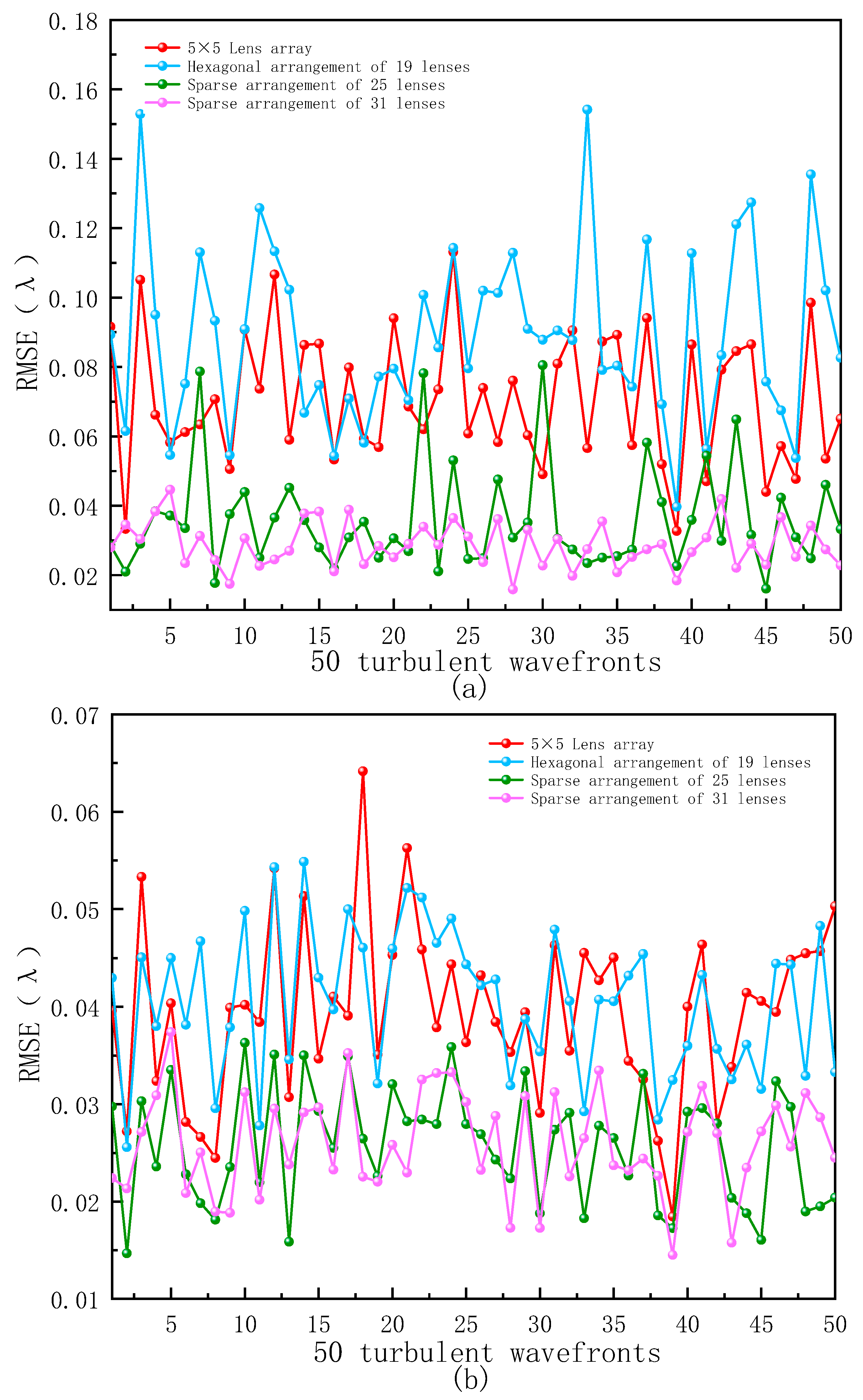
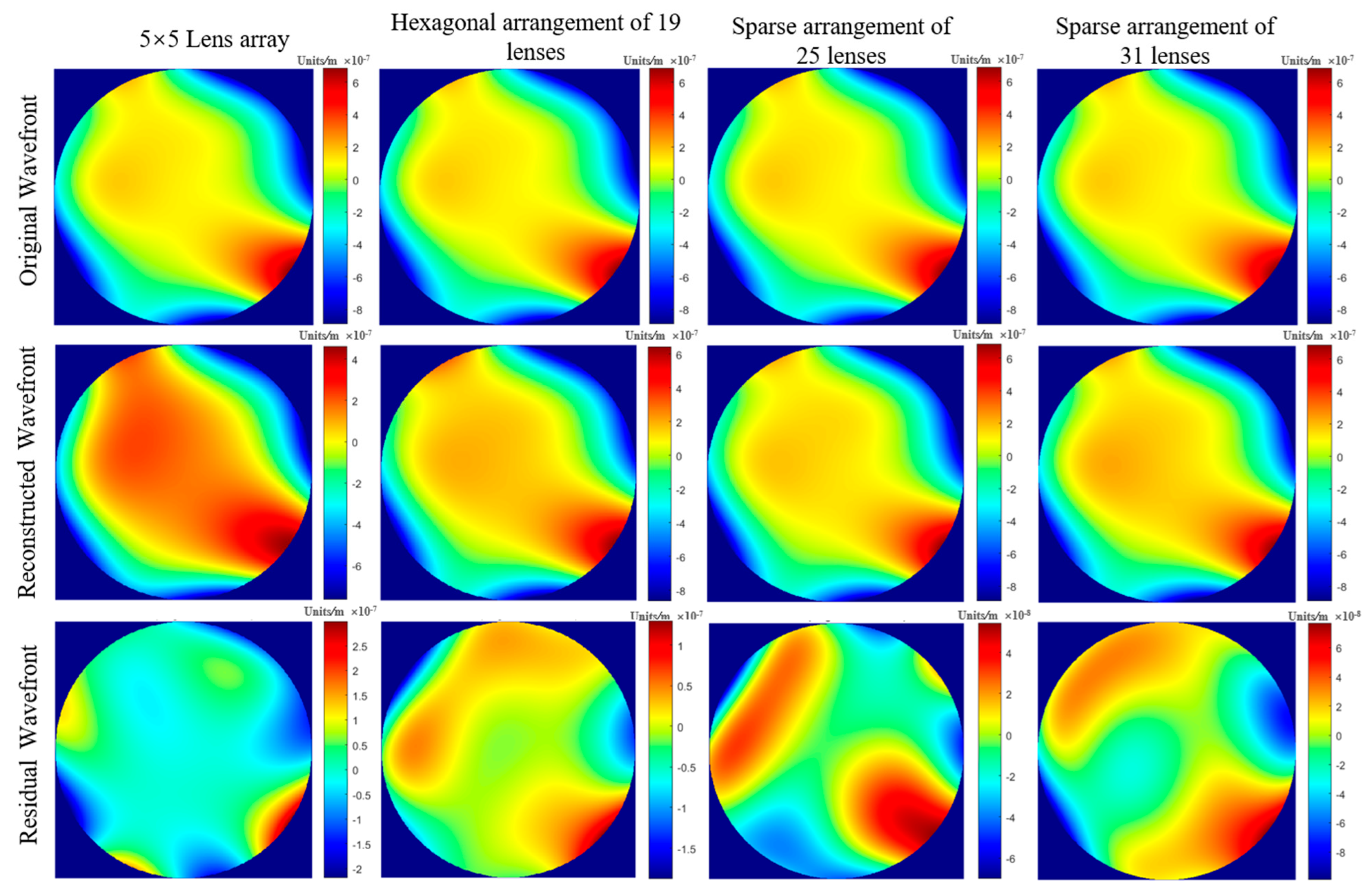
The generated wavefront was processed and examined by the lens array systems to obtain a reconstructed wavefront, and then the wavefront reconstruction accuracy was calculated. Figure 8 shows one of the calculation examples. The same turbulent wavefront was reconstructed by the above four arrangements. The measured turbulent wavefront PV value was 1.56 λ, and the RMS value was 0.26 λ. The turbulent wavefront reconstruction accuracy of the four arrangements is shown in Figure 9.
According to Figure 9, we can conclude that for general turbulent wavefronts, the number of sub-lenses in the lens array is a major factor limiting wavefront measurements. Due to the relatively small number of lens units, the maximum number of modes that could be effectively identified was also relatively low. This caused the system to lose the ability to measure the turbulent wavefront when higher-order aberrations were present in. The reconstruction results when using the lens arrangements 3 and 4 proved that increasing the number of sub-lenses in the lens array can allow for the measurement of a turbulent wavefront with higher-order aberrations. As shown in Figure 9b, when the aberration order of the turbulent wavefront was low, the lens arrangement with fewer lenses could be used to measure the turbulent wavefront, and the wavefront reconstruction accuracy was less different from that achieved when the number of lenses was large, compared to the previous situation.
5. Conclusions
In this paper, a turbulent wavefront measurement model based on the Hartmann system structure is proposed, which can measure and analyze atmospheric turbulence wavefronts using different lens arrangements. Four lens array models with uniform and sparse arrangements were established. The maximum identifiable aberration order for different lens numbers was discussed, and the influence of different lens array arrangements on the accuracy of turbulent wavefront reconstruction was analyzed. The results showed that the increase in the aberration order of the turbulent wavefront had a certain influence on the reconstruction ability of the system. When the system contained a 5 × 5 lens array arrangement or a hexagonal arrangement of 19 lenses, the maximum order of turbulent wavefront aberration allowing for effective reconstruction was 25. In order to ensure a high reconstruction accuracy, the reconstruction order of turbulence wavefront aberrations should not exceed 21. When the system contained a 25-lense sparse arrangement or a 31-lense sparse arrangement, the reconstruction accuracy and stability of the turbulent wavefront composed of the first 36 aberrations were relatively good. This also proved that different lens arrangements and different numbers of lenses in the turbulence wavefront reconstruction system will lead to effective reconstruction in the presence of aberration of different orders.
When the aberration composition of the turbulent wavefront contained higher-order aberrations, the system could not accurately measure the turbulent wavefront. Increasing the number of sub-lenses in the lens array could achieve the measurement of a turbulent wavefront with higher-order aberrations. When the aberration order of the turbulent wavefront was low, the lens arrangement with a small number of lens units could be used to measure the turbulent wavefront.
The turbulence wavefront measurement model proposed in this paper provides a new idea and method for atmospheric turbulence measurement. It is effective for the analysis of the operating performance of optical systems affected by turbulence.
Author Contributions
Conceptualization, G.W.; methodology, Z.H. and L.Q.; software, G.W., G.C. and Y.L.; writing—original draft preparation, G.W., L.Q. and X.J.; writing—review and editing, G.W., Y.C. and L.Q. All authors have read and agreed to the published version of the manuscript.
Funding
This research was funded by the National Natural Science Foundation of China (Grant No. 41875033).
Institutional Review Board Statement
Not applicable.
Informed Consent Statement
Not applicable.
Data Availability Statement
Data are available upon request.
Acknowledgments
The authors are thankful to their colleagues from AIOFM—Feng He, Xiaoshan Yuan, Zeli Tang, and Lijun Chen—for the help in this study.
Conflicts of Interest
The authors declare no conflicts of interest.
References
- Lukin, V.P.; Bol’basova, L.A.; Nosov, V.V. Comparison of Kolmogorov’s and coherent turbulence. Appl. Opt. 2014, 53, B231–B236. [Google Scholar] [CrossRef] [PubMed]
- Wu, G.; Guo, H.; Yu, S.; Luo, B. Spreading and direction of Gaussian–Schell model beam through a non-Kolmogorov turbulence. Opt. Lett. 2010, 35, 715–717. [Google Scholar] [CrossRef]
- Cheng, Z.; He, L.; Zhang, X.; Mu, C.; Tan, M. Autocorrected preconditioning regularization inversion algorithm for an atmospheric turbulence profile. Appl. Opt. 2020, 59, 8773–8788. [Google Scholar] [CrossRef] [PubMed]
- Xu, Z.; Liu, X.; Cai, Y.; Ponomarenko, S.A.; Liang, C. Structurally stable beams in the turbulent atmosphere: Dark and antidark beams on incoherent background [Invited]. J. Opt. Soc. Am. A 2022, 39, C51–C57. [Google Scholar] [CrossRef] [PubMed]
- Lin, X.D.; Xue, C.; Liu, X.Y.; Wang, J.L.; Wei, P.F. Current status and research development of wavefront correctors for adaptive optics. Chin. Opt. 2012, 5, 337–351. [Google Scholar]
- Davis, J.I. Consideration of Atmospheric Turbulence in Laser Systems Design. Appl. Opt. 1966, 5, 139–147. [Google Scholar] [CrossRef] [PubMed]
- Liou, K.N.; Ou, S.-C.; Takano, Y.; Cetola, J. Remote sensing of three-dimensional cirrus clouds from satellites: Application to continuous-wave laser atmospheric transmission and backscattering. Appl. Opt. 2006, 45, 6849–6859. [Google Scholar] [CrossRef] [PubMed]
- Liang, X.; Zhong, M.; Xu, T.; Xiao, J.; Jiao, K.; Wang, X.; Bin, Y.; Liu, J.; Wang, X.; Zhao, Z.; et al. Mid-Infrared Single-Mode Ge-As-S Fiber for High Power Laser Delivery. J. Lightwave Technol. 2022, 40, 2151–2156. [Google Scholar] [CrossRef]
- Bolbasova, L.A.; Gritsuta, A.N.; Kopylov, E.A.; Lavrinov, V.V.; Lukin, V.P.; Selin, A.A.; Soin, E.L. Atmospheric turbulence meter based on a Shack–Hartmann wavefront sensor. J. Opt. Technol. 2019, 86, 426–430. [Google Scholar] [CrossRef]
- McCrae, J.E.; Bose-Pillai, S.; Current, M.; Lee, K.; Fiorino, S. Analysis of Turbulence Anisotropy with a Hartmann Sensor. In Proceeding of the Imaging and Applied Optics 2017, Beijing, China, 4–6 June 2017. [Google Scholar]
- Anzuola, E.; Zepp, A.; Marin, P.; Gladysz, S.; Stein, K. Holographic Wavefront Sensing for Atmospheric Turbulence using Karhunen-Loève Decomposition. In Proceeding of the Imaging and Applied Optics 2016, Heidelberg, Germany, 25–28 July 2016. [Google Scholar]
- Conan, R. Random generation of the turbulence slopes of a Shack–Hartmann wavefront sensor. Opt. Lett. 2014, 39, 1390–1393. [Google Scholar] [CrossRef] [PubMed]
- Griffiths, R.; Osborn, J.; Farley, O.; Butterley, T.; Townson, M.J.; Wilson, R. Demonstrating 24-h continuous vertical monitoring of atmospheric optical turbulence. Opt. Express 2023, 31, 6730–6740. [Google Scholar] [CrossRef]
- Silbaugh, E.E.; Welsh, B.M.; Roggemann, M.C. Characterization of atmospheric turbulence phase statistics using wave-front slope measurements. J. Opt. Soc. Am. A 1996, 13, 2453–2460. [Google Scholar] [CrossRef]
- Joo, J.Y.; Han, S.G.; Lee, J.H.; Rhee, H.-G.; Huh, J.; Lee, K.; Park, S.Y. Development and Characterization of an Atmospheric Turbulence Simulator Using Two Rotating Phase Plates. Curr. Opt. Photon. 2022, 6, 445–452. [Google Scholar]
- Nelson, D.H.; Walters, D.L.; MacKerrow, E.P.; Schmitt, M.J.; Quick, C.R.; Porch, W.M.; Petrin, R.R. Wave optics simulation of atmospheric turbulence and reflective speckle effects in CO2 lidar. Appl. Opt. 2000, 39, 1857–1871. [Google Scholar] [CrossRef] [PubMed]
- Lukin, V.P. Models and measurements of atmospheric turbulence characteristics and their impact on AO design. In Proceeding of the Adaptive Optics 1996, Maui, HI, USA, 8–12 July 1996. [Google Scholar]
- Caldwell, E.D.; Swann, W.C.; Ellis, J.L.; Bodine, M.I.; Mak, C.; Kuczun, N.; Newbury, N.R.; Sinclair, L.C.; Muschinski, A.; Rieker, G.B. Optical timing jitter due to atmospheric turbulence: Comparison of frequency comb measurements to predictions from micrometeorological sensors. Opt. Express 2020, 28, 26661–26675. [Google Scholar] [CrossRef] [PubMed]
- Bol’basova, L.A.; Lukin, V.P. Issues of wavefront tilt measurement. J. Opt. Technol. 2021, 88, 625–629. [Google Scholar] [CrossRef]
- Van Zandt, N.R.; Spencer, M.F.; Fiorino, S.T. Speckle mitigation for wavefront sensing in the presence of weak turbulence. Appl. Opt. 2019, 58, 2300–2310. [Google Scholar] [CrossRef]
- Wei, P.; Li, X.Y.; Luo, X.; Li, J.F. Design and Verification of Digital Simulation Platform for Shack-Hartmann Wavefront Sensors. Chin. J. Lasers 2021, 48, 141–150. [Google Scholar]
- Dai, G.M. Modal compensation of atmospheric turbulence with the use of Zernike polynomials and Karhunen–Loève functions. J. Opt. Soc. Am. A 1995, 12, 2182–2193. [Google Scholar] [CrossRef]
- Zepp, A.; Gladysz, S.; Stein, K.; Osten, W. Optimization of the holographic wavefront sensor for open-loop adaptive optics under realistic turbulence. Part I: Simulations. Appl. Opt. 2021, 60, F88–F98. [Google Scholar] [CrossRef] [PubMed]
- Dai, G.M. Modal wave-front reconstruction with Zernike polynomials and Karhunen–Loève functions. J. Opt. Soc. Am. A 1996, 13, 1218–1225. [Google Scholar] [CrossRef]
- Noll, R.J. Zernike polynomials and atmospheric turbulence. J. Opt. Soc. Am. 1976, 66, 207–211. [Google Scholar] [CrossRef]
- Roddier, N. Atmospheric wavefront simulation using zernike polynomials. Opt. Eng. 1990, 29, 1174–1180. [Google Scholar] [CrossRef]
- Lukin, V.P.; Nosov, E.V.; Nosov, V.V.; Torgaev, A.V. Causes of non-Kolmogorov turbulence in the atmosphere. Appl. Opt. 2016, 55, B163–B168. [Google Scholar] [CrossRef] [PubMed]
- Wang, G.Y.; Hou, Z.H.; Qin, L.A.; Jing, X.; Wu, Y. Simulation Analysis of a Wavefront Reconstruction of a Large Aperture Laser Beam. Sensors 2023, 23, 623. [Google Scholar] [CrossRef] [PubMed]
- Zhang, Q.; Jiang, W.H.; Xu, B. Reconstruction of Turbulent Optical Wavefront Realized by Zernike Polynomial. Opto-Electron. Eng. 1998, 25, 15–19. [Google Scholar]
- Li, J.; Liu, J.; Liu, D.; Tian, W.; Jin, S.; Hu, S.; Guo, J.; Jin, Y. Ultrafast Random Number Generation Based on Random Laser. J. Lightwave Technol. 2023, 41, 5233–5243. [Google Scholar] [CrossRef]
- Twietmeyer, K.; Chipman, R. Condition Number as a Metric for the Effectiveness of Polarimetric Algorithms. In Proceeding of the Frontiers in Optics 2005, San Jose, CA, USA, 18–22 October 2015. [Google Scholar]
Figure 1.
Sub-lens imaging schematic diagram.

Figure 2.
Different lens array arrangements. (a) A 5 × 5 lens array, (b) a hexagonal arrangement of 19 lenses, (c) a sparse arrangement of 25 lenses; (d) a sparse arrangement of 31 lenses.
Figure 2.
Different lens array arrangements. (a) A 5 × 5 lens array, (b) a hexagonal arrangement of 19 lenses, (c) a sparse arrangement of 25 lenses; (d) a sparse arrangement of 31 lenses.
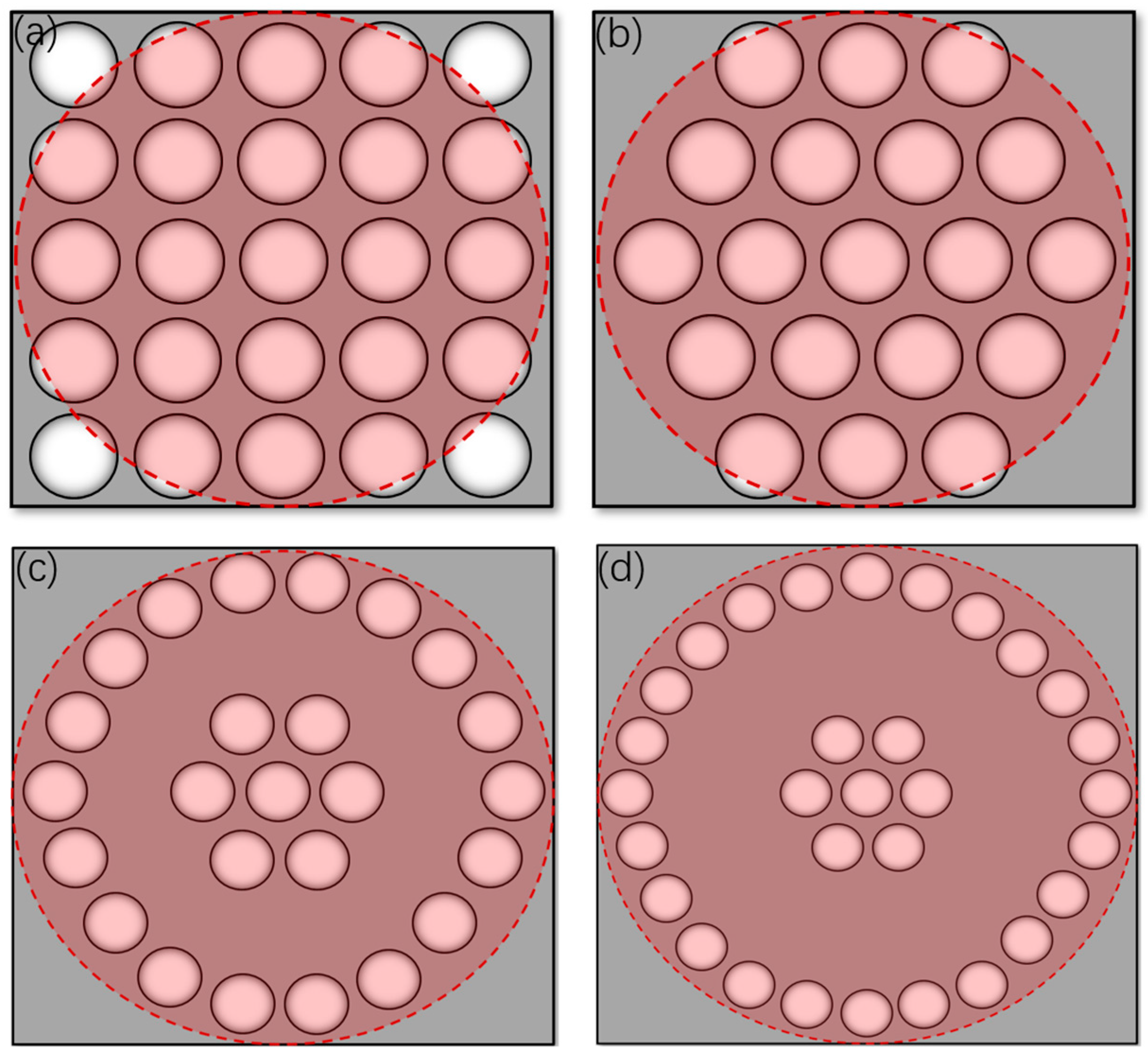
Figure 3.
The reconstruction accuracy for the first 28 orders of single aberrations of different lens arrangements.
Figure 3.
The reconstruction accuracy for the first 28 orders of single aberrations of different lens arrangements.
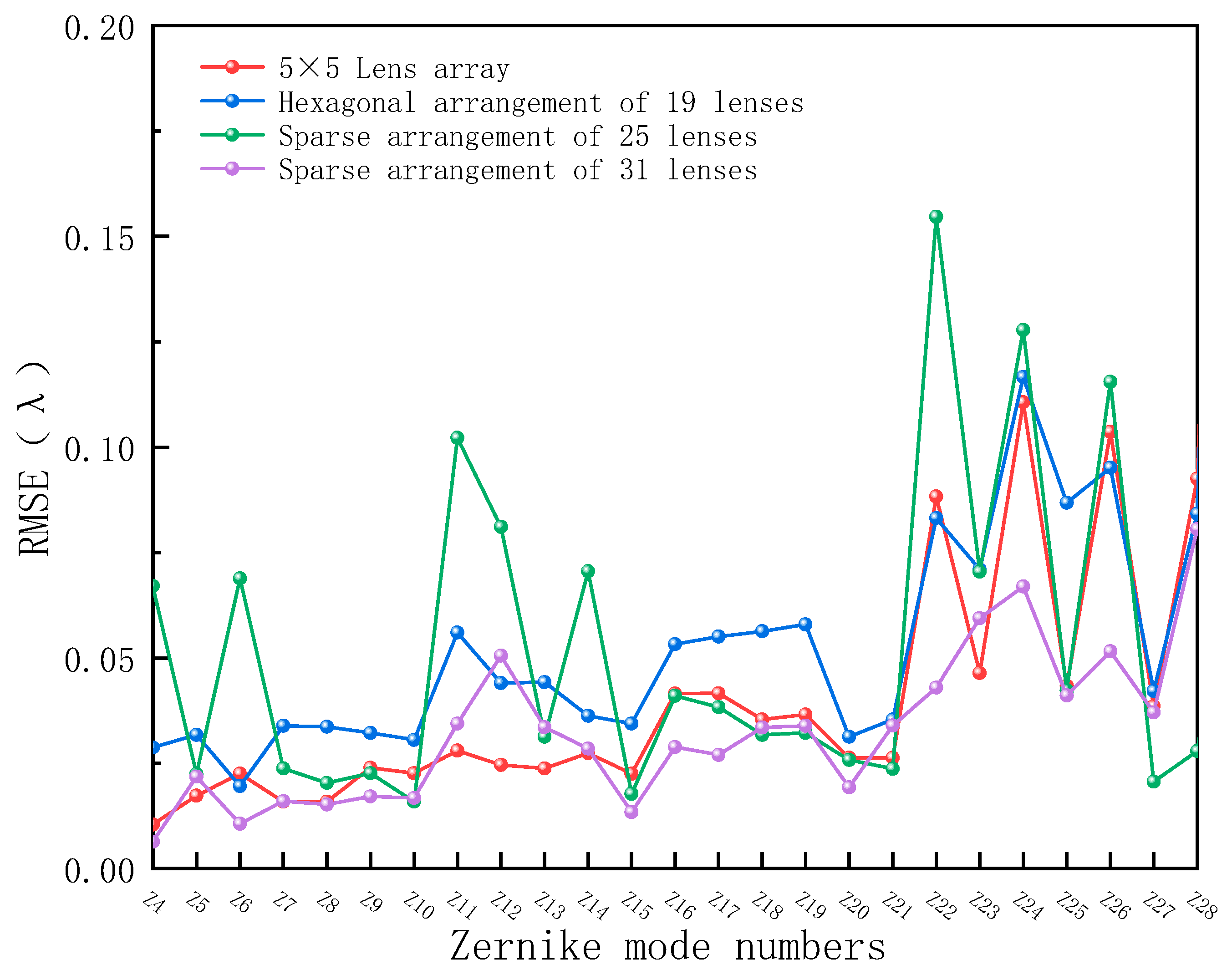
Figure 4.
Wavefront reconstruction of high-order aberrations by a sparse lens arrangement.

Figure 5.
Reconstruction results of a turbulent wavefront by different lens arrangements. (a) Turbulent wavefront reconstruction accuracy, (b) turbulent wavefront reconstruction stability.
Figure 5.
Reconstruction results of a turbulent wavefront by different lens arrangements. (a) Turbulent wavefront reconstruction accuracy, (b) turbulent wavefront reconstruction stability.
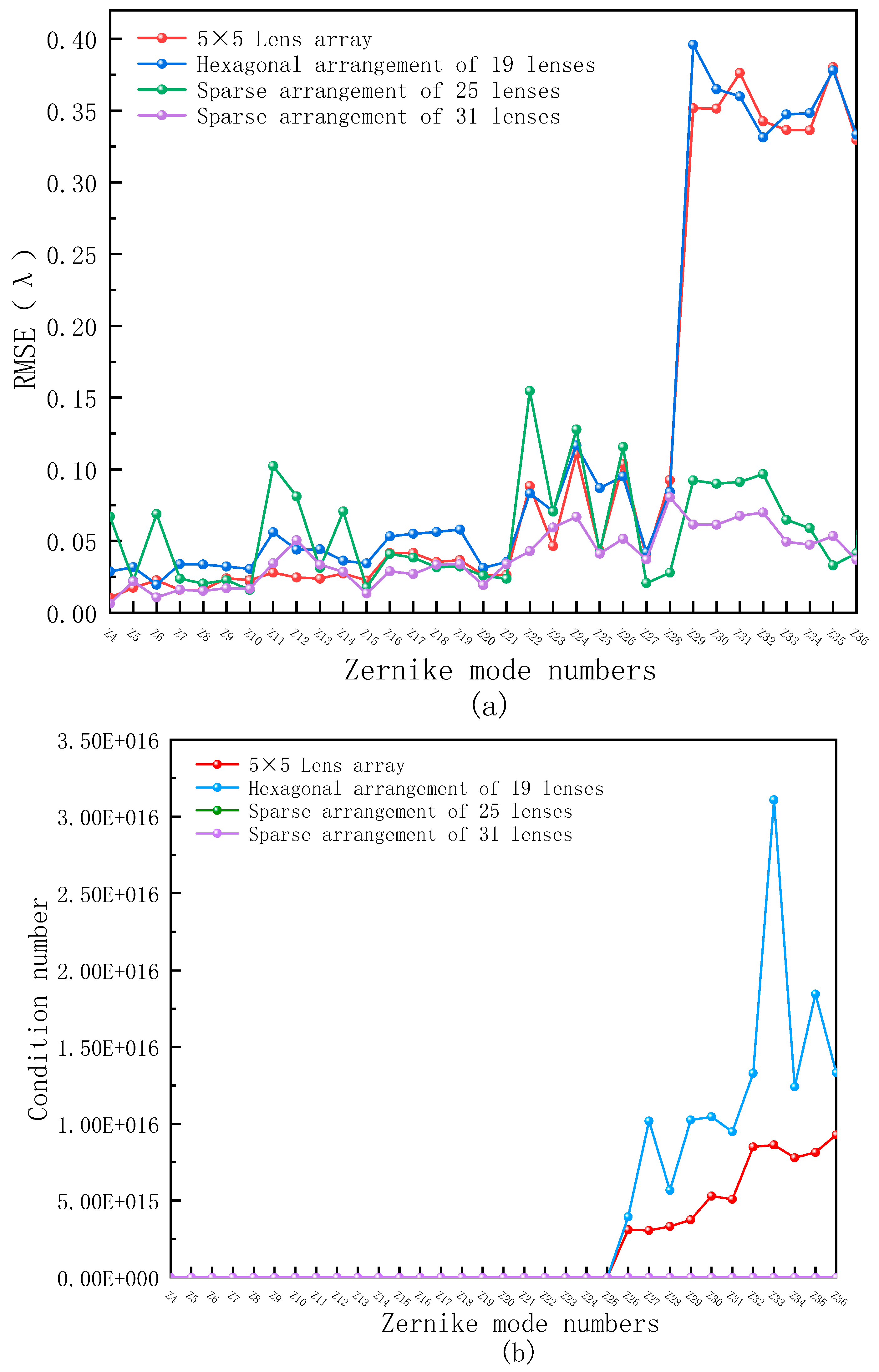
Figure 6.
Reconstruction results of turbulent wavefront aberrations by the examined sparse arrangements.
Figure 6.
Reconstruction results of turbulent wavefront aberrations by the examined sparse arrangements.
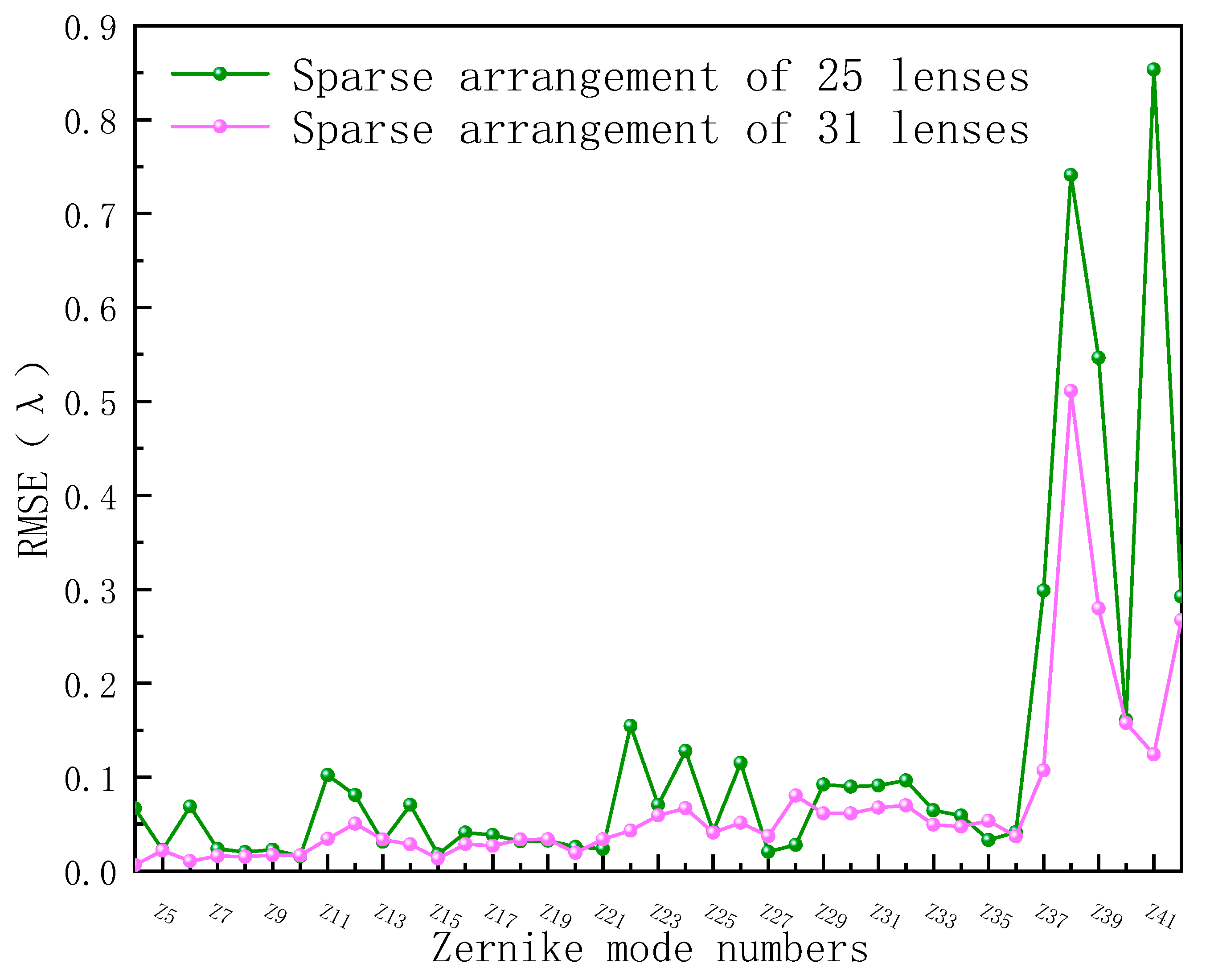
Figure 7.
RMS values of 50 turbulent wavefronts.
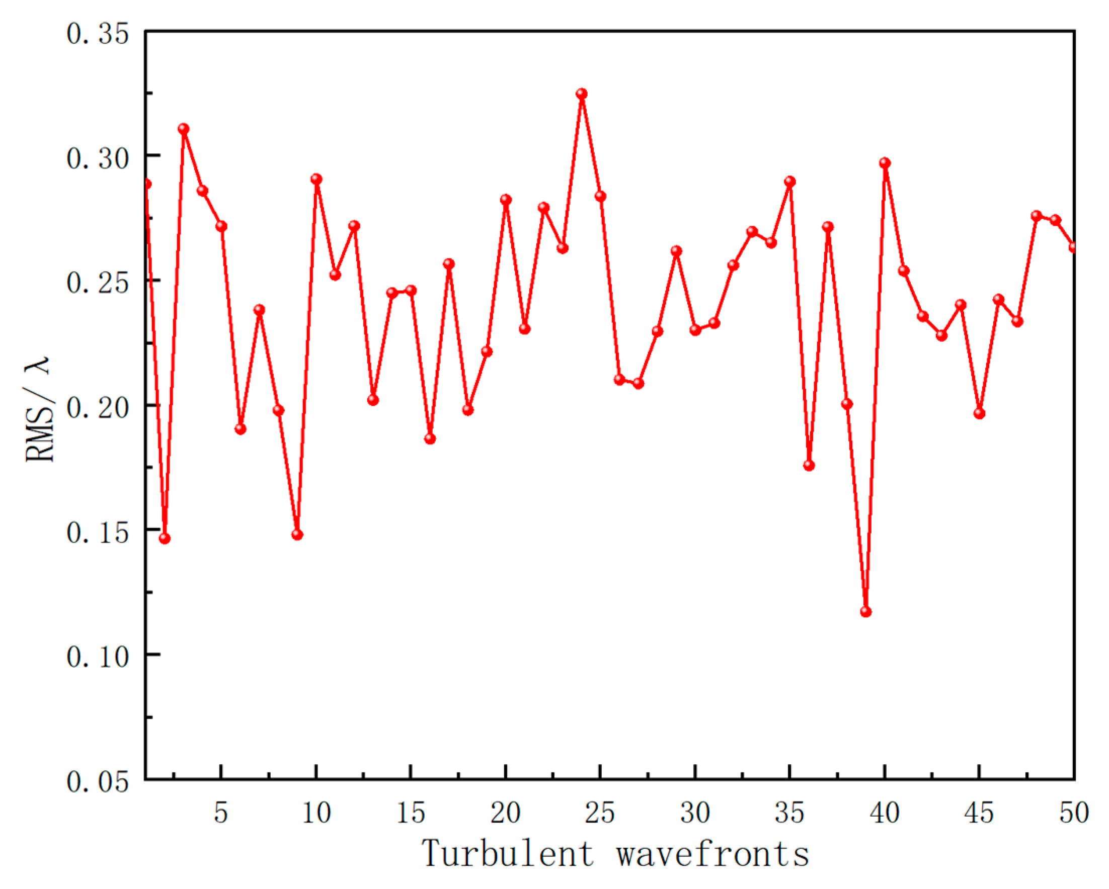
Figure 8.
Turbulent wavefront reconstruction.

Figure 9.
The turbulent wavefront reconstruction accuracy of the different lens arrangements. (a) A 28-order turbulent wavefront, (b) a 21-order turbulent wavefront.
Figure 9.
The turbulent wavefront reconstruction accuracy of the different lens arrangements. (a) A 28-order turbulent wavefront, (b) a 21-order turbulent wavefront.

Table 1.
System input parameters.
| Parameter | Description |
|---|---|
| Pixel size/μm | 4.5 |
| Beam wavelength/nm | 1064 |
| Lens size/mm | 25.4 |
| Lens spacing/mm | 6.35 |
| Duty factor | 0.8 |
| Lens focal length/mm | 1200 |
Table 2.
The statistical values of the recovery accuracy for the different orders of single aberrations of the four lens array arrangements.
Table 2.
The statistical values of the recovery accuracy for the different orders of single aberrations of the four lens array arrangements.
| Quantity | Mean | Standard Deviation | Variance | |
|---|---|---|---|---|
| 5 × 5 Lens array | 25 | 0.03944 | 0.02821 | 7.96036 × 10⁻⁴ |
| Hexagonal arrangement of 19 lenses | 25 | 0.05175 | 0.02475 | 6.12562 × 10⁻⁴ |
| 25 Units sparsely arranged | 25 | 0.05184 | 0.03849 | 0.00148 |
| 31 Units sparsely arranged | 25 | 0.03282 | 0.01831 | 3.35307 × 10⁻⁴ |
Disclaimer/Publisher’s Note: The statements, opinions and data contained in all publications are solely those of the individual author(s) and contributor(s) and not of MDPI and/or the editor(s). MDPI and/or the editor(s) disclaim responsibility for any injury to people or property resulting from any ideas, methods, instructions or products referred to in the content. |
© 2024 by the authors. Licensee MDPI, Basel, Switzerland. This article is an open access article distributed under the terms and conditions of the Creative Commons Attribution (CC BY) license (https://creativecommons.org/licenses/by/4.0/).
Share and Cite
MDPI and ACS Style
Wang, G.; Qin, L.; Li, Y.; Cheng, Y.; Jing, X.; Chen, G.; Hou, Z. Simulation Analysis of an Atmospheric Turbulence Wavefront Measurement System. Photonics 2024, 11, 383. https://doi.org/10.3390/photonics11040383
AMA Style
Wang G, Qin L, Li Y, Cheng Y, Jing X, Chen G, Hou Z. Simulation Analysis of an Atmospheric Turbulence Wavefront Measurement System. Photonics. 2024; 11(4):383. https://doi.org/10.3390/photonics11040383
Chicago/Turabian StyleWang, Gangyu, Laian Qin, Yang Li, Yilun Cheng, Xu Jing, Gongye Chen, and Zaihong Hou. 2024. "Simulation Analysis of an Atmospheric Turbulence Wavefront Measurement System" Photonics 11, no. 4: 383. https://doi.org/10.3390/photonics11040383
Note that from the first issue of 2016, this journal uses article numbers instead of page numbers. See further details here.