A Deep Learning-Based Preprocessing Method for Single Interferometric Fringe Patterns

Shaanxi Province Key Laboratory of Thin Films Technology and Optical Test, Xi’an Technological University, Xi’an 710021, China
*
Author to whom correspondence should be addressed.
Photonics 2024, 11(3), 226; https://doi.org/10.3390/photonics11030226
Submission received: 5 January 2024
/
Revised: 26 February 2024
/
Accepted: 27 February 2024
/
Published: 29 February 2024
(This article belongs to the Special Issue Optical Imaging and Measurements)
Abstract
:A novel preprocessing method based on a modified U-NET is proposed for single interference fringes. The framework is constructed by introducing spatial attention and channel attention modules to optimize performance. In this process, interferometric fringe maps with an added background intensity, fringe amplitude, and ambient noise are used as the input to the network, which outputs fringe maps in an ideal state. Simulated and experimental results demonstrated that this technique can preprocess single interference fringes in ~1 microsecond. The quality of the results was further evaluated using the root mean square error, peak signal-to-noise ratio, structural similarity, and equivalent number of views. The proposed method outperformed U-NET, U-NET++, and other conventional algorithms as measured by each of these metrics. In addition, the model produced high-quality normalized fringes by combining objective data with visual effects, significantly improving the accuracy of the phase solutions for single interference fringes.
1. Introduction
Interferometry is an active area of research in which the processing of fringe maps is essential to recovering hidden three-dimensional surface shapes [1]. However, when phase demodulation is performed on single interference fringes, the background intensity, fringe amplitude, and ambient noise present at the time of data acquisition can affect the contrast of fringes and ultimately the accuracy of phase reconstruction. As such, a variety of single interferometry techniques have been introduced in recent years to address this issue [2,3,4,5,6]. These methods require only one interferometric fringe map for phase extraction and are primarily applied to dynamic measurements requiring high real-time performance. This includes the Fourier transform [2,3], regularized phase tracking [4], and Hilbert transform methods [5,6]. In the case of single interference fringes, a lack of contrast can cause serious distortions in the resulting phase distribution. As such, filtering ambient noise, normalizing the background intensity and the fringe amplitude are necessary preprocessing steps when reconstructing the phase of single interference fringe data [7,8,9].
These techniques have been implemented in several previous studies. For example, Quiroga [10] proposed an orthogonal projection algorithm used for background suppression and modulation normalization. Ochoa [11] developed a process for normalizing and denoising fringe maps using directional derivatives. Bernini [12] proposed a technique based on 2D empirical modal decomposition and Hilbert transforms for the normalization of striped images. Tien [13] developed a fringe normalization algorithm using Zernike polynomial fitting to eliminate unwanted intensity in interferograms, suppressing background pixels and high frequency noise while improving contrast through normalization. Sharma [14] introduced a fringe normalization and denoising process based on Kalman filtering to fit background and modulation terms using a raster scan. Leijie [15] proposed a fringe map orthogonalization method based on a series of GANs, which achieved phase demodulation of single interference fringes with high accuracy.
In response to the above analysis, this paper proposes a preprocessing method for single interference fringes, in order to quickly and easily realize the denoising and normalization of single interferometric fringe patterns, and to lay the foundation for the subsequent phase solution of single interferometric fringe patterns, in which denoising and normalization are achieved using an improved U-NET framework. The algorithm was trained by first determining the form of the background and fringe structures. Gaussian noise and corresponding interference fringes were then added under ideal conditions to establish sample pairs. Four different evaluation metrics, including root the mean square error (RMSE), peak signal-to-noise ratio (PSNR), structural similarity index measure (SSIM), and equivalent number of looks (ENL) were utilized to verify the feasibility of this process. Finally, the proposed method was further assessed using a series of experimentally acquired single interference fringes.
2. Method
2.1. Interference Fringe Model
Interference in fringes can be expressed mathematically as:
where is the background intensity in a fringe map, is the fringe amplitude, is a phase term associated with a measured physical quantity, and is additional noise. Normalizing the background and fringe amplitude, while filtering additional noise, allows for the interference (after preprocessing) to be represented as
The modulated and background intensity can be determined from a comparative analysis to be in the form of a Gaussian function given by:
where is a spatial coordinate, is a center point coordinate, is the magnitude, and denote the variance.
2.2. The DN-U-NET Network Model
U-NETs [16] are improved fully convolutional neural networks designed to solve problems in medical image segmentation. They exhibit several robust properties that have led to an increasing number of applications in a wide variety of tasks. The purpose of this paper is to achieve pre-processing, in the form of denoising and normalization, for single interferometric fringes using an improved U-NET neural network. The proposed model is thus termed a denoising and normalization U-NET (DN-U-NET).
This process involved the use of an attention mechanism [17], a technique that emphasizes key information by assigning different weights to individual features to improve model accuracy. Attention mechanisms have been widely used in various deep learning tasks, such as computer vision and natural language processing. The convolutional block attention module (CBAM [18]) divides this attention step into two separate components, a channel attention module and a spatial attention module, which not only preserves parameters and computational power, but also facilitates integration into existing network architectures as a plug-and-play module. This inclusion typically improves extraction accuracy and network generalizability. The bottleneck attention module (BAM [19]) was developed by the same group that proposed CBAM. While these frameworks are similar, the CBAM module can be described as a series connection of channel attention and spatial attention modules. In contrast, the BAM module can be viewed as a parallel connection (see Figure 1 and Figure 2). The DN-U-NET network structure is shown in Figure 3, where the input consists of interference fringes with a certain background intensity, fringe amplitude, and added ambient noise. The output includes corresponding interference fringes in an ideal state.
2.3. Dataset and Environment Configuration
The included dataset consists of two parts: interferometric fringes with an added background intensity (i.e., fringe amplitude and ambient noise), and the corresponding fringes in an ideal state. The Zernike polynomials are a set of complete orthogonal bases in the unit-circle domain constructed by the Dutch scientist F. Zernike in 1934 during his research on phase contrast microscopy, and their use as a basis function for phase fitting can correspond well with the classical phase differences of optical systems and provide the necessary conditions for subsequent studies. Random phases were generated using Zernike polynomials as follows:
where represents Zernike polynomial coefficients (). In the simulation, in order to be able to post-simulate phase data that are closer to the practical application, the values of the Zernike polynomial coefficients are kept consistent with those of the experimental data from the Zygo interferometer. These coefficients were generated using a random function, with a range of values shown in Table 1.
A total of 12,000 pairs of input and ideal stripe maps were generated using a simulation, with sizes of 256 × 256 pixels. These images were input to the network and used for training, with a 5:1 ratio of samples in the training and test sets. The TensorFlow framework was implemented using Python on a PC with an Intel(R) Xeon(R) Gold 5218R CPU @ 2.10 GHz. Calculations were accelerated using an NVIDIA GeForce RTX 3080. Weighting parameters were optimized using the Adam optimizer, with a learning rate set to a fixed value of 0.0001. A total of 500 iterations were performed, with a training time of ~40 h required to identify ideal weights. The corresponding loss function, minimized as part of the training process, could be expressed mathematically as:
where is a fringe map generated by the network, is a truth value, and is the minimum number of input data batches.
2.4. Evaluation Indicators
Four numerical metrics were selected to evaluate the results and quantify deviations from true values, both before and after denoising and normalization. This included the root mean square error (RMSE), peak signal-to-noise ratio (PSNR), structural similarity index measure (SSIM), and equivalent number of looks (ENL).
The RMSE represents the extent to which measured data deviate from true data, with smaller values indicating a higher accuracy. This term can be expressed mathematically as
where and denote the width and height of a fringe map, respectively, represents preprocessed data before or after, and are true value data.
The PSNR captures differences between corresponding pixels in a preprocessed image and a true value image, represented as
where 2n−1 represents the maximum gray value of a pixel in an image (n = 8). The MSE can be expressed as
The SSIM is used to evaluate the similarity of two images and is given by
where are two localized windows of size W × W in the true value data and the data before and after preprocessing, respectively. The terms are the averages of pixel gray values in the two windows, respectively, while is the variance and C1 and C2, respectively, describe the covariance of the two windows.
ENL provides a measure of the smoothness of a homogeneous region and can be expressed as
where denote the mean and standard deviation of pixel values in an image, respectively.
3. Simulation and Analysis
Six different sets of fringes were processed using DN-U-NET, as shown in Figure 4. Specifically, Figure 4a shows fringe samples in an ideal state, in which the background intensity and fringe amplitude are constant. Figure 4b shows fringes before processing, in which the background intensity and fringe amplitude (in the form of a Gaussian function) were added along with Gaussian noise. Figure 4c displays corresponding results after processing with DN-U-NET. Visual inspection suggests that the processed fringes exhibit improved contrast while noise was suppressed significantly, producing results that are more similar to the ideal fringes.
The proposed DN-U-NET was compared with existing algorithms, including a U-NET, UNET++ [20], R2-UNET [21], Attention_U-NET [22], and U-NET3+ [23]. The training of each neural network model was conducted using the same dataset and methodology as that of the proposed network. Figure 5 shows a series of interference fringes in an ideal state, with added background intensity, corresponding fringe amplitude, and ambient noise. A comparison of denoising and normalization results is also provided for several models. Visual inspection suggests that several of these techniques significantly enhanced fringe contrast and provided significant suppression of noise. The metrics described above were used to quantify the effectiveness of fringe denoising and normalization, for comparison with conventional algorithms. Table 2 provides a comparative analysis of interference fringe denoising and normalization results from different models, with bold font denoting the best (highest or lowest) values. It is evident that several algorithms achieved significant improvements across each evaluation index compared with the original noisy image. The processing times of several different networks for a single interference fringe are all 1 microsecond. Notably, the proposed DN-U-NET produced improvements of 0.2986 (RMSE), 0.5712 dB (PSNR), and 0.0009 (SSIM) compared with the standard U-NET algorithm. A global ENL evaluation further demonstrated an increase of 0.0071. The proposed DN-U-NET network performs the best for all four evaluation metrics. For the indicator of the RMSE, comparing with the before processing, it is improved from 96.0986 to 4.3928, which is a very obvious improvement. Comparing with U-NET++, it is improved from 5.0276 to 4.3928, which is an improvement of up to 12.6%, and in the indicator of PSNR, comparing with the before processing, it is improved from 8.4765 dB to 35.2760 dB, which is an improvement of 26.7998 dB, and comparing to U-NET++, from 34.1035 dB to 35.2760 dB, an improvement of 1.1725 dB.
The validity and stability of the proposed method were further verified through the addition of background intensity and fringe amplitude. These signals were added to the label fringes shown in Figure 5a and assumed the form of a Gaussian function and Gaussian noise with a mean of 0. Fringes with standard deviation levels of 0, 0.05, 0.07, 0.09, 0.12, and 0.15 are shown in Figure 6a–f, respectively. The DN-U-NET was also used to perform the pre-processing operations of denoising and normalization at varying noise intensities, as shown in Figure 6g–l. A visual inspection suggests that these processed interference fringes exhibit significantly improved contrast, as noise has been effectively suppressed. These results were also quantitatively analyzed, as described below. Specifically, Table 3 provides a comparative analysis of the denoising and normalization effects produced by the DN-U-NET. It is evident that the processed images have improved significantly, as measured by RMSE, PSNR, SSIM, and ENL. Notably, at a noise level of 0.15, these evaluation metrics have a decreased but remain at a desirable value. This outcome provides more evidence for the effectiveness and stability of the proposed technique for denoising and normalizing interference fringes, even at high noise levels.
The effectiveness of the proposed processing method was further verified by solving for the phase of single interference fringes using a technique proposed in the literature [24]. The accuracy of the phase before and after this single processing step was then compared to provide an evaluation of performance. A single interference fringe in an ideal state is shown in Figure 7a, while Figure 7b shows a corresponding label phase with PV and RMS values of 0.1334 λ and 0.0289 λ, respectively. Figure 7c shows a single fringe before processing, while Figure 7d shows the corresponding phase after processing, with PV and RMS values of 0.0448 λ and 0.0105 λ, respectively. Figure 7e shows the error between the solved phase acquired before processing and the label phase, with residual PV and RMS values of 0.1174 λ and 0.0254 λ, respectively. Figure 7f displays a single interference fringe after processing, with Figure 7g providing the corresponding phase after processing, with PV and RMS values of 0950 λ and 0.0221 λ, respectively. Figure 7h provides the phase error between the processed phase and label phase, with residual PV and RMS values of 0.0566 λ and 0.0111 λ, respectively. A comparison of the reconstructed phase accuracy before and after processing demonstrated that residual PV improved from 0.1174 λ to 0.0566 λ, while residual RMS improved from 0.0254 λ to 0.0111 λ. Simulated results also indicated the method proposed in this paper could improve fringe contrast while suppressing fringe noise, significantly improving the accuracy of single interference fringe phase, which furthered validated the effectiveness and necessity of the technique proposed in this paper.
4. Experimental Analysis
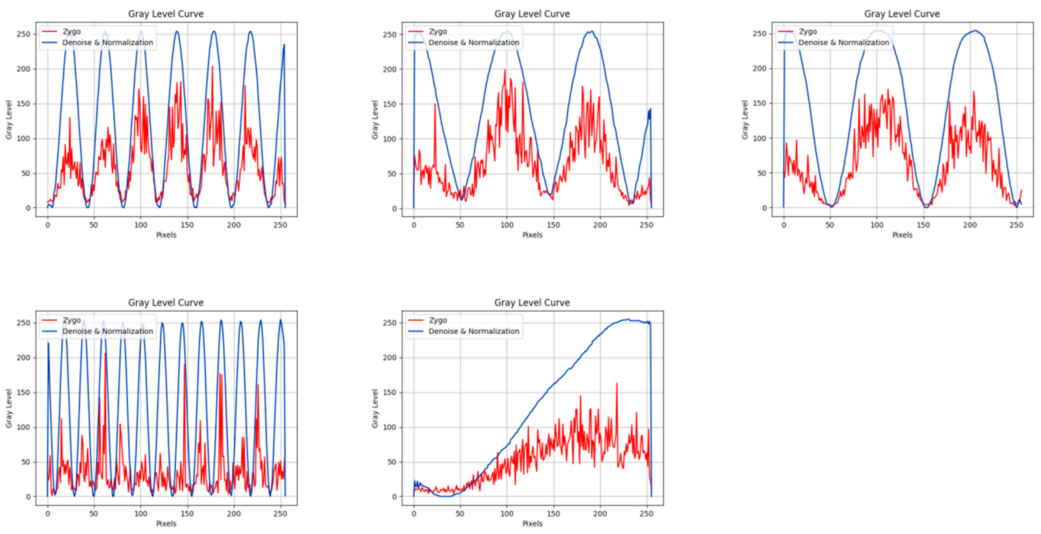
In addition to the use of simulated fringes, DN-U-NET performance was evaluated with a series of experimentally collected fringe maps, as shown in Figure 8a. The original interference fringe pattern was collected using a ZYGO-Verifire PE Fischer-type phase-shifting interferometer, using different networks, the Zygo original interference fringes are processed, respectively, and the processing results are shown in Figure 8. Through visual observation, several models can significantly enhance their stripe contrast and significantly suppress noise when processing the Zygo original interference fringe. In order to compare the effect before and after processing, the results of several different models are compared with the gray scale distribution curve of the 128th line before and after processing, and the comparison results are shown in Figure 9. In addition, the processing results of the U-NET network are compared with the processing results of the DN-U-NET proposed in this paper, and the comparison results are shown in Figure 10, which shows that the gray level distribution of the interference fringes after the processing of the model proposed in this paper is smoother and more average.
The original interference fringe pattern was collected using a ZYGO-Verifire PE Fischer-type phase-shifting interferometer with different plane mirrors serving as the measurement sample. It is evident that the contrast is poor and obvious noise is present. The fringes shown in Figure 11a were then processed using the proposed technique, the results of which are shown in Figure 11b. A visual inspection suggests the contrast has been enhanced while the ambient noise has been suppressed significantly. Figure 12 provides a comparison of gray level distribution curves for the 128th line in the two fringe maps shown in Figure 11a,b, which are evidently smoother after preprocessing. Notably, this process requires only a single microsecond (10−6 s) of runtime for each interference fringe.
Figure 13b shows the original interference fringe acquired with the interferometer, while Figure 13e displays the interference fringe after processing using the method proposed in this paper. The measured phase distribution was then compared with the phase acquired using a four-step phase-shifting technique, which served as the reference phase (see Figure 13a). This process produced PV and RMS values of 0.1381 λ and 0.0300 λ, respectively. Figure 13c shows the corresponding phase distribution before processing, with PV and RMS values of 0.0670 λ and 0.0110 λ, respectively. Figure 13e displays the phase error between the solved phase (before processing) and the reference phase, with residual PV and RMS values of 0.1200 λ and 0.0267 λ, respectively. Figure 13f shows the corresponding phase solved after processing, with a PV and RMS of 0.1110 λ and 0.0241 λ, respectively. Figure 13g shows the error between the solved phase (after processing) and the reference phase, with a residual PV and RMS of 0.0856 λ and 0.0121 λ, respectively. A comparison of the reconstructed phase accuracy before and after processing indicated that residual PV improved from 0.1200λ to 0.0856λ, while residual RMS improved from 0.0300 λ to 0.0121 λ. These experimental results also demonstrate that the method proposed in this paper can significantly improve phase reconstruction accuracy while improving the fringe contrast.
5. Conclusions
In this study, a neural network-based preprocessing model (DN-U-NET) was proposed for single interference fringes. This technique was applied to determine the form of fringe amplitude and background intensity structures, as well as generate fringe maps with an added background intensity, additional amplitude, and ambient noise. The simulated interferometric fringes were generated in an ideal state using Zernike polynomials. The network was then constructed, trained, and tested using the synthetic dataset. Experimental results demonstrated that this technique can efficiently achieve denoising and normalization of single interference fringes, significantly improving contrast while producing high-quality normalized fringes. The reconstructed phase accuracy was also improved for single interference fringes.
Author Contributions
Conceptualization, X.Z. and A.T; methodology, X.Z., D.Z., B.L. and A.T.; validation, D.Z.; formal analysis, X.Z.; investigation, Y.H.; data curation, X.Z., B.L. and H.W.; writing—original draft preparation, X.Z. and D.Z.; writing—review and editing, X.Z. and Y.H.; supervision, Y.H. All authors have read and agreed to the published version of the manuscript.
Funding
This research was funded by Shaanxi Provincial Science and Technology (grant numbers 2024GX-YBXM-234).
Institutional Review Board Statement
Not applicable.
Informed Consent Statement
Not applicable.
Data Availability Statement
Data underlying the results presented in this paper are not publicly available at this time but may be obtained from the authors upon reasonable request.
Acknowledgments
We thank LetPub for linguistic assistance and a pre-submission expert review.
Conflicts of Interest
The authors declare no conflict of interest.
References
- Leach, R.K.; Senin, N.; Feng, X.; Stavroulakis, P.; Su, R.; Syam, W.P.; Widjanarko, T. Information-rich metrology: Changing the game. Commer. Micro Manuf. 2017, 8, 33–39. [Google Scholar]
- Servin, M.; Cuevas, F.J. A novel technique for spatial phase-shifting interferometry. J. Mod. Opt. 1995, 42, 1853–1862. [Google Scholar] [CrossRef]
- Servin, M.; Estrada, J.C.; Medina, O. Fourier transform demodulation of pixelated phase-masked interferograms. Opt. Express 2010, 18, 16090–16095. [Google Scholar] [CrossRef] [PubMed]
- Li, J.P.; Song, L.; Chen, L.; Li, B.; Han, Z.G.; Gu, C.F. Quadratic polar coordinate transform technique for the demodulation of circular carrier interferogram. Opt. Commun. 2015, 336, 166–172. [Google Scholar] [CrossRef]
- Servin, M.; Marroquin, J.L.; Quiroga, J.A. Regularized quadrature and phase tracking from a single closed-fringe interferogram. J. Opt. Soc. Am. A 2004, 21, 411–419. [Google Scholar] [CrossRef] [PubMed]
- Kai, L.; Kemao, Q. Improved generalized regularized phase tracker for demodulation of a single fringe pattern. Opt. Express 2013, 21, 24385–24397. [Google Scholar] [CrossRef] [PubMed]
- Quiroga, J.A.; Servin, M. Isotropic n-dimensional fringe pattern normalization. Opt. Commun. 2003, 224, 221–227. [Google Scholar] [CrossRef]
- Servin, M.; Marroquin, J.L.; Cuevas, F.J. Fringe-follower regularized phase tracker for demodulation of closed-fringe interferograms. J. Opt. Soc. Am. A 2001, 18, 689–695. [Google Scholar] [CrossRef]
- Rivera, M. Robust phase demodulation of interferograms with open or closed fringes. J. Opt. Soc. Am. A 2005, 22, 1170–1175. [Google Scholar] [CrossRef] [PubMed]
- Quiroga, J.A.; Gómez-Pedrero, J.A.; García-Botella, Á. Algorithm for fringe pattern normalization. Opt. Commun. 2001, 197, 43–51. [Google Scholar] [CrossRef]
- Ochoa, N.A.; Silva-Moreno, A.A. Normalization and noise-reduction algorithm for fringe patterns. Opt. Commun. 2007, 270, 161–168. [Google Scholar] [CrossRef]
- Bernini, M.B.; Federico, A.; Kaufmann, G.H. Normalization of fringe patterns using the bidimensional empirical mode decomposition and the Hilbert transform. Appl. Opt. 2009, 48, 6862–6869. [Google Scholar] [CrossRef] [PubMed]
- Tien, C.L.; Jyu, S.S.; Yang, H.M. A method for fringe normalization by Zernike polynomial. Opt. Rev. 2009, 16, 173–175. [Google Scholar] [CrossRef]
- Sharma, S.; Kulkarni, R.; Ajithaprasad, S.; Gannavarpu, R. Fringe pattern normalization algorithm using Kalman filter. Results Opt. 2021, 5, 100152. [Google Scholar] [CrossRef]
- Feng, L.; Du, H.; Zhang, G.; Li, Y.; Han, J. Fringe Pattern Orthogonalization Method by Generative Adversarial Nets. Acta Photonica Sin. 2023, 52, 0112003. [Google Scholar]
- Ronneberger, O.; Fischer, P.; Brox, T. U-net: Convolutional networks for biomedical image segmentation. In Proceedings of the Medical Image Computing and Computer-Assisted Intervention–MICCAI 2015: 18th International Conference, Munich, Germany, 5–9 October 2015; Proceedings, Part III 18. Springer International Publishing: Cham, Switzerland, 2015; pp. 234–241. [Google Scholar]
- Vaswani, A.; Shazeer, N.; Parmar, N.; Uszkoreit, J.; Jones, L.; Gomez, A.N.; Kaiser, Ł.; Polosukhin, I. Attention is all you need. arXiv 2017, arXiv:1706.03762. [Google Scholar]
- Woo, S.; Park, J.; Lee, J.Y.; Kweon, I.S. Cbam: Convolutional block attention module. In Proceedings of the European Conference on Computer Vision (ECCV), Munich, Germany, 8–14 September 2018; pp. 3–19. [Google Scholar]
- Park, J.; Woo, S.; Lee, J.Y.; Kweon, I.S. BAM: Bottleneck Attention Module. In Proceedings of the British Machine Vision Conference (BMVC). British Machine Vision Association (BMVA), Newcastle, UK, 3–6 September 2018. [Google Scholar]
- Zhou, Z.; Siddiquee, M.M.R.; Tajbakhsh, N.; Liang, J. Unet++: A nested u-net architecture for medical image segmentation. In Deep Learning in Medical Image Analysis and Multimodal Learning for Clinical Decision Support: 4th International Workshop, DLMIA 2018, and 8th International Workshop, ML-CDS 2018, Held in Conjunction with MICCAI 2018, Granada, Spain, 20 September 2018, Proceedings 4; Springer International Publishing: Cham, Switzerland, 2018; pp. 3–11. [Google Scholar]
- Alom, Z.; Yakopcic, C.; Hasan, M.; Taha, T.M.; Asari, V.K. Recurrent residual U-Net for medical image segmentation. J. Med. Imaging 2019, 6, 014006. [Google Scholar] [CrossRef] [PubMed]
- Abraham, N.; Khan, N.M. A novel focal tversky loss function with improved attention u-net for lesion segmentation. In Proceedings of the 2019 IEEE 16th International Symposium on Biomedical Imaging (ISBI 2019), Venice, Italy, 8–11 April 2019; pp. 683–687. [Google Scholar]
- Huang, H.; Lin, L.; Tong, R.; Hu, H.; Zhang, Q.; Iwamoto, Y.; Han, X.; Chen, Y.W.; Wu, J. Unet 3+: A full-scale connected unet for medical image segmentation. In Proceedings of the ICASSP 2020-2020 IEEE International Conference on Acoustics, Speech and Signal Processing (ICASSP), Barcelona, Spain, 4–8 May 2020; pp. 1055–1059. [Google Scholar]
- Liu, X.; Yang, Z.; Dou, J.; Liu, Z. Fast demodulation of single-shot interferogram via convolutional neural network. Opt. Commun. 2021, 487, 126813. [Google Scholar] [CrossRef]
Figure 1.
A diagram of the CBAM module.

Figure 2.
A diagram of the BAM module.

Figure 3.
A diagram of the DN-U-Net network architecture.

Figure 4.
A comparison of pre-processing effects after denoising and normalization. Included images represent (a) labels and samples both (b) before processing and (c) after processing.
Figure 4.
A comparison of pre-processing effects after denoising and normalization. Included images represent (a) labels and samples both (b) before processing and (c) after processing.

Figure 5.
A comparison of pre-processing effects after denoising and normalization using different network models.
Figure 5.
A comparison of pre-processing effects after denoising and normalization using different network models.

Figure 6.
A comparison of fringe patterns before and after processing at different noise levels. (a) Before processing (noise level = 0). (b) Before processing (noise level = 0.05). (c) Before processing (noise level = 0.07). (d) Before processing (noise level = 0.09). (e) Before processing (noise level = 0.12). (f) Before processing (noise level = 0.15). (g) After processing (noise level = 0). (h) After processing (noise level = 0.05). (i) After processing (noise level = 0.07). (j) After processing (noise level = 0.09). (k) After processing (noise level = 0.12). (l) After processing (noise level = 0.15).

Figure 7.
A comparison of the reconstructed phase before and after processing. (a) Label; (b) label phase; (c) before processing; (d) phase distribution before processing; (e) reconstructed error before processing; (f) after processing; (g) phase distribution after processing; (h) reconstructed error after processing.

Figure 8.
Comparison of the effects of different network models in dealing with the Zygo original interference fringe denoising and normalized preprocessing.
Figure 8.
Comparison of the effects of different network models in dealing with the Zygo original interference fringe denoising and normalized preprocessing.

Figure 9.
Comparison of gray scale distribution curves at row 128 before and after the processing of different network models.
Figure 9.
Comparison of gray scale distribution curves at row 128 before and after the processing of different network models.

Figure 10.
Comparison of the DN-U-NET and U-NET preprocessing results.

Figure 11.
(a) Interference fringes collected experimentally using a Zygo interferometer. (b) The processed image.
Figure 11.
(a) Interference fringes collected experimentally using a Zygo interferometer. (b) The processed image.

Figure 12.
The 128th gray distribution curve before and after processing.

Figure 13.
A comparison of the reconstructed phase before and after processing. (a) label phase; (b) before processing; (c) phase distribution before processing; (d) reconstructed error before processing; (e) after processing; (f) phase distribution after processing; (g) reconstructed error after processing.


Table 1.
The range of Zernike polynomial data.
| Zernike Coefficient | a1 | a2–a3 | a4–a6 | a7–a36 |
| Value Range/λ | 0 | [−3, 3] | [−0.1, 0.1] | [−0.01, 0.01] |
Table 2.
A comparison of the denoising and normalization effects produced by different network models.
Table 2.
A comparison of the denoising and normalization effects produced by different network models.
| Method | RMSE | PSNR | SSIM | ENL | |||||
|---|---|---|---|---|---|---|---|---|---|
| Before | After | Before | After | Before | After | Label | Before | After | |
| U-NET | 96.0986 | 4.6914 | 8.4765 | 34.7048 | 0.3857 | 0.9888 | 1.0845 | 0.7979 | 1.0728 |
| U-NET++ | 5.0276 | 34.1035 | 0.9869 | 1.0783 | |||||
| R2_U-NET | 4.5779 | 34.9174 | 0.9895 | 1.0780 | |||||
| Attention_U-NET | 4.5777 | 34.9178 | 0.9895 | 1.0779 | |||||
| U-NET3+ | 4.9441 | 34.2490 | 0.9873 | 1.0789 | |||||
| DN-U-NET | 4.3928 | 35.2760 | 0.9897 | 1.0799 | |||||
Table 3.
A quantitative comparison of denoising and normalization effects at varying noise levels.
| Noise Level | RMSE | PSNR | SSIM | ENL | |||||
|---|---|---|---|---|---|---|---|---|---|
| Before | After | Before | After | Before | After | Label | Before | After | |
| 0 | 94.6761 | 3.7286 | 8.6060 | 36.6999 | 0.4665 | 0.9880 | 1.0845 | 0.8186 | 1.0670 |
| 0.05 | 95.1219 | 3.7145 | 8.5652 | 36.7329 | 0.4459 | 0.9907 | 0.8361 | 1.0701 | |
| 0.07 | 95.4267 | 3.0072 | 8.5374 | 38.5675 | 0.4210 | 0.9935 | 0.8209 | 1.0735 | |
| 0.09 | 95.8054 | 4.1439 | 8.5030 | 35.7826 | 0.3968 | 0.9895 | 0.8059 | 1.0785 | |
| 0.12 | 96.4116 | 3.8796 | 8.4482 | 36.3551 | 0.3678 | 0.9910 | 0.7723 | 1.0866 | |
| 0.15 | 96.9670 | 6.2108 | 8.3983 | 32.2678 | 0.3428 | 0.9800 | 0.7351 | 1.1135 | |
Disclaimer/Publisher’s Note: The statements, opinions and data contained in all publications are solely those of the individual author(s) and contributor(s) and not of MDPI and/or the editor(s). MDPI and/or the editor(s) disclaim responsibility for any injury to people or property resulting from any ideas, methods, instructions or products referred to in the content. |
© 2024 by the authors. Licensee MDPI, Basel, Switzerland. This article is an open access article distributed under the terms and conditions of the Creative Commons Attribution (CC BY) license (https://creativecommons.org/licenses/by/4.0/).
Share and Cite
MDPI and ACS Style
Zhu, X.; Zhang, D.; Hao, Y.; Liu, B.; Wang, H.; Tian, A. A Deep Learning-Based Preprocessing Method for Single Interferometric Fringe Patterns. Photonics 2024, 11, 226. https://doi.org/10.3390/photonics11030226
AMA Style
Zhu X, Zhang D, Hao Y, Liu B, Wang H, Tian A. A Deep Learning-Based Preprocessing Method for Single Interferometric Fringe Patterns. Photonics. 2024; 11(3):226. https://doi.org/10.3390/photonics11030226
Chicago/Turabian StyleZhu, Xueliang, Di Zhang, Yilei Hao, Bingcai Liu, Hongjun Wang, and Ailing Tian. 2024. "A Deep Learning-Based Preprocessing Method for Single Interferometric Fringe Patterns" Photonics 11, no. 3: 226. https://doi.org/10.3390/photonics11030226
Note that from the first issue of 2016, this journal uses article numbers instead of page numbers. See further details here.