HoloDiffusion: Sparse Digital Holographic Reconstruction via Diffusion Modeling

Abstract

In digital holography, reconstructed image quality can be primarily limited due to the inability of a single small aperture sensor to cover the entire field of a hologram. The use of multi-sensor arrays in synthetic aperture digital holographic imaging technology contributes to overcoming the limitations of sensor coverage by expanding the area for detection. However, imaging accuracy is affected by the gap size between sensors and the resolution of sensors, especially when dealing with a limited number of sensors. An image reconstruction method is proposed that combines physical constraint characteristics of the imaging object with a score-based diffusion model, aiming to enhance the imaging accuracy of digital holography technology with extremely sparse sensor arrays. Prior information of the sample is learned by the neural network in the diffusion model to obtain a score function, which alternately constrains the iterative reconstruction process with the underlying physical model. The results demonstrate that the structural similarity and peak signal-to-noise ratio of the reconstructed images using this method are higher than the traditional method, along with a strong generalization ability.

1. Introduction

Digital holography (DH) utilizes digital cameras instead of traditional optical recording materials to capture holograms and employs numerical methods to reconstruct both the amplitude and phase information of the light field emitted by objects [1,2,3]. It has gained significant prominence as a crucial scientific tool in a wide range of applications, including three-dimensional recognition [4,5], microscopic imaging [6,7], and surface feature extraction [8,9].

Nevertheless, there are still certain areas that require further improvement in DH. The quality of the reconstruction is often limited by the field of hologram (FOH). The complete information of a large FOH cannot be detected by a single small aperture sensor. The multiplexing method can enhance the representation of high-frequency information, which is available in either the frequency domain or the holographic domain [10,11]. The resolution of single-aperture DH can be enhanced through the self-extrapolation method [12,13]. However, the potential for improvement is restricted when employing smaller single-aperture sensors or capturing holograms in long-range imaging scenarios [14].

The synthetic aperture technique substantially broadens the detection area of high-order diffraction fringes [15,16]. As a prevalent technique for recovering complex amplitude light fields of targets, the Gechberg–Saxton (GS) [17] algorithm restored phase by alternating iterations between the spatial domain and holographic domain. Fienup et al. improved the GS method by adding a feedback process for fast convergence [18]. To expand the effective detection area within the holographic field, Huang et al. use multiple sparse aperture sensors, facilitating large-scale information acquisition. A self-restoration method for sparse aperture arrays (SRSAAs) [19] is then proposed, designed to incrementally recover the missing information within the gaps between sensors. Based on the GS method, SRSAAs offer acceptable image reconstruction quality, and they are sensitive to the selection of the initial conditions. Owing to inadequate extraction and utilization of prior information pertaining to the target of the light field distribution, there is an increased likelihood of falling into local optima. In addition, the quality of the reconstructed image is inherently constrained by the performance capabilities of the sensors.

Recently, a diffusion model [20] with strong generative capabilities has been proposed and has shown excellent performance in various generative modeling tasks, including medical image generation [21,22], image editing [23], and super-resolution imaging [24].

In order to achieve high-quality digital holographic imaging of an expansive FOH, the HoloDiffusion method is proposed by incorporating the diffusion model into the iterative digital holographic reconstruction. Prior information on the complex amplitude of the target light field is learned from the amplitude-phase image dataset via a diffusion model. The rotating iterations between the spatial domain and the holographic domain serve to complement each other’s information. The acquired prior information is utilized to bolster the reconstruction process. The distribution and energy constraints of objects are imposed on the spatial domain image to procure high-quality images.

The rest of the paper is structured as follows. The basis of DH, diffusion model and the details of the proposed HoloDiffusion are described in Section 2. Experimental results under various conditions are presented in Section 3. The discussion and conclusion are in Section 4 and Section 5, respectively.

2. Materials and Methods

2.1. Digital Holography

The hologram captured by the sensor can be depicted as follows:

$$I={\left|O(x_h,\hspace{0.33em}{y}_h,\hspace{0.33em}{z}_h)+R(x_h,\hspace{0.33em}{y}_h,\hspace{0.33em}{z}_h)\right|}^2$$

(1)

where $O(x_h,\hspace{0.33em}{y}_h,\hspace{0.33em}{z}_h)$ represents the object wave function and $R(x_h,\hspace{0.33em}{y}_h,\hspace{0.33em}{z}_h)$ signifies the reference wave function.

The transfer function of the object can be formulated as follows:

$$t(x_1,\hspace{0.33em}{y}_1,\hspace{0.33em}{z}_1)=(1-a(x_1,\hspace{0.33em}{y}_1,\hspace{0.33em}{z}_1))\exp (-i\phi (x_1,\hspace{0.33em}{y}_1,\hspace{0.33em}{z}_1))$$

(2)

where $a(x_1,\hspace{0.33em}{y}_1,\hspace{0.33em}{z}_1)$ delineates the attenuation of the incident wave and $\phi (x_1,\hspace{0.33em}{y}_1,\hspace{0.33em}{z}_1)$ represents the phase introduced by the object. The transmission function $t(x_1,\hspace{0.33em}{y}_1,\hspace{0.33em}{z}_1)$ can be expressed as $1+g(x_1,\hspace{0.33em}{y}_1,\hspace{0.33em}{z}_1)$, where $g(x_1,\hspace{0.33em}{y}_1,\hspace{0.33em}{z}_1)$ characterizes the presence of the object and ‘1’ is the transmittance in the absence of an object.

According to the forward propagation of Fresnel diffraction, the plane wave $U(x_1,\hspace{0.33em}{y}_1)$ will be modulated into the following form when passing through the object:

$$O(x_h,\hspace{0.33em}{y}_h,\hspace{0.33em}{z}_h)=-{\displaystyle \iint g(x_1,\hspace{0.33em}{y}_1,\hspace{0.33em}{z}_1)}\hspace{0.33em}U\frac{i\exp (ikd)}{\lambda d}d{x}_{1}d{y}_1$$

(3)

where $d=\sqrt{{(x_h-x_1)}^2+{(y_h-y_1)}^2+{(z_h-z_1)}^2}$ describes the distance between the object and the hologram. $\lambda$ is the wavelength and $k=2\pi /\lambda$ represents the wavenumber. The expression for the backpropagation formula is

$$t(x_1,\hspace{0.33em}{y}_1,\hspace{0.33em}{z}_1)=U^{*}{\displaystyle \iint h(x_h,\hspace{0.33em}{y}_h,\hspace{0.33em}{z}_h)}\frac{i\exp (-ikd)}{\lambda d}d{x}_{h}d{y}_h$$

(4)

where $U^{*}$ denotes the complex conjugation of U. $h(x_h,\hspace{0.33em}{y}_h,\hspace{0.33em}{z}_h)$ is the normalization of the hologram acquired when the reference wave directly illuminates the sensor without any object present. The reconstruction of images is limited by the field of hologram. While the sparse aperture array self-recovery method offers a partial solution, its lack of utilization of deep learning techniques results in suboptimal image reconstruction, which is especially evident in highly sparse sensor arrays. In pursuit of richer information and high-quality results, a method termed HoloDiffusion is introduced. This method tackles image reconstruction challenges within highly sparse sensor arrays through the application of diffusion models. Furthermore, this method employs a score-based generative model to estimate the prior distribution of both amplitude and phase images.

2.2. Score-Based Generative Model

As illustrated in Figure 1, the score-based diffusion model considers the continuous distribution of data points over time in accordance with the gradual evolution of the diffusion process. It progressively transforms the data points into random noise through forward stochastic differential equations (SDEs). This process is subsequently reversed, reconstructing the data from the noise that generated the sample. Hence, training a neural network is feasible in terms of estimating the gradient of the log data distribution (i.e., ${\nabla }_x\log p(x)$), enabling numerical solutions for inverse SDEs.

The diffusion process ${\{x(t)\}}_{t=0}^T$ is parameterized by the continuous time variable $t\in [0,\hspace{0.33em}T]$, where $x(0)~p_0$, $x(T)~p_T$, $p_0$ is the data distribution and $p_T$ is an unstructured prior distribution devoid of $p_0$ information, such as a Gaussian distribution with a fixed mean and variance. This diffusion process can be modeled as a solution for a forward SDE:

$$dx=f(x,t)dt+g(t)dw$$

(5)

where $w$ is the standard Wiener process, $f(x,t)$ is called the drift coefficient of $x(t)$, and $g(t)$ is the diffusion coefficient of $x(t)$.

Given that the reverse of the diffusion process is also a diffusion process [25], the solution for the reverse SDE can be formulated as follows:

$$dx=[f(x,t)-g{(t)}^2{\nabla }_x\log p_t(x)]dt+g(t)d\overline{w}$$

(6)

where $\overline{w}$ is the standard Wiener process with time ranging from $T$ to 0, and $dt$ is an infinitesimal negative step. Once the score ${\nabla }_x\log p_t(x)$ for each marginal distribution is known for all $t$, the reverse diffusion process can be derived from the above equation and then simulated in order to sample from $p_0$.

Different SDEs can be constructed by selecting various functions: $f(x,t)$ and $g(t)$. To mitigate the variance explosion (VE) that SDEs may induce and achieve higher sample quality, the subsequent VE-SDE is devised:

$$f(x,t)=0,g(t)=\sqrt{\frac{d({\sigma }^2(t))}{dt}}$$

(7)

where $\sigma (t)>0$ is a monotonically increasing function, which is typically configured as geometric progression [20]. Beginning with sample $x(T)~p_T$, these samples $x(0)~p_0$ can be obtained by reversing the process. It can be articulated as a reverse time VE-SDE:

$$dx=[f(x,t)-g{(t)}^2{\nabla }_x\log p_t(x)]dt+g(t)d\overline{w}=-\frac{d[{\sigma }^2(t)]}{dt}{\nabla }_x\log p_t(x)+\sqrt{\frac{d[{\sigma }^2(t)]}{dt}d\overline{w}}$$

(8)

Given that the true value of ${\nabla }_x\log p_t(x)$ remains unknown, the solution for the inverse SDE can be approximated by employing a time-conditioned neural network $S_{\theta }(x,t):{\nabla }_x\log p_t(x(t))$. This approach involves substituting ${\nabla }_x\log p_t(x)$ with a Gaussian perturbation kernel ${\nabla }_x\log p_t(x(t)|x(0))$, which is centered around $x(0)$. The parameter $\theta$ can be optimized by applying the subsequent formula:

$$\widehat{\theta }={\arg }_{\theta }\min E_t\{\lambda (t)E_{x(0)}{E}_{x(t)|x(0)}[||S_{\theta }(x(t),t)-{\nabla }_{x(t)}\log p_t(x(t)|x(0))|{|}^2]\}$$

(9)

Consequently, an approximation of the solution for the reverse SDE can be achieved:

$$dx=-\frac{d[{\sigma }^2(r)]}{dt}{S}_{\theta }(x,\hspace{0.33em}t)+\sqrt{\frac{d({\sigma }^2(t))}{dt}}d\overline{w}$$

(10)

Then, the Euler discretization method is employed for the numerical solution of the SDE. This process entails dividing the time variable $t$ uniformly into $N$ intervals such that $0=t_0<\cdots <t_N=1$, $\Delta t=1/N$, thereby discretizing it within the inclusive range of [0, 1]. The essence of the training process of a diffusion model is to train a predictor to approximate the real noise distribution. A typical encoder–decoder structure with a U-Net architecture is used in the network. In the encoder section, the U-Net model progressively compresses the size of the image. In the decoder section, it gradually restores the image size. Additionally, residual connections are employed between the encoder and decoder to ensure that the decoder does not lose the information from previous steps when inferring and recovering image details.

2.3. Image Reconstruction Utilizing HoloDiffusion

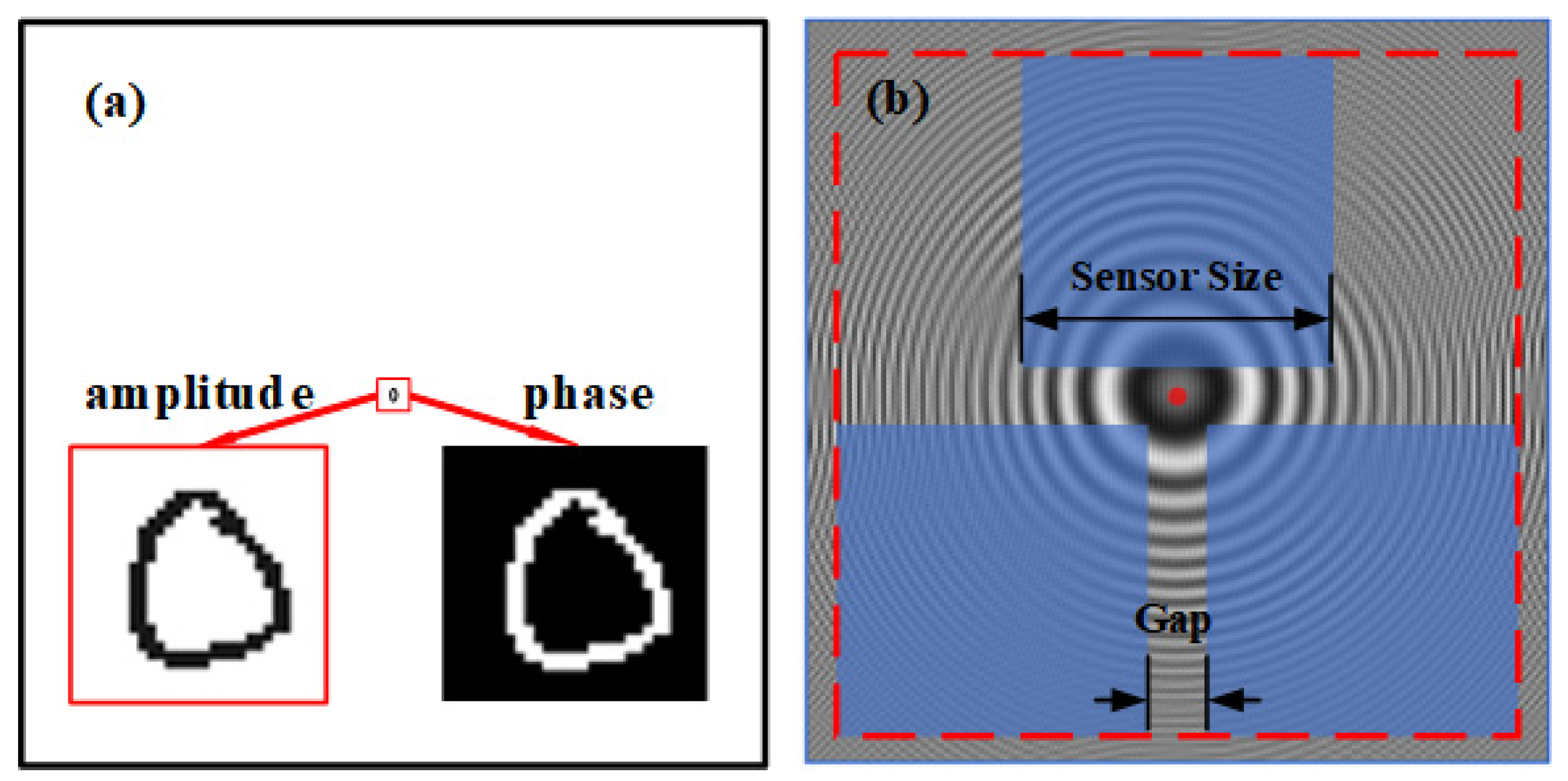
In the realm of DH, considering the constraints of sensor pixel pitch, the diffracted beam originating from each point on the object can be seen as a cone-shaped diffraction cone. The maximum spatial frequency that a sensor can capture is limited. As illustrated in Figure 2a, the target with the amplitude and the phase acquires the holographic field through digital holographic imaging. The blue section in Figure 2b is derived from sparse sampling by the sensor. Due to the inability of a full-field sensor to capture the entire image map effectively, a sparse sensor array is employed for collection. During the reconstruction of the image with the sparse sensor array, the loss of information from sensor gaps results in the loss of the frequency component corresponding to the entire scene. Hence, these sampling gaps exert an influence on the reconstructed amplitude and phase distributions of the object.

The digital holographic challenge posed by sparse aperture arrays can be transformed into hologram recovery problems involving sparse sampling, as depicted in the following equation:

$$M=W\odot I$$

(11)

where $W$ represents the sparse sampling matrix related to sensor sequence arrangement, $\odot$ denotes the Hadamard product, which is the element-wise multiplication of corresponding entries of two matrices. $I$ is the holographic field on the sensor and $M$ is the sparse sampled hologram.

Inspired by the transformation of the above problem, the HoloDiffusion method is proposed to improve the quality of reconstructed images. A detailed flowchart of the HoloDiffusion is illustrated in Figure 3.

During the prior learning stage, the gradient distribution of amplitude and phase is learned by denoising score-matching. Notably, the amplitude and phase of the object $O$ specifically are represented as the matrix $O=[O_{amp},O_{pha}]$ of the dual-channel. The HoloDiffusion is trained with $O$ in high-dimensional space as a network input, resulting in the acquisition of the parameterized $S_{\theta }(O,t)$.

In the iterative reconstruction stage, start with a hologram ${\widehat{I}}^{i+1}$ and turn to phase and amplitude through BP. A conversion of the hologram into amplitude and phase is necessary:

$$O^i=F^{-1}({\widehat{I}}^i)$$

(12)

where $F$ symbolizes the forward propagated (FP) process, and $F^{-1}$ corresponds to the backward propagation (BP) process. The estimated value of the hologram is denoted by ${\widehat{I}}^i$, and $O^i$ represents the estimated value of the amplitude and phase. Here, the superscript $i$ serves as an iteration marker during the reconstruction process. At the commencement of the reverse SDE stage, ${\widehat{I}}^{n-1}=M$.

For amplitude, the absorption constraint is implemented, and the amplitude is first inverted. This is because an object that absorbs light cannot have a negative value. In instances where the amplitude signifies light absorption, it is set to zero, necessitating the concurrent adjustment of the phase to zero at the corresponding location. Upon imposition of the constraint, the magnitude of negative values is multiplied by a matrix such that the pixel value of the hologram is 0, except for the support area. By using the prior information, the area with pixels set to 0 is negated, and the amplitude with a background of 1 is obtained. Therefore, the absorption constraint for amplitude $O_{amp}$ and the support constraint [26] for phase $O_{pha}$ are utilized to eliminate the twin image:

$$O_{amp}(x,y)=\left\{\begin{array}{ll}0,& (x,y)\in P\\ O_{amp}(x,y),& (x,y)\notin P\end{array}\right.$$

(13)

$$O_{pha}(x,y)=\left\{\begin{array}{ll}{O}_{pha}(x,y)/\left|O_{pha}(x,y)\right|,& \left|O_{pha}(x,y)\right|>1\\ O_{pha}(x,y),& \left|O_{pha}(x,y)\right|\le 1\end{array}\right.$$

(14)

where superscript $i$ is omitted for brevity, and $P$ represents pixels outside the support area.

Specifically, the continuous distribution over time is considered with diffusion processes. By inverting the SDE, random noise can be converted into data for sampling. The numerical solver employed for the inverse SDE functions as the predictor. In particular, the sample from the prior distribution can be obtained through the inverse SDE presented in Equation (8) and subsequently discretized in the following manner:

$$O^i=O^{i+1}+({\sigma }_{i+1}^2-{\sigma }_i^2)S_{\theta }(O^{i+1},{\sigma }_{i+1})+\sqrt{{\sigma }_{i+1}^2-{\sigma }_i^2}{z}_{i+1}$$

(15)

where $i=\mathrm{n}-1, \cdots , 1, 0$ is the number of discretization steps for the reverse-time SDE, ${\sigma }_i$ is the noise schedule at the $i\text{-}\mathrm{th}$ iteration, $z_{i+1}~N(0,1)$ denotes standard normalization, and $S_{\theta }(O^{i+1},{\sigma }_{i+1})$ is a score function with a time-conditional neural network.

After each iteration of the forward SDE, a fidelity operation is performed to ensure data consistency (DC):

$${\widehat{I}}^i=M\odot W+\mathrm{F}(O^i)\odot (1-W)$$

(16)

The hologram produced by the fidelity operation advances to the next iteration. The reconstructed amplitude and phase are derived via BP from the hologram in the final iteration. Additionally, the pseudo-code of the HoloDiffusion algorithm is depicted in Algorithm 1.

Algorithm 1 HoloDiffusion

Training stage 1: Dataset: $O=[O_{pha},O_{amp}]$ 2: Training $S_{\theta }(O,t)\simeq {\nabla }_O\log p_t(O)$ 3: Output: Trained HoloDiffusion $S_{\theta }(O,t)$

Reconstruction stage

Setting: $S_{\theta },N,\sigma ,\epsilon$

1: $O^N~N(0,{\sigma }_{\max }^2)$

2: For $i=n-1$ to 0 do

3:      Update $O^{i+1}$ by Equations (13) and (14)        (Constraints) 4:      $O^i\leftarrow \mathrm{Predictor} (O^i,{\sigma }_i,{\sigma }_{i+1})$ 5:      ${\widehat{I}}^i\leftarrow \mathrm{F}(O^i)$ 6:      Update $I^i$ by Equation (16)          (Data consistency) 7:      $O^i\leftarrow \mathrm{F}({\widehat{I}}^i)$

8: End for 9: Return $O^0$

After learning the distribution of the image set, the amplitude and the phase requiring reconstruction are input into the predictor, resulting in the generation of a reconstructed image, which is logged as an iteration. The phase and amplitude are converted into holograms through BP. Subsequently, the four blocks of the hologram are covered back for fidelity. Following numerous iterations, the ultimate reconstruction amplitude and phase are acquired.

3. Results

3.1. Data Specification

The dataset comprises 60,000 images, each featuring a resolution of 1200 × 1200 pixels and each pixel pitch is 3.8 μm. The central 28 × 28 pixel region of the image is generated using the MNIST dataset. For the amplitude, the digit portion is assigned a pixel value of 0.1 and the background portion is designated with a pixel value of 1. In the phase, the pixel values of the digit and the background are 1 and 0.

3.2. Model Training and Parameter Selection

The parameter selections are as follows: The wavelength is 500 nm, the side length of the object area is 0.001, the propagation distance is 0.0024, and the hologram side length is 0.001. During prior learning, the noise is added to the model is 2000 with a mean of 0 and a standard deviation that is a random number between 0.01 and 10. The random number seed used is set to 42. The model is trained by the Adam algorithm with a learning rate 0.0002. The method is implemented using a computer equipped with a NVIDIA TITAN GPU. To balance the quality of the reconstruction with the speed of the process, the iteration number is set to $n=500$ in the reconstruction stage.

3.3. Quantitative Indices

To quantitatively assess the quality of the reconstructed data, mean squared error (MSE), peak signal-to-noise ratio (PSNR), and structural similarity index (SSIM) are employed.

The MSE quantifies the error between paired observations that represent the same phenomenon. It is defined as follows:

$$\mathrm{MSE}(\widehat{O},\tilde{O})={\displaystyle \sum _{i=1}^{N_P}{‖{\widehat{O}}_i-{\tilde{O}}_i‖}_2}/N_P$$

(17)

where $N_P$ is the number of pixels within the reconstruction result, $\widehat{O}$ is the estimated value of the reconstructed phase or amplitude, and $\tilde{O}$ is the ground truth for comparison. As MSE approaches zero, it indicates that the reconstructed image is increasingly closer to the reference image.

PSNR describes the relationship between the maximum possible power of a signal and the power of noise corruption. A higher PSNR means better reconstruction quality. PSNR is expressed as follows:

$$\mathrm{PSNR}(\widehat{O},\tilde{O})=20\lg \left[\frac{\max (\tilde{O})}{\sqrt{\mathrm{MSE}(\widehat{O},\tilde{O})}}\right]$$

(18)

SSIM is utilized to measure the similarity between the ground-truth and reconstruction. It is represented as follows:

$$\mathrm{SSIM}(\widehat{O},\tilde{O})=\frac{(2{\mu }_{\widehat{O}}{\mu }_{\tilde{O}}+c_1)(2{\sigma }_{\widehat{O}\tilde{O}}+c_2)}{({\mu }_{\widehat{O}}^2+{\mu }_{\tilde{O}}^2+c_1)({\sigma }_{\widehat{O}}^2+{\sigma }_{\tilde{O}}^2+c_2)}$$

(19)

where ${\mu }_{\widehat{O}}$ and ${\sigma }_{\widehat{O}}^2$ are the average and variances of $\widehat{O}$. ${\sigma }_{\widehat{O}\tilde{O}}$ is the covariance of $\widehat{O}$ and $\tilde{O}$. $c_1$ and $c_2$ are used to maintain a stable constant.

3.4. Reconstruction at Gaps of Different Sizes

To evaluate the effectiveness of HoloDiffusion in reconstruction under various sensor gaps, experimental verification is carried out. Additionally, the reconstruction results are qualitatively and quantitatively compared with the SRSAA.

In the experiments, four sensors were used to detect the area corresponding to the blue sections, as shown in Figure 4. The four sensors were symmetrically distributed at the four corners of the holographic field, with gaps for every two sensors. The sensor size was specified as 450 × 450, and the size of the entire hologram was 1200 × 1200. In the iteration using the diffusion model, the reconstruction targets were cropped to amplitude and phase images with a resolution of 512 × 512 pixels due to the memory size limitations of the graphics card. Under the aforementioned fixed conditions, the effects of images reconstructed using the HoloDiffusion and SRSAA methods under various gap conditions were confirmed.

As depicted in Figure 5, the quality of the phase and amplitude reconstructed by both methods gradually deteriorates as the gap increases. However, HoloDiffusion demonstrates clearer results compared to SRSAA as the gap size increases, indicating improved performance when dealing with sparser sensor configurations. SRSAAs can achieve satisfactory reconstruction with a small gap size; as the gap size widens, more artifacts become apparent in SRSAAs. Compared to SRSAAs, the reconstructed amplitude and phase produced using HoloDiffusion exhibit superior image quality. For instance, when the gap size is 90, the reconstructed image using HoloDiffusion appears clearer and exhibits significantly reduced artifacts. The image reconstructed using the SRSAA method exhibits a loss of most target pixel details, and the linked regions are disjointed. Conversely, the images reconstructed using the HoloDiffusion method closely resemble the real situation while maintaining the details and leaving the structures unchanged.

As shown in

Table 1. The table shows the quantitative reconstruction results at different sensor gaps.

Gap	Type	SRSAA [dB/NA/NA]	HoloDiffusion [dB/NA/NA]
60	Phase	28.44/0.7997/0.0022	35.90/0.9149/0.0003
	Amplitude	37.03/0.9933/0.0002	41.89/0.9968/0.0001
90	Phase	29.28/0.7893/0.0014	35.51/0.9049/0.0009
	Amplitude	35.09/0.9833/0.0004	41.62/0.9955/0.0002
120	Phase	21.95/0.7327/0.0108	33.14/0.8462/0.0072
	Amplitude	29.24/0.9519/0.0018	38.93/0.9684/0.0035
150	Phase	16.58/0.6153/0.0315	29.53/0.7702/0.0145
	Amplitude	23.03/0.8521/0.0087	34.64/0.9299/0.0094
180	Phase	14.67/0.5204/0.0424	26.39/0.7012/0.0236
	Amplitude	20.50/0.7861/0.0157	30.97/0.8996/0.0153

, the average PSNR, SSIM, and MSE values of 100 images reconstructed from the MNIST dataset are recorded. HoloDiffusion can achieve notable average PSNR gains of 6.16 dB, 6.38 dB, 10.44 dB, 12.28 dB, and 11.10 dB at various gaps. What is exciting is that when the size of the gap is 90, the phase and amplitude reconstructed by the PSNR can attain 35.51 dB and 41.62 dB, respectively. Simultaneously, in comparison with the SRSAA method, the reconstruction results of HoloDiffusion display higher SSIM values and smaller MSE values. Hence, under the condition of larger gap size, HoloDiffusion demonstrates significant advancements in suppressing noise and artifacts.

3.5. Reconstruction under Different Numbers of Sensors

To confirm the effectiveness and robustness of the HoloDiffusion method in reconstructing images with varying numbers of sensors (SN), a comparison is made between the HoloDiffusion method and the SRSAA method.

In the experiments in this section, the gap was 120, and the sensor size was 500. A different number of sensors is used for various distributions, as depicted in Figure 6. Under the above fixed conditions, the effects of the images reconstructed by the HoloDiffusion and SRSAA methods are verified under the condition of different numbers of sensors.

As illustrated in Figure 7, a sharp decline in the quality of the reconstructed amplitude and phase is observed for both methods as the number of sensors decreases. While SRSAA is capable of reconstructing a clear image with a high number of sensors, its performance significantly deteriorates as the sensor count decreases, deviating from the ground truth in terms of basic outlines and details. As the number of sensors decreases, the image reconstructed by HoloDiffusion is clearer than that of the SRSAA. Furthermore, when the basic structure and outline of the image remain unchanged, the reconstructed image can more closely approach the ground truth. Experiments with varying sensor numbers demonstrate that HoloDiffusion not only reconstructs image details more effectively but also suppresses the generation of artifacts and twin images.

The average PSNR, SSIM, and MSE values of 100 images reconstructed from the MNIST dataset with different numbers of sensor arrays are documented in

Table 2. The table shows the quantitative reconstruction results with different numbers of sensors.

SN	Type	SRSAA [dB/NA/NA]	HoloDiffusion [dB/NA/NA]
2	Phase	11.55/0.2305/0.0742	11.61/0.2430/0.0735
	Amplitude	12.36/0.4862/0.0643	12.99/0.5571/0.0568
3	Phase	8.61/0.1239/0.1426	16.72/0.4327/0.0591
	Amplitude	18.06/0.7777/0.0204	24.85/0.9260/0.0085
4	Phase	15.58/0.5822/0.0300	34.16/0.8721/0.0021
	Amplitude	26.89/0.8879/0.0022	40.43/0.9934/0.0005

. In general, HoloDiffusion consistently outperforms across various sensor counts. Among them, when the number of sensors is three, the PSNR values of the phase and amplitude reconstructed by HoloDiffusion are improved by 8.11 dB and 6.79 dB. Furthermore, the reconstruction results obtained using the HoloDiffusion method demonstrate higher SSIM values and smaller MSE values. Even with fewer sensors, HoloDiffusion effectively suppresses noise and twin images to a significant extent.

3.6. Generalizability Verification on Cross-Dataset

A pre-trained diffusion model is employed to evaluate the generalization capabilities of the model across various datasets. The effectiveness and robustness of both methods are gauged.

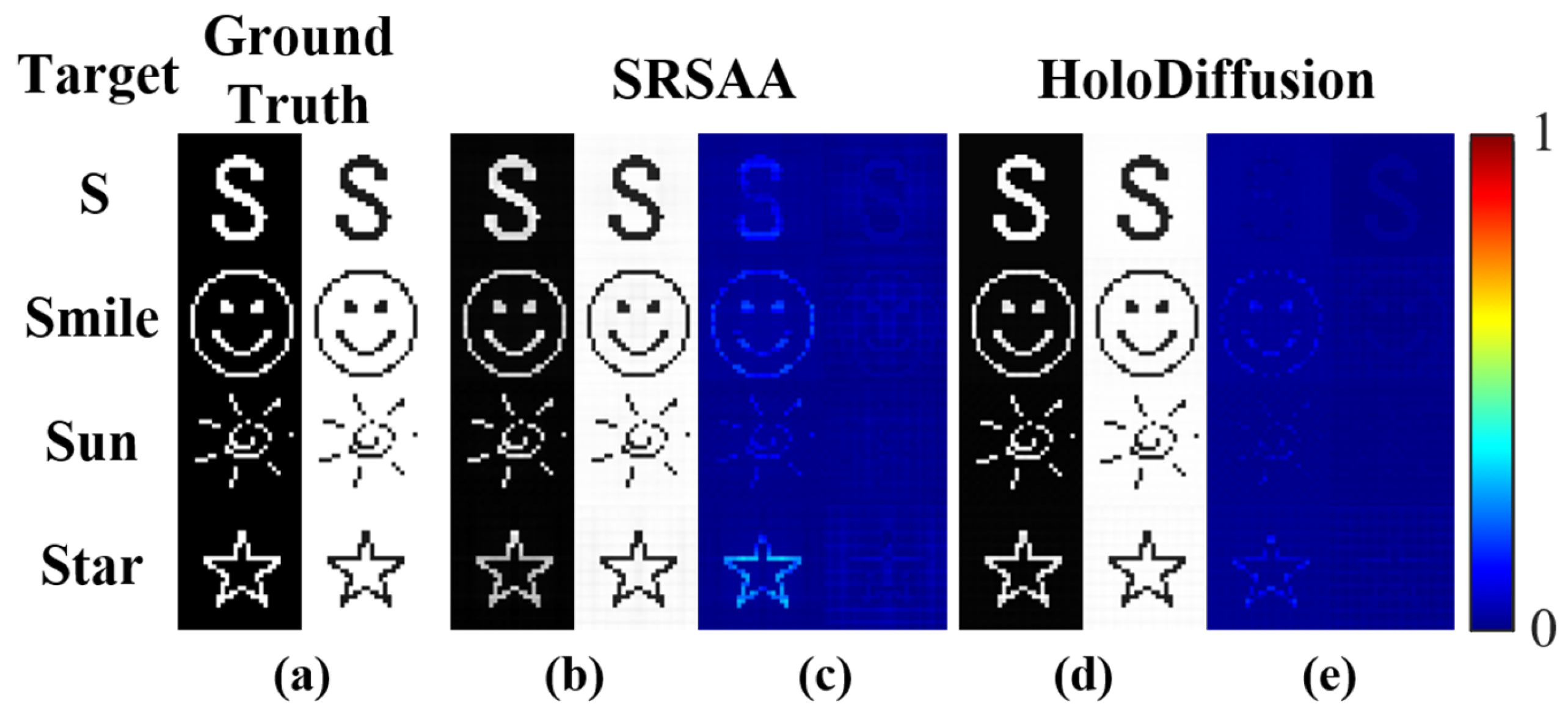
For visual comparison, the reconstructed images are presented in Figure 8. The HoloDiffusion method demonstrates fewer artifacts and maintains better continuity of image features compared to the SRSAA on cross-dataset. Regardless of whether it is analyzing phase or amplitude information, the HoloDiffusion method showcases improved reconstruction that more accurately mirrors the ground truth.

As listed in

Table 3. The table shows the quantitative reconstruction results on a cross-dataset.

Target	Type	SRSAA [dB/NA/NA]	HoloDiffusion [dB/NA/NA]
S	Phase	27.92/0.8939/0.0016	41.46/0.9611/0.0001
	Amplitude	33.62/0.9885/0.0004	45.05/0.9992/0.0000
Smile	Phase	25.10/0.9793/0.0031	30.68/0.9933/0.0009
	Amplitude	31.96/0.9966/0.0006	37.68/0.9996/0.0002
Sun	Phase	31.32/0.9467/0.0007	36.01/0.9419/0.0003
	Amplitude	36.47/0.9969/0.0002	42.11/0.9992/0.0001
Star	Phase	22.37/0.8049/0.0058	30.87/0.9076/0.0008
	Amplitude	30.95/0.9722/0.0008	36.80/0.9868/0.0002

, the HoloDiffusion method consistently outperforms the SRSAA in terms of performance, spanning almost all assessed datasets and metrics. Remarkably, the HoloDiffusion method achieves substantially elevated PSNR values, exhibiting an improvement margin of nearly 14 dB in certain cases. This suggests a significantly enhanced image reconstruction quality when employing the HoloDiffusion method. The SSIM outcomes indicate that HoloDiffusion excels in preserving structural integrity compared to the SRSAA. Furthermore, the lower MSE values imply a more accurate approximation to the original image in HoloDiffusion, indicating fewer errors during the reconstruction process.

Collectively, these results emphasize the exceptional performance of the HoloDiffusion method in image reconstruction, highlighting its potential for robust application across diverse imaging scenarios.

4. Discussion

4.1. Reconstruction at Different Sensor Sizes

In order to verify the effectiveness and robustness of the HoloDiffusion method in image reconstruction, sensor arrays with different sizes are used while maintaining a fixed gap.

As detailed in Figure 9, in the image reconstructed using the SRSAA method, a significant loss of detail is observed, and the connected areas appear fragmented or broken. The images reconstructed using the HoloDiffusion method are very close to the real situation while keeping the details and structures unchanged. As the sensor array size increases, the reconstructed images exhibit fewer artifacts and greater detail. It is obvious that the HoloDiffusion method achieves better results.

Table 4. The table shows the quantitative reconstruction results with different sensor array sizes.

Size	Type	SRSAA [dB/NA/NA]	HoloDiffusion [dB/NA/NA]
350	Phase	11.46/0.2372/0.0752	11.83/0.2782/0.0702
	Amplitude	13.36/0.5131/0.0550	13.44/0.5833/0.0510
400	Phase	11.95/0.2917/0.0677	13.71/0.4010/0.0559
	Amplitude	15.31/0.5984/0.0382	15.97/0.7153/0.0353
450	Phase	13.38/0.4181/0.0514	22.27/0.6083/0.0332
	Amplitude	18.52/0.7179/0.0209	26.35/0.8425/0.0212
500	Phase	14.67/0.5204/0.0424	26.39/0.7012/0.0236
	Amplitude	20.50/0.7861/0.0157	30.97/0.8996/0.0153

presents the average PSNR, SSIM, and MSE values for 100 images reconstructed from the MNIST dataset using a sensor count of four and a gap size of 180. The best PSNR, SSIM and MSE values achieved using different methods are highlighted in bold. With sensor sizes of 350, 400, 450, and 500, HoloDiffusion demonstrates an impressive average PSNR gain of 5.22 dB. Remarkably, when the sensor array size is 500, 11.10 dB can be achieved by the HoloDiffusion method. At the same time, compared with the SRSAA method, the reconstruction results of the HoloDiffusion method have higher SSIM values and smaller MSE values. Consequently, HoloDiffusion provides considerable improvements in noise and artifact suppression.

4.2. Reconstruction under Large Pixel Sizes

To evaluate the effectiveness of the HoloDiffusion method in reconstructing images with limited information, this section examines its performance using larger pixel sizes. Specifically, while maintaining the size of the single sensor, each pixel size is doubled from the original, which is equivalent to under-sampling.

For visual comparison, Figure 10 shows that the structure and contour of the amplitude and phase reconstructed by the HoloDiffusion method are closer to the real situation when the sampling rate is increased. The problem of part resolution reduction of the image can be further solved by using the HoloDiffusion method. In addition, at low sampling rates (SRs), the reconstructed HoloDiffusion amplitude outperforms the phase. It is hypothesized that this phenomenon can be attributed to the phase being more influenced by the amount of information than the amplitude.

Table 5. The table shows the quantitative reconstruction results at different sampling rates.

SR	Type	SRSAA [dB/NA/NA]	HoloDiffusion [dB/NA/NA]
1	Phase	21.95/0.7327/0.0108	33.14/0.8462/0.0072
	Amplitude	29.24/0.9519/0.0018	38.93/0.9684/0.0035
5/6	Phase	19.85/0.6760/0.0171	28.71/0.7581/0.0158
	Amplitude	27.16/0.9294/0.0027	33.93/0.9275/0.0089
4/5	Phase	19.61/0.6687/0.0177	28.41/0.7553/0.0166
	Amplitude	26.99/0.9257/0.0029	33.64/0.9271/0.0090

tabulates the average PSNR, SSIM, and MSE values of 100 images reconstructed from the MNIST dataset. Compared to the SRSAA method, the HoloDiffusion method produces reconstruction results with superior SSIM and PSNR values. It can be seen that at a sampling rate of 4/5, images reconstructed via the HoloDiffusion method begin to demonstrate better results.

5. Conclusions

In the context of digital hologram reconstruction, an algorithm is proposed founded on a diffusion model characterized by robust generative abilities. The diffusion model is incorporated into the physics-based iterative reconstruction process, specifically for image rotation in the SRSAA method. This integration enables the execution of image generation on the amplitude image within the holographic domain. Specifically, amplitude and phase information for both channels of the holographic domain image is obtained using diffusion modeling. After under-sampling the image, the SRSAA is utilized to ensure the fidelity of the phase and amplitude. The phase and amplitude are put into the network based on the prior information for prediction. The numerical SDE solution is executed alternately during the iteration stage, allowing for the acquisition of generated sample data and facilitating efficient reconstruction. The image reconstruction and model generation capabilities were validated, and this method demonstrated superior reconstruction effects under four new image sampling methods. The results indicate that the model exhibits greater flexibility in handling complex holographic image reconstruction and has broader applicability in diverse digital images.

References

- Schnars, U.; Jüptner, W. Direct recording of holograms by a CCD target and numerical reconstruction. Appl. Opt. 1994, 33, 179–181. [Google Scholar] [CrossRef] [PubMed]
- Schnars, U.; Jüptner, W. Digital recording and numerical reconstruction of holograms. Meas. Sci. Technol. 2002, 13, R85. [Google Scholar] [CrossRef]
- De Nicola, S.; Finizio, A.; Pierattini, G.; Ferraro, P.; Alfieri, D. Angular spectrum method with correction of anamorphism for numerical reconstruction of digital holograms on tilted planes. Opt. Express 2005, 13, 9935–9940. [Google Scholar] [CrossRef] [PubMed]
- Javidi, B.; Tajahuerce, E. Three-dimensional object recognition by use of digital holography. Opt. Lett. 2000, 25, 610–612. [Google Scholar] [CrossRef] [PubMed]
- Javidi, B.; Tajahuerce, E. Tracking biological microorganisms in sequence of 3D holographic microscopy images. Opt. Express 2007, 15, 10761–10766. [Google Scholar]
- Kemper, B.; Bally, G. Digital holographic microscopy for live cell applications and technical inspection. Appl. Opt. 2008, 47, A52–A61. [Google Scholar] [CrossRef]
- Di, J.; Li, Y.; Xie, M.; Zhang, J.; Ma, C.; Xi, T.; Li, E.; Zhao, J. Dual-wavelength common-path digital holographic microscopy for quantitative phase imaging based on lateral shearing interferometry. Appl. Opt. 2016, 55, 7287–7293. [Google Scholar] [CrossRef] [PubMed]
- Cuche, E.; Marquet, P.; Depeursinge, C. Simultaneous amplitude-contrast and quantitative phase-contrast microscopy by numerical reconstruction of Fresnel off-axis holograms. Appl. Opt. 1999, 38, 6994–7001. [Google Scholar] [CrossRef]
- Pourvais, Y.; Asgari, P.; Abdollahi, P.; Khamedi, R.; Moradi, A. Microstructural surface characterization of stainless and plain carbon steel using digital holographic microscopy. J. Opt. Soc. Am. B 2017, 34, B36–B41. [Google Scholar] [CrossRef]
- Thurman, S.T.; Bratcher, A. Multiplexed synthetic-aperture digital holography. Appl. Opt. 2015, 54, 559–568. [Google Scholar] [CrossRef]
- Luo, W.; Greenbaum, A.; Zhang, Y.B.; Ozcan, A. Synthetic aperture-based on-chip microscopy. Light Sci. Appl. 2015, 4, e261. [Google Scholar] [CrossRef]
- Latychevskaia, T.; Fink, H.W. Resolution enhancement in digital holography by self-extrapolation of holograms. Opt. Express 2013, 21, 7726–7733. [Google Scholar] [CrossRef] [PubMed]
- Latychevskaia, T.; Fink, H.W. Coherent microscopy at resolution beyond diffraction limit using post-experimental data extrapolation. Appl. Phys. Lett. 2013, 103, 204105. [Google Scholar] [CrossRef]
- Huang, Z.; Cao, L. Bicubic interpolation and extrapolation iteration method for high resolution digital holographic reconstruction. Opt. Lasers Eng. 2020, 130, 106090. [Google Scholar] [CrossRef]
- Huang, H.; Rong, L.; Wang, D.; Li, W.; Deng, Q.; Li, B.; Wang, Y.; Zhan, Z.; Wang, X.; Wu, W. Synthetic aperture in terahertz in-line digital holography for resolution enhancement. Appl. Opt. 2016, 55, A43–A48. [Google Scholar] [CrossRef]
- Li, Z.; Zou, R.; Kong, W.; Wang, X.; Deng, Q.; Yan, Q.; Qin, Y.; Wu, W.; Zhou, X. Terahertz synthetic aperture in-line holography with intensity correction and sparsity autofocusing reconstruction. Photonics Res. 2019, 7, 1391–1399. [Google Scholar] [CrossRef]
- Gerchberg, R.W.; Saxton, W.O. A practical algorithm for the determination of phase from image and diffraction plane pictures. Optik 1972, 35, 237–246. [Google Scholar]
- Fienup, J.R. Phase retrieval algorithms: A comparison. Appl. Opt. 1982, 21, 2758–2769. [Google Scholar] [CrossRef]
- Huang, Z.; Cao, L. Faithful digital holographic reconstruction using a sparse sensor array. Appl. Phys. Lett. 2020, 117, 031105. [Google Scholar] [CrossRef]
- Song, Y.; Ermon, S. Generative modeling by estimating gradients of the data distribution. Adv. Neural Inf. Process. Syst. 2019, 32. [Google Scholar] [CrossRef]
- Wang, S.; Lv, J.; He, Z.; Liang, D.; Chen, Y.; Zhang, M.; Liu, Q. Denoising auto-encoding priors in undecimated wavelet domain for MR image reconstruction. Neurocomputing 2021, 37, 325–338. [Google Scholar] [CrossRef]
- Liu, X.; Zhang, M.; Liu, Q.; Xiao, T.; Zheng, H.; Ying, L.; Wang, S. Multi-contrast MR reconstruction with enhanced denoising autoencoder prior learning. In Proceedings of the 2020 IEEE 17th International Symposium on Biomedical Imaging (ISBI), Iowa City, IA, USA, 3–7 April 2020; IEEE: Piscataway, NJ, USA, 2020; pp. 1–5. [Google Scholar]
- Avrahami, O.; Lischinski, D.; Fried, O. Blended diffusion for text-driven editing of natural images. In Proceedings of the IEEE/CVF Conference on Computer Vision and Pattern Recognition, New Orleans, LA, USA, 18–24 June 2022; pp. 18208–18218. [Google Scholar]
- Daniels, M.; Maunu, T.; Hand, P. Score-based generative neural networks for large-scale optimal transport. Adv. Neural Inf. Process. Syst. 2021, 34, 12955–12965. [Google Scholar]
- Anderson, B.D.O. Reverse-time diffusion equation models. Stoch. Process. Their Appl. 1982, 12, 313–326. [Google Scholar] [CrossRef]
- Gao, Y.; Cao, L. Iterative projection meets sparsity regularization: Towards practical single-shot quantitative phase imaging with in-line holography. Light Adv. Manuf. 2023, 4, 37–53. [Google Scholar] [CrossRef]
Figure 1.
The figure shows that the data perturbed by noise is smoothed along the trajectory of a SDE. By estimating the score function using a SDE, it is possible to approximate the reverse SDE and subsequently solve it, enabling the generation of image samples from noise.
Figure 2.
The figure shows a sparse aperture digital holography. (a) The insertion plot depicts the amplitude and phase of the target. (b) Holographic field and sparse sensor distribution; the blue part represents the position of the sensor.
Figure 3.
The figure shows the proposed method for digital holographic reconstruction. (Top): Prior learning stage to learn the gradient distribution via denoising score matching. (Bottom): Iterate between numerical SDE solver and data-consistency step to achieve reconstruction.
Figure 4.
The figure shows the sensor distribution at different distances. The blue squares represent sensor arrays.
Figure 5.
The figure shows the reconstruction results using different methods at sensor array sizes equal to 450 and different gaps. (a) Ground truth, (b) SRSAA, (c) residual image between (a) and (b), (d) HoloDiffusion, (e) residual image between (a) and (d).
Figure 6.
The figure shows the distribution of different numbers of sensors. The blue squares represent sensor arrays. (a–c) represent the sampling conditions when the number of sensors is 2, 3, and 4, respectively.
Figure 7.
The figure shows the reconstruction results using different methods with a sensor array size equal to 500, a gap equal to 120, and different numbers of sensors. (a) Ground truth, (b) SRSAA, (c) residual image between (a) and (b), (d) HoloDiffusion, (e) residual image between (a) and (d).
Figure 8.
The figure shows the reconstruction results using different methods with a sensor array size equal to 500 and gap equal to 120 on cross-dataset. (a) Ground truth, (b) SRSAA, (c) residual image between (a) and (b), (d) HoloDiffusion, (e) residual image between (a) and (d).
Figure 9.
The figure shows the reconstruction results using different methods at different sensor array sizes and gap equal to 180. (a) Ground truth, (b) SRSAA, (c) residual image between (a) and (b), (d) HoloDiffusion, (e) residual image between (a) and (d).
Figure 10.
The figure shows the reconstruction results using different methods at different sampling rates with a sensor size equal to 500 and gap equal to 120. (a) Ground truth, (b) SRSAA, (c) residual image between (a) and (b), (d) HoloDiffusion, (e) residual image between (a) and (d).