Performance Analysis of Optical Spatial Modulation in Atmospheric Turbulence Channel ^†

Abstract

In this paper, spatial pulse position modulation (SPPM) is used as a case study to investigate the performance of the optical spatial modulation (SM) technique in outdoor atmospheric turbulence (AT). A closed-form expression for the upper bound on the asymptotic symbol error rate (SER) of SPPM in AT is derived and validated by closely-matching simulation results. The error performance is evaluated in weak to strong AT conditions. As the AT strength increases from weak to strong, the channel fading coefficients become more dispersed and differentiable. Thus, a better error performance is observed under moderate-to-strong AT compared to weak AT. The performance in weak AT can be improved by applying unequal power allocation to make free-space optical communication (FSO) links more distinguishable at the receiver. Receive diversity is considered to mitigate irradiance fluctuation and improve the robustness of the system to turbulence-induced channel fading. The diversity order is computed as half of the number of detectors. Performance comparisons, in terms of energy and spectral efficiencies, are drawn between the SPPM scheme and conventional MIMO schemes such as repetition coding and spatial multiplexing.

1. Introduction

Free-space optical communication (FSO) technology is a promising complement to existing radio frequency communications. In addition to its huge bandwidth resource and its potential to support gigabit rate throughput, the FSO system can be deployed using low-power and low-cost components [1,2]. The major drawback of the FSO technology is its dependence on atmospheric conditions, which affects link availability. Variations in pressure and temperature create random changes in the refractive index of the atmosphere. This leads to atmospheric turbulence (AT)-induced fluctuation in the received irradiance [3,4,5]. In order to enhance capacity, reliability, and/or coverage, multiple-input multiple-output (MIMO) techniques are employed to exploit additional degrees of freedom, such as the space and emitted colour of the optical sources and the field of view of the detectors. FSO systems using MIMO diversity techniques are explored in [4,6,7] to mitigate the effect of turbulence-induced fading by providing redundancy. In this paper, we consider the use of a low-complexity MIMO technique, known as spatial modulation (SM) [8,9], to enhance the spectral efficiency of FSO systems. The SM technique achieves higher spectral efficiency by encoding additional information bits in the spatial domain of the multiple optical sources at the transmitter.

Multiple variants of SM have been explored in FSO systems, using different statistical distributions to model the channel fading [10,11,12,13,14,15]. A variant of optical SM (OSM) termed space shift keying (SSK) is studied in [10,11,12]. In the SSK scheme, no digital signal modulation is used, and the information bits are encoded solely on the spatial index of the optical sources. Our paper differs from these previous works in that we have considered a full-fledged OSM scheme, which entails using both the spatial index of the sources and the transmitted digital signal modulation to convey the information bits. The work in [13] is related to ours, as it considered an OSM scheme in which digital signal modulation is also employed. However, the analytical framework included kernel density estimation, which does not provide a closed-form solution. Using the homodyned-K (HK) distribution to model turbulence-induced fading, the performance of outdoor OSM (SSK) with coherent detection was reported in [14]. Furthermore, authors [16] considered power series-based analysis of the effect of misalignment and Gamma-Gamma turbulence fading on the SM technique with BPSK constellation

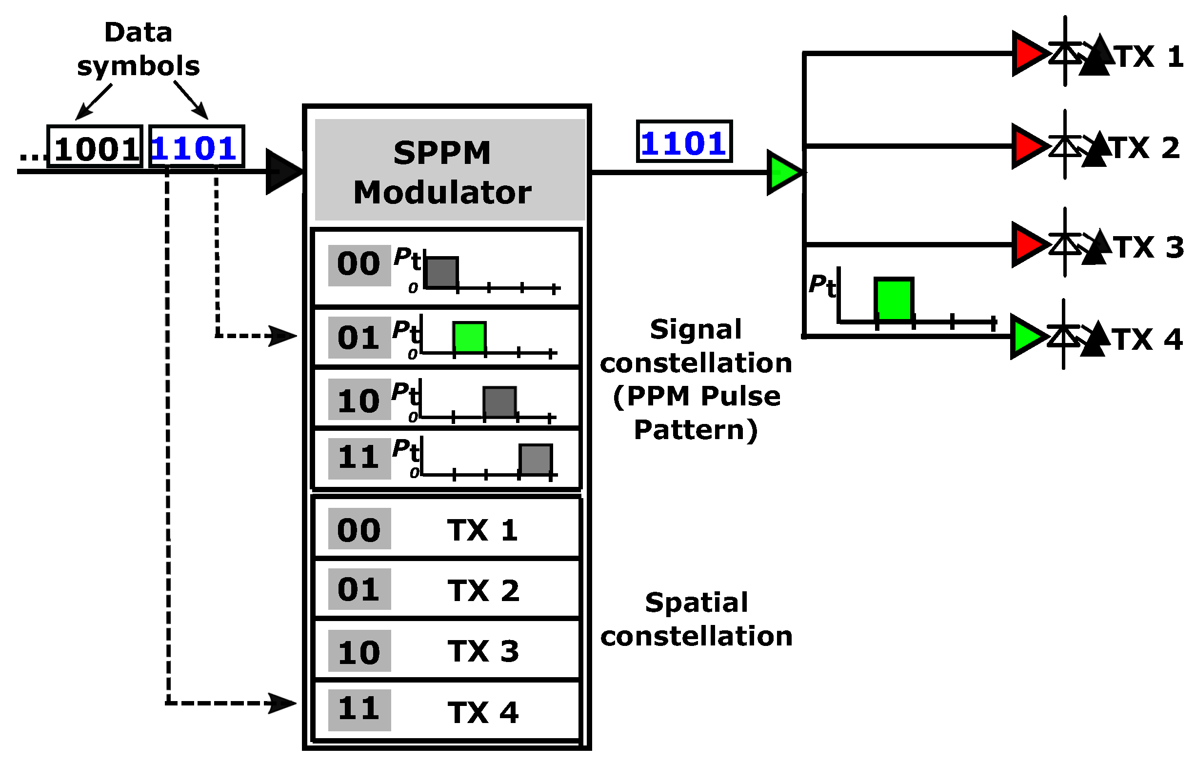
Given that AT primarily affects the emitted light intensity, pulse position modulation (PPM) is commonly used in an FSO system because, unlike on-off keying (OOK) and pulse-amplitude modulation (PAM), its detection process is not reliant on the channel states [3]. Nevertheless, PPM is limited by its poor spectral efficiency, which is due to its high bandwidth requirement. In order to enhance the spectral efficiency of PPM, a variant of the OSM technique termed spatial pulse position modulation (SPPM) [17] is explored in this paper. SPPM is a MIMO scheme in which out of $N_{\mathrm{t}}$ transmit units (TXs), i.e., optical sources, only one is activated to send the data signal during a symbol period. Then, in addition to the bits sent by the transmitted PPM signal, extra bits are encoded on and conveyed by the spatial index of the activated TX. Thus, SPPM transmits more bits/symbol and therefore has higher spectral efficiency than PPM. Moreover, SPPM benefits from the power efficiency of the transmitted PPM signal. Furthermore, compared to other classical MIMO techniques like spatial multiplexing (SMX), in SM schemes such SPPM, since only one TX is active in any symbol duration, the transceiver implementation is less complex and more flexible. For instance, SMX requires that the number of receiver detectors should be at least equal to the number of TX, a condition that is not mandatory for SPPM. Furthermore, inter-channel interference (ICI) due to multiple data streams in SMX is avoided in SPPM, and this reduces its detection complexity.

In this work, the performance of an SPPM-based FSO system is evaluated under weak to strong AT conditions. The intensity fluctuations caused by AT are modelled by the Gamma-Gamma (GG) distribution, which is widely adopted to study FSO links under weak to strong AT conditions, because it matches the experimental results [1,18]. The contributions of this paper include: (1) the theoretical expression for the upper bound on the asymptotic symbol error rate (SER) of SPPM in FSO channels is derived and validated by closely matching simulation results. (2) As the AT strength increases from weak to strong, the distribution of the fading coefficients spreads out more. Thus, the influence of the dispersion of the coefficients on the error performance of OSM schemes is explored under different AT conditions. (3) Furthermore, since SM provides increased throughput, but not transmit diversity gain, spatial diversity is considered at the receiver in order to improve the system performance, and the diversity gain of the multiple-detector system is obtained from the error plots. (4) The performance of the SPPM scheme is also compared to that of SSK and other conventional MIMO schemes such as repetition coding (RC) and SMX. The performance comparison is presented in terms of energy and spectral efficiencies.

The rest of the paper is organized as follows. The system and channel models are provided in Section 2. In Section 3, the theoretical derivation of the upper bound on asymptotic SER of SPPM in GG FSO channels is presented. The results of the performance evaluation are provided and discussed in Section 4, and our concluding remarks are given in Section 5.

2. System and Channel Model

2.1. The SPPM Scheme

Considering an $N_{\mathrm{t}}\times N_{\mathrm{r}}$ optical MIMO system with $N_{\mathrm{t}}$ TXs, i.e., light-emitting diodes (LEDs) or lasers, and $N_{\mathrm{r}}$ receive units (RXs), i.e., PINphotodetectors (PDs), by using the SPPM scheme [17], only one of the TXs is activated in a given symbol duration, while the rest of the TXs are idle. The activated source transmits an L-PPM signal pattern, where L denotes the number of time slots (chips) in a symbol duration. A total of $M={\log }_2\left(N_{\mathrm{t}}L\right)$ bits is transmitted per data symbol. The first ${\log }_2\left(N_{\mathrm{t}}\right)$ most significant bits are encoded in the index (position) of the activated TX, while the remaining ${\log }_2\left(L\right)$ bits are conveyed by the pulse position in the transmitted PPM signal. The SPPM encoding is further illustrated in Figure 1 for the case of $N_{\mathrm{t}}=4$ and $L=4$. For instance, to transmit the symbol ‘13’ with binary representation ‘1101’, the two most significant bits, ‘11’, are used to select ‘TX 4’, while the last two bits, ‘01’, indicate that the pulse will be transmitted in the second time slot of the four-PPM pulse pattern.

The signal emitted by the activated TX propagates through the FSO channel to the receiver. Due to the spatial separation of the TXs, each of them introduces a specific “channel signature”, which makes its emitted signal unique at the RX compared to the same signal emitted by any other TX. The detection unit at the receiver exploits the unique signatures of each TX to retrieve the sent information bits. Typical of communication systems, especially in MIMO systems where knowledge of the channel state is required, the channel coefficients are assumed to be known at the RX. Based on the channel coefficients, the demodulator performs a maximum likelihood detection and makes a decision in favour of the TX index and PPM pulse position combination with the lowest Euclidean distance from the received signal [17,19].

2.2. SPPM System Model

The following notations are used throughout the paper: bold lower-case fonts denote vectors, while the bold upper-case fonts represent matrices. Regular italicised fonts denote scalar parameters. Consider that a data symbol is transmitted by activating the jth LED, $1\le j\le N_{\mathrm{t}}$, to transmit a pulse in slot m, $0\le m\le (L-1)$, of the L-PPM signal; the $N_{\mathrm{r}}\times 1$ vector of received electrical signal over the symbol duration, T, is:

$$\mathbf{r}\left(t\right)={\omega }_{j}R\mathbf{H}{\mathbf{s}}_{j,m}\left(t\right)+\mathbf{n}\left(t\right),0\le t\le T,$$

(1)

where R is the responsivity of the PD. The parameter ${\omega }_j$ for $j=1,\dots ,N_{\mathrm{t}}$, are weights that can be applied to induce power imbalance between the TXs in order to improve their differentiability at the receiver. The $N_{\mathrm{r}}\times N_{\mathrm{t}}$ FSO channel matrix is represented by $\mathbf{H}$. The quantity $\mathbf{n}\left(t\right)$ is the sum of the ambient light shot noise and the thermal noise in the $N_{\mathrm{r}}$ PIN PDs, and it is modelled as independent and identically distributed (i.i.d) additive white Gaussian noise (AWGN) with variance ${\sigma }^2=N_0/2$; $N_0$ represents the noise power spectral density [1,20]. The $N_{\mathrm{t}}\times 1$ transmit signal vector, ${\mathbf{s}}_{j,m}\left(t\right)={[0,\dots ,s_{j,m}\left(t\right),\dots ,0]}^{\mathcal{T}}$, has a nonzero entry at the index of the activated jth TX, where $\mathcal{T}$ denotes the transpose operation, and $s_{j,m}\left(t\right)$ is the transmitted L-PPM waveform, with a pulse of amplitude $P_{\mathrm{t}}$ in slot m.

The matched filter (MF) receiver architecture employs a unit-energy receive filter, and the output of the MF in each time slot is obtained by sampling at the chip rate, $1/T_{\mathrm{c}}$, where the duration of each time slot $T_{\mathrm{c}}=T/L$. Based on the maximum likelihood (ML) detection criterion, the estimate of the transmitted SPPM symbol is obtained from the combination of the pulse position and the TX index, which gives the minimum Euclidean distance from the received signal [17]. That is,

$$\begin{array}{cc}\hfill [\widehat{m},\widehat{j}]& =arg\underset{m,j}{max}{f}_r\left(\mathbf{r}\left(t\right)|{\mathbf{s}}_{j,m}\left(t\right),{\omega }_j,\mathbf{H}\right)\hfill \\ & =arg\underset{m,j}{min}{∥\mathbf{r}\left(t\right)-{\omega }_{j}R\mathbf{H}{\mathbf{s}}_{j,m}\left(t\right)∥}^2\hfill \end{array}$$

(2)

where $f_r\left(\mathbf{r}|{\mathbf{s}}_{j,m},{\omega }_j,\mathbf{H}\right)$ is the probability density function (PDF) of $\mathbf{r}\left(t\right)$ conditioned on ${\mathbf{s}}_{j,m}$ being transmitted, weight ${\omega }_j$, and channel matrix $\mathbf{H}$.

2.3. FSO Channel Model

As the transmitted signal propagates through the FSO channel, it experiences turbulence-induced channel fading, which is characterised by the GGdistribution [1,21]. The PDF of the GG fading coefficients is given by [21]:

$$f_H\left(h\right)=\frac{2{\left(\alpha \beta \right)}^{\frac{\alpha +\beta }{2}}}{\Gamma \left(\alpha \right)\Gamma \left(\beta \right)}{h}^{\frac{\alpha +\beta }{2}-1}{\mathrm{K}}_{\alpha -\beta }\left(2\sqrt{\alpha \beta h}\right)$$

(3)

where h is the fading coefficient. The functions $\Gamma (·)$ and ${\mathrm{K}}_{\nu }(·)$ denote the Gamma function and the modified Bessel function of the second kind of order $\nu$, respectively. The scalars $\alpha$ and $\beta$ are the scintillation parameters that characterize the intensity fluctuations, and they are related to the atmospheric conditions through the log-intensity variance ${\sigma }_l^2$. The values of $\alpha$, $\beta$, and ${\sigma }_l^2$ specified for different regimes of atmospheric turbulence are given in

Table 1. Atmospheric turbulence parameters [1].

Turbulence Level	${\mathit{\sigma }}_{\mathit{l}}^2$	$\mathit{\alpha }$	$\mathit{\beta }$
Weak	0.2	11.7	10.1
Moderate	1.6	4.0	1.9
Strong	3.5	4.2	1.4

from [1].

In order to provide a closed-form solution, the modified Bessel function in (3) is expressed in terms of the Meijer-G function, $G_{c,d}^{a,b}(·)$ by applying ([22], Equation (8.4.23.1)):

$$K_{\alpha -\beta }\left(2\sqrt{\alpha \beta h}\right)=\frac{1}{2}{G}_{0,2}^{2,0}\left(\alpha \beta h\right|\begin{array}{c}-\\ \frac{\alpha -\beta }{2},\frac{\beta -\alpha }{2}\end{array}),$$

(4)

to obtain:

$$f_H\left(h\right)=\frac{{\left(\alpha \beta \right)}^{\frac{\alpha +\beta }{2}}}{\Gamma \left(\alpha \right)\Gamma \left(\beta \right)}{h}^{\frac{\alpha +\beta }{2}-1}{G}_{0,2}^{2,0}\left(\alpha \beta h\right|\begin{array}{c}-\\ \frac{\alpha -\beta }{2},\frac{\beta -\alpha }{2}\end{array}).$$

(5)

To further simplify (5), we utilize the transformation ([22], Equation (8.2.2.15)):

$${\chi }^{\kappa }{G}_{p,q}^{m,n}\left(\chi \right|\begin{array}{c}\left(a_p\right)\\ \left(bq\right)\end{array})=G_{p,q}^{m,n}\left(\chi \right|\begin{array}{c}\left(a_p\right)+\kappa \\ \left(bq\right)+\kappa \end{array}),$$

(6)

for a given set of arbitrary parameters $\{\chi ,\kappa ,m,n,p,q,a_p,b_q\}$, and the Expression (5) is reduced to:

$$f_H\left(h\right)=\frac{\left(\alpha \beta \right)}{\Gamma \left(\alpha \right)\Gamma \left(\beta \right)}{G}_{0,2}^{2,0}\left(\alpha \beta h\right|\begin{array}{c}-\\ \alpha -1,\beta -1\end{array}).$$

(7)

It is assumed that the individual units in the transmitter and receiver arrays are spatially separated by at least the correlation width, $w_{\mathrm{c}}=\sqrt{\lambda d}$, such that the elements of the FSO channel matrix, $\mathbf{H}$, are independent and uncorrelated. The transmission wavelength and the link distance are denoted by $\lambda$ and d, respectively. This assumption is realistic because the transverse correlation width of the laser radiation in AT is typically on the order of a few centimetres [5,23]. For instance, in a FSO system with $\lambda =1.55\mathsf{\mu }$m and a link distance of $d=2.5$ km, for the received signals to be uncorrelated, the required spatial spacing is about $w_{\mathrm{c}}=6.2$ cm. Thus, we can infer that the proposed system model can be implemented with practical spacings between each unit of the transmit and receive arrays.

3. Performance Analysis of SPPM in FSO

As stated in Section 2.2, a transmitted data symbol is correctly detected if both the pulse position and the TX index are correctly detected. Thus, the symbol error probability of SPPM is given by:

$$P_{\mathrm{e},\mathrm{sym}}=1-\left(P_{\mathrm{c},\mathrm{tx}}\times P_{\mathrm{c},\mathrm{ppm}}\right),$$

(8)

where $P_{\mathrm{c},\mathrm{ppm}}$ is the probability of correctly detecting the PPM pulse position and $P_{\mathrm{c},\mathrm{tx}}$ is the probability of correctly detecting the index of the activated TX given that pulse position has been correctly detected. The expressions for $P_{\mathrm{c},\mathrm{ppm}}$ and $P_{\mathrm{c},\mathrm{tx}}$ are derived as follows.

3.1. Probability of Correct TX Index Detection

Consider that the transmitted data symbol is sent by activating TX j. For a given channel realization, $\mathbf{H}$, assuming a correct pulse position detection, the instantaneous pairwise error probability (PEP) that the receiver decides in favour of TX i instead of j is obtained by generalising the single-detector expression given by [17] to a multiple-detector scenario, and we obtain:

$${\mathrm{PEP}}_m^{j\to i}=\frac{1}{2}\mathrm{erfc}\left(\frac{\sqrt{{\gamma }_{\mathrm{s}}}}{2}\sum _{k=1}^{N_{\mathrm{r}}}\left|{\omega }_i{h}_{ik}-{\omega }_j{h}_{jk}\right|\right),$$

(9)

where $\mathrm{erfc}(·)$ denotes the complementary error function. The scalars $h_{ik}$ and $h_{jk}$ for $1\le i,j\le N_{\mathrm{t}}$ are the channel fading coefficients of the link between the kth PD and the TXs i and j, respectively. That is, $h_{ik}$ and $h_{jk}$ denote the entries on the ith and jth rows of the kth column of $\mathbf{H}$. The signal-to-noise ratio (SNR) per symbol ${\gamma }_{\mathrm{s}}=E_{\mathrm{s}}/N_0$, and the average energy per symbol $E_{\mathrm{s}}={\left(R{P}_{\mathrm{t}}\right)}^2{T}_{\mathrm{c}}$.

To simplify the analyses that follow, we define the random variable (RV):

$$\begin{array}{c}\hfill \psi =\sum _{k=1}^{N_{\mathrm{r}}}\left|{\omega }_i{h}_{ik}-{\omega }_j{h}_{jk}\right|.\end{array}$$

(10)

By applying (10), we express (9) as:

$${\mathrm{PEP}}_m^{j\to i}=\frac{1}{2}\mathrm{erfc}\left(\frac{\sqrt{\psi }}{2}\right),$$

(11)

and by averaging over the PDF of $\psi$, the average PEP (APEP) of correct TX index detection is given by:

$${\mathrm{APEP}}_m^{j\to i}=\frac{1}{2}{\int }_0^{\infty }\mathrm{erfc}\left(\frac{\sqrt{\psi }}{2}\right)f_{\psi }\left(\psi \right)\mathrm{d}\psi .$$

(12)

After some RV transformations and using the PDF of the GG fading coefficients given by (7), the PDF of variable $\psi$ is obtained as (A11) in Appendix A. Hence, we substitute (A11) in (12), and the integral relation ([24], (Equation (4.1.18)):

$${\int }_0^{\infty }\mathrm{erfc}\left(a\varphi \right){\varphi }^p\mathrm{d}\varphi =\frac{1}{(p+1)a^{p+1}\sqrt{\pi }}\Gamma \left(\frac{p}{2}+1\right),$$

(13)

for arbitrary scalars a, $\varphi$, and p, $\left|\arg \left\{a\right\}\right|<\pi /4,p<-1$, is applied to derive the asymptotic APEP of detecting the index of the activated TX as:

$$\begin{array}{cc}\hfill {\mathrm{APEP}}_m^{j\to i}& =\frac{2^{N_{\mathrm{r}}}\Gamma \left(\frac{N_{\mathrm{r}}+1}{2}\right)}{N_{\mathrm{r}}\Gamma \left(\frac{N_{\mathrm{r}}}{2}\right)}{\left(\frac{\alpha \beta }{{\omega }_i{\left(\Gamma \left(\alpha \right)\Gamma \left(\beta \right)\right)}^2\sqrt{{\gamma }_{\mathrm{s}}}}{G}_{3,3}^{2,3}\left(\frac{{\omega }_j}{{\omega }_i}\right|\begin{array}{c}0,1-\alpha ,1-\beta \\ \alpha -1,\beta -1,0\end{array})\right)}^{N_{\mathrm{r}}}.\hfill \end{array}$$

(14)

For $N_{\mathrm{t}}$ equiprobable TXs, using the union bound technique [25], the probability of correctly detecting the TX index conditioned on a correctly-detected pulse position is:

$$\begin{array}{cc}\hfill P_{\mathrm{c},\mathrm{tx}}& \le 1-\frac{1}{N_{\mathrm{t}}}\sum _{j=1}^{N_{\mathrm{t}}}\sum _{\begin{array}{c}i=1\\ i\ne j\end{array}}^{N_{\mathrm{t}}}{\mathrm{APEP}}_m^{j\to i}\hfill \\ & =1-\frac{1}{N_{\mathrm{t}}}\sum _{j=1}^{N_{\mathrm{t}}}\sum _{\begin{array}{c}i=1\\ i\ne j\end{array}}^{N_{\mathrm{t}}}\frac{2^{N_{\mathrm{r}}}\Gamma \left(\frac{N_{\mathrm{r}}+1}{2}\right)}{N_{\mathrm{r}}\Gamma \left(\frac{N_{\mathrm{r}}}{2}\right)}{\left(\frac{\alpha \beta }{{\omega }_i{\left(\Gamma \left(\alpha \right)\Gamma \left(\beta \right)\right)}^2\sqrt{{\gamma }_{\mathrm{s}}}}{G}_{3,3}^{2,3}\left(\frac{{\omega }_j}{{\omega }_i}\right|\begin{array}{c}0,1-\alpha ,1-\beta \\ \alpha -1,\beta -1,0\end{array})\right)}^{N_{\mathrm{r}}}.\hfill \end{array}$$

(15)

3.2. Probability of Correct Pulse Position Detection

Considering that the transmitted symbol is sent by activating TX j to transmit a pulse in slot m of the L-PPM signal, the APEP of detecting slot ℓ instead of slot m is [17]:

$$\begin{array}{cc}\hfill {\mathrm{APEP}}_{m\to \ell }^j& =\frac{1}{2}{\int }_{{\mathbf{h}}_j}\mathrm{erfc}\left(\sum _{k=1}^{N_{\mathrm{r}}}\sqrt{\frac{{\gamma }_{\mathrm{s}}}{2}{\left({\omega }_j{h}_{jk}\right)}^2}\right)f_{\mathbf{H}}\left({\mathbf{h}}_j\right)\mathrm{d}{\mathbf{h}}_j,\hfill \end{array}$$

(16)

where $f_{\mathbf{H}}\left({\mathbf{H}}_j\right)$ is the joint PDF of the $N_{\mathrm{r}}\times 1$ vector of channel coefficients: ${\mathbf{h}}_j=[h_{j1},\dots ,h_{j{N}_{\mathrm{r}}}]$. The integral in (16) requires $N_{\mathrm{r}}$-dimensional integration over the PDF of the channel coefficients given in (7). A closed-form evaluation of (16) is obtained as (A17) in Appendix B. Therefore, by applying the union bound technique, the probability of correctly detecting the pulse position of the received SPPM signal is expressed as:

$$P_{\mathrm{c},\mathrm{ppm}}\le \frac{1}{N_{\mathrm{t}}}\sum _{j=1}^{N_{\mathrm{t}}}\left(1-\left[(L-1)\times {\mathrm{APEP}}_{m\to \ell }^j\right]\right),$$

(17)

where ${\mathrm{APEP}}_{m\to \ell }^j$ is obtained from (A17). Finally, Expressions (15) and (17) are substituted into (8) to obtain the upper bound on the asymptotic symbol error probability of SPPM transmission in atmospheric turbulence channels.

4. Results and Discussions

The results of the performance evaluation of the SPPM technique over FSO channels are presented in this section. In all cases, except where otherwise stated, equal weights, i.e., ${\left\{{\omega }_j\right\}}_{j=1}^{N_{\mathrm{t}}}=1$, are used. In the simulation, a random sequence of message bits is divided into groups of M bits. Each set of M bits constitutes an SPPM symbol. For each SPPM symbol, the index of the activated TX and the position of the transmitted PPM signal are determined as described in Section 2.1. The elements of the GG FSO channel matrix $\mathbf{H}$ are derived from the product of two independent Gamma distributed variables. That is, a GG variable h with scintillation parameters $\alpha$ and $\beta$ is obtained as $h=g_1\times g_2$, where $g_1$ and $g_2$ are generated as random Gamma variables with (shape, scale) parameters ($\alpha ,1/\alpha$) and ($\beta ,1/\beta$) respectively. The values of $\alpha$ and $\beta$ used for each turbulence regime are given in Table 1. The received symbol signal for each symbol is obtained from (1), while the estimate of the received symbol is obtained using (2) as described in Section 2.1.

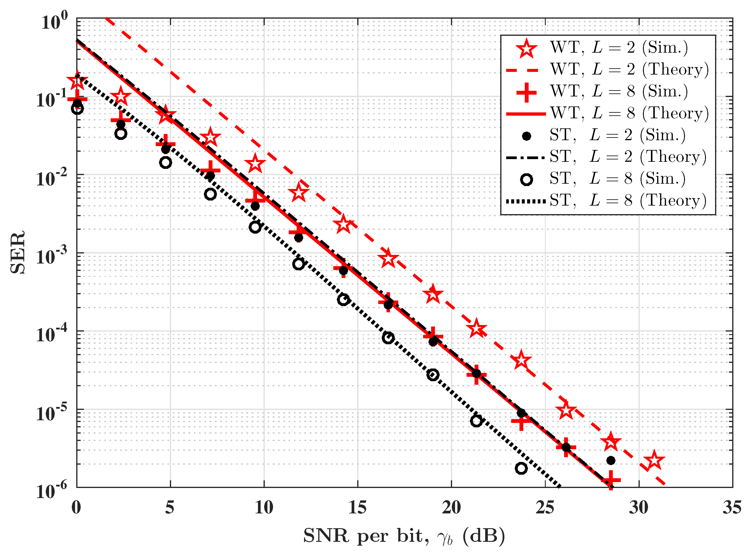
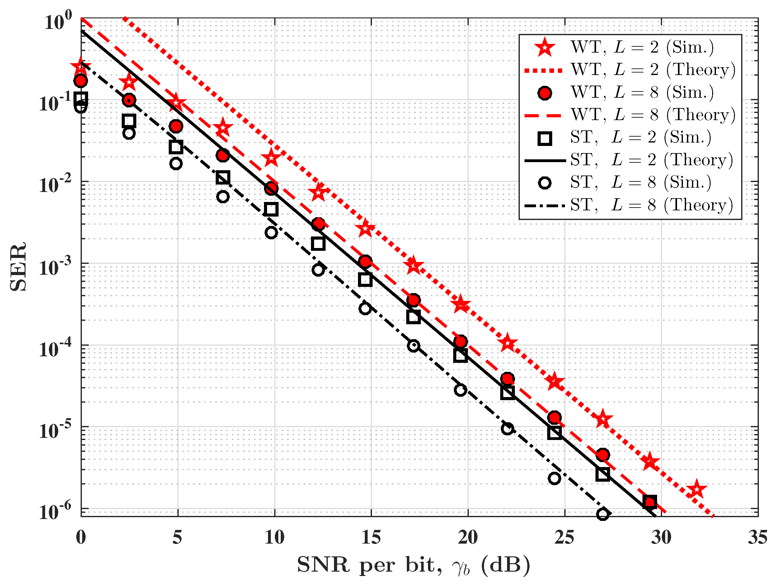
Without any loss of generality, considering the SPPM configuration with $N_{\mathrm{t}}=2$, $N_{\mathrm{r}}=4$, and $L=[2,8]$, the plots of the SER versus SNR per bit, ${\gamma }_{\mathrm{b}}$, under weak and strong AT conditions are shown in Figure 2. Similar error performance plots for the case of $N_{\mathrm{t}}=4$ are depicted in Figure 3. It can be observed from Figure 2 and Figure 3 that the derived upper bound on the asymptotic SER of SPPM in AT is closely matched by the simulation results. The error performance plot for moderate AT conditions is similar to that of the strong AT, and hence for clarity, the plot for moderate AT is not included. The reason for the SER values being greater than one, as well as the slight deviations observed between the theoretical and simulation results for SER $>{10}^{-2}$, is due to the union bound technique used in the analysis. Indeed, the closed form expression obtained in Section 3 can be used to study the performance of SPPM in outdoor Gamma-Gamma fading channels without performing computationally-intensive Monte Carlo simulations. In addition, using the PDF of the difference between two weighted GG RVs in Section 3, the framework can be extended to explore the performance of other variants of the OSM technique, such as spatial pulse amplitude modulation (SPAM) and generalised SPPM (GSPPM), in FSO channels. For instance, to extend the framework to study the SPAM scheme, PAM is used in place of the PPM scheme, and the transmit power weights, $\omega$, designed for creating power imbalance in this paper, will then represent the different intensity levels of the PAM scheme.

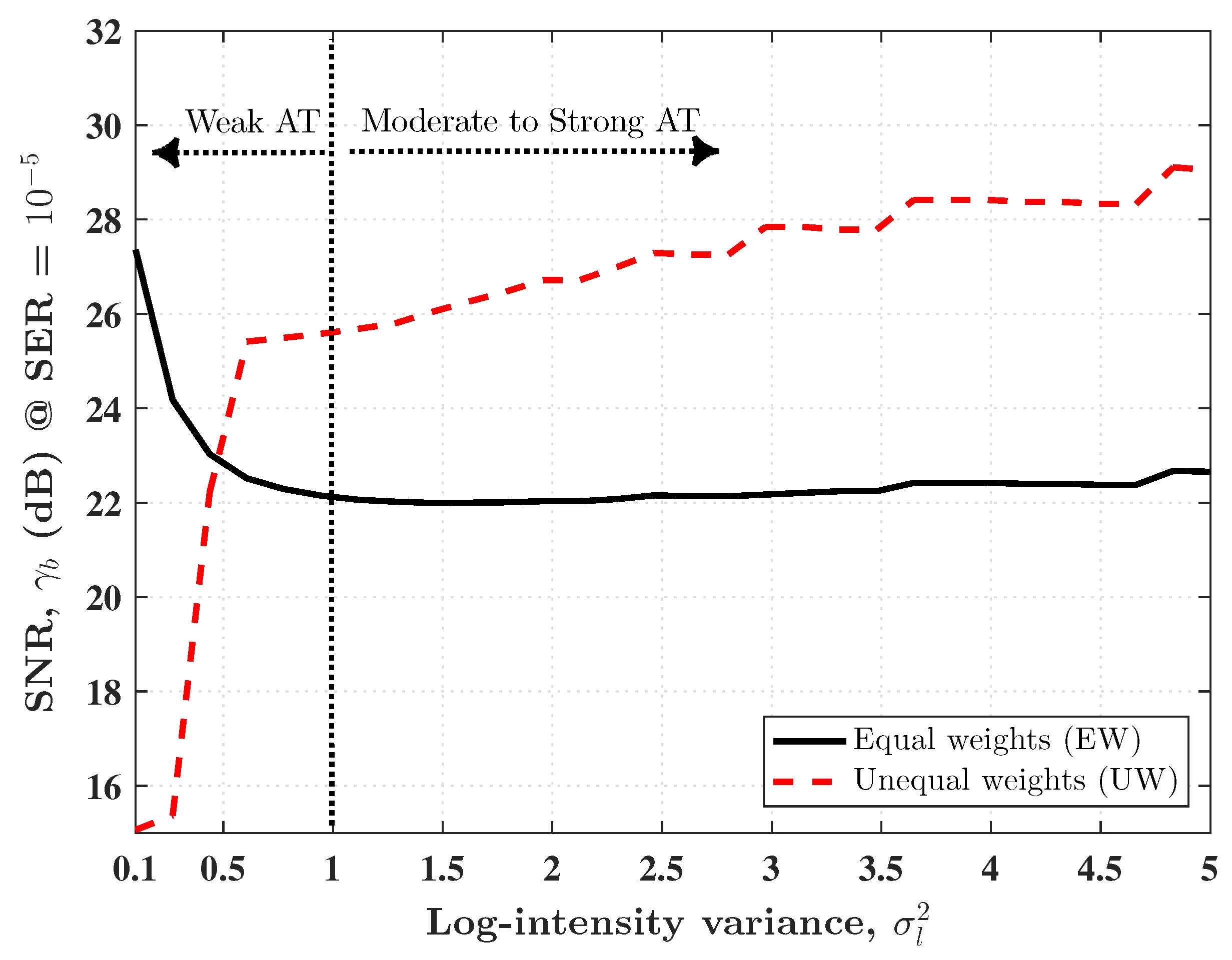
Using $N_{\mathrm{t}}=4$, $N_{\mathrm{r}}=4$, and $L=8$, the SNR required to achieve a representative SER of ${10}^{-5}$ under different AT regimes is depicted in Figure 4. For the case of equal transmit power weights, i.e., ${\left\{{\omega }_j\right\}}_{j=1}^{N_{\mathrm{t}}}=1$, it is observed that the SNR required under moderate-to-strong AT conditions is smaller compared to weak AT cases. As an example, under weak (${\sigma }_l^2=0.2$), moderate (${\sigma }_l^2=1.6$), and strong (${\sigma }_l^2=3.5$) AT regimes, the required SNR is about 24.5 dB, 22 dB, and 22.3 dB, respectively. This observation can be attributed to the fact that as the AT strength increases from weak to strong, the distribution of the fading coefficients spreads out more, and the range of possible values of the coefficients increases [1]. Since SPPM, like other OSM schemes, thrives on having distinct channel coefficients, then a better performance is expected under moderate-to-strong AT compared to weak AT. However, we also note that as the AT strength increases, the effective SNR of the received signal also decreases due to fading. This explains the slight increase in SNR requirements (albeit, less than $0.7$ dB) observed under strong AT compared to moderate AT. Typically, the error performance of OSM schemes is dependent on both the individual values of the channel coefficients, as well as the difference between them [17,26], as expressed by (16) and (9), respectively.

Furthermore, the system performance under weak AT conditions can be improved by applying unequal power allocation (PA) to make the TXs more distinguishable at the receiver. That is, the optical sources transmit at different peak powers. To keep the average optical power constant, total emitted power is re-distributed by reducing the power of some TXs and assigning the surplus optical power to the other TXs. The optical PA factor $\rho$, $0<\rho \le 1$, is used to generate the transmit power weights as [27]:

$${\omega }_j=N_{\mathrm{t}}\frac{{\rho }^{j-1}}{{\sum }_{j=1}^{N_{\mathrm{t}}}{\rho }^{j-1}}\mathrm{for}j=1,\dots ,N_{\mathrm{t}}.$$

(18)

When the TXs are arranged in ascending order of their weights, $\rho$ is the ratio of the smaller to the bigger weights assigned to a pair of consecutive TXs. The higher the value of $\rho$, the bigger the relative difference in the transmit power weights assigned to each TX. The value of $\rho$ that is applied is dependent on the severity of the channel gain similarity, as well as the received SNR of the transmitted digital signal modulation. As an example, for $N_{\mathrm{t}}=4$, by setting $\rho =1$, $\rho =0.5$, and $\rho =0.25$, we obtain the weights as ${\left\{{\omega }_j\right\}}_{j=1}^{N_{\mathrm{t}}}=[1,1,1,1]$, ${\left\{{\omega }_j\right\}}_{j=1}^{N_{\mathrm{t}}}=[2.13,1.07,0.53,0.27]$, and ${\left\{{\omega }_j\right\}}_{j=1}^{N_{\mathrm{t}}}=[3.01,0.75,0.19,0.05]$, respectively. Considering the case of $\rho =0.5$, Figure 4 shows that under weak AT (${\sigma }_l^2\le 0.5$), by using unequal weights, a reduction in the SNR requirement is achieved compared to using equal weights. However, since the total transmit power is kept constant, by applying the PA technique, the SNR values of signals with the smaller weights are further reduced in addition to the attenuation caused by AT. This effect can be seen in the performance deterioration observed for ${\sigma }_l^2>0.5$ in Figure 4. The unequal PA technique is largely effective when the channel coefficients are less distinct, as in weak AT. To achieve the best results, the relationship between PA and error performance must be optimised by considering the impact of the PA technique on the detection of the transmitter index and the transmitted digital signal modulation.

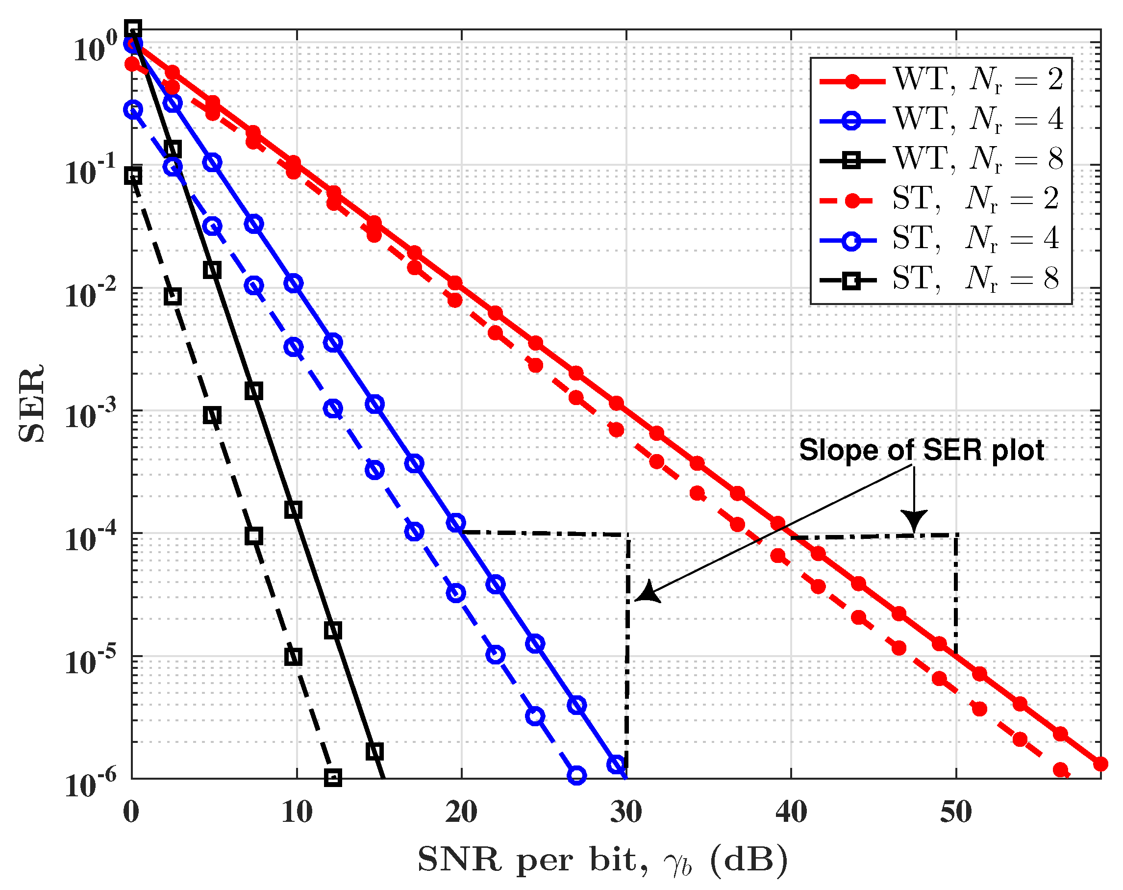
The SPPM scheme, as for OSM techniques in general, utilizes multiple optical sources at the transmitter to convey additional information bits, thereby providing increased throughput. Therefore, to achieve diversity gain, particularly in the dynamic FSO channels, multiple PDs can be employed at the receiver. Considering an SPPM configuration with $N_{\mathrm{t}}=4$ and $L=8$, the plots of SER against ${\gamma }_{\mathrm{b}}$ with multiple PD, under weak and strong AT conditions, are provided in Figure 5. As observed in Figure 5, as the number of PDs increases, the SNR required to attain a specified SER reduces across all the turbulence regimes. For example, under strong AT conditions, the SNR required to attain an SER of ${10}^{-5}$ is reduced by a factor of about 24 dB (from 46 dB to 22 dB) when the number of PDs is increased from two to four. In fact, the diversity order, obtained from the asymptotic slope of the SER curve (in log-log scale) in the high SNR regime [28], is $d_o=N_{\mathrm{r}}/2$, under all AT conditions. For instance, in Figure 5, under weak AT conditions, for $N_{\mathrm{r}}=2$, the SER at SNRs of 40 dB and 50 dB is ${10}^{-4}$ and ${10}^{-5}$, respectively. Thus, $d_o=-\log ({10}^{-5}/{10}^{-4})/\log ({10}^5/{10}^4)=1$. Furthermore, for $N_{\mathrm{r}}=4$, the SER at SNRs of 20 dB and 30 dB is ${10}^{-4}$ and ${10}^{-6}$, respectively, and $d_o=-\log ({10}^{-6}/{10}^{-4})/\log ({10}^3/{10}^2)=2$. Note that in computing the values of $d_o$, the SNR values have been converted from the decibel scale to the linear scale. Similar results can be obtained from the other error performance plots in Figure 5. Using multiple PDs improves the robustness of the SPPM system to turbulence-induced channel fading.

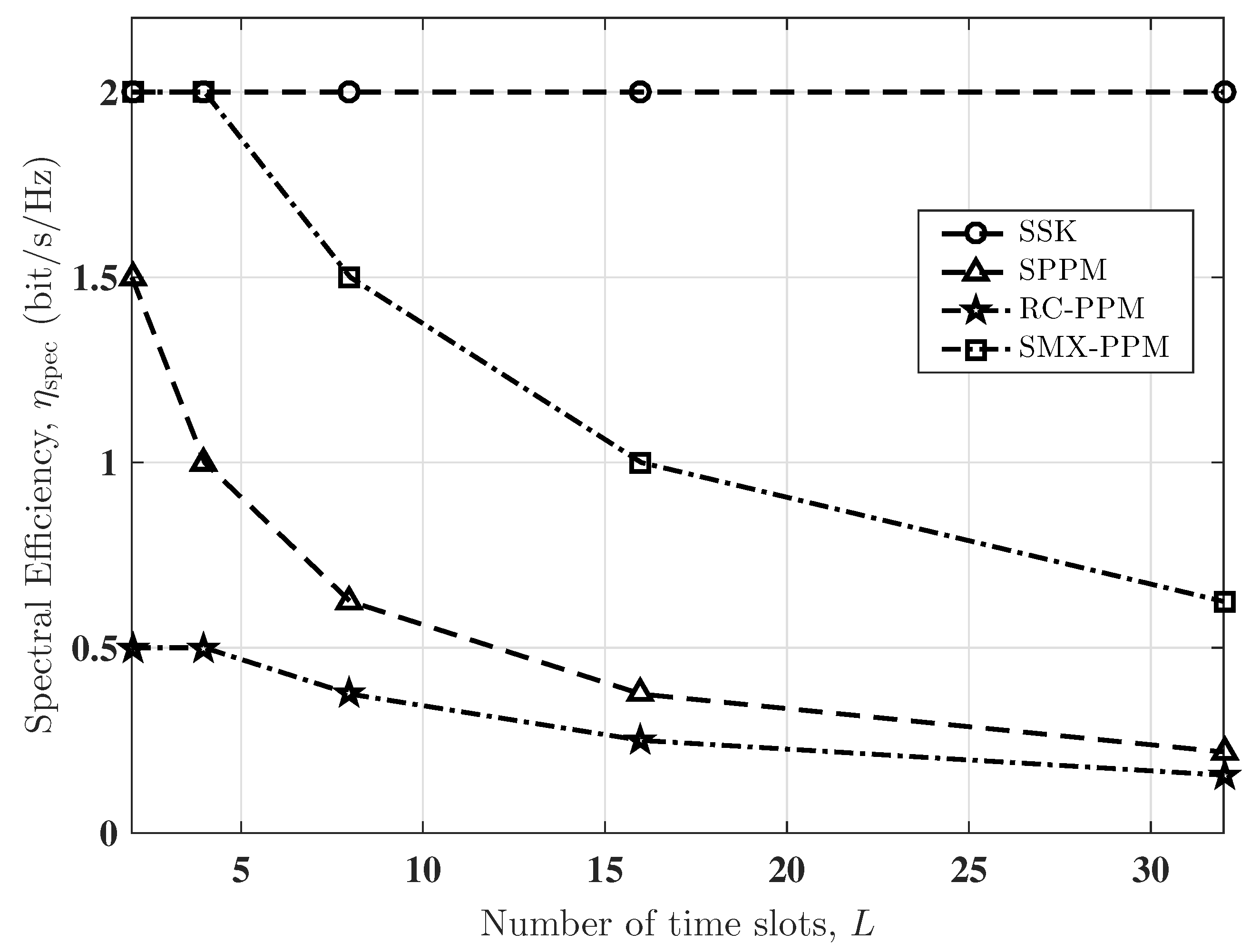
The performance comparison of SPPM with other MIMO schemes in terms of energy and spectral efficiencies is illustrated in Figure 6 and Figure 7, respectively. The SPPM is compared with SSK, repetition coded PPM (RC-PPM), and spatial multiplexed PPM (SMX-PPM) schemes. Spectral efficiency, ${\eta }_{\mathrm{spec}}$, is defined as the ratio of bit rate to the bandwidth requirement, where the bandwidth requirement is the reciprocal of pulse duration. For an energy efficiency comparison, we estimate the SNR required to achieve an SER of ${10}^{-5}$ using $N_{\mathrm{t}}=4$ and the same average transmitted optical power for all techniques. Figure 6 shows that the maximum spectral efficiency, ${\eta }_{\mathrm{spec}}$, of SPPM (using $L=2$) exceeds that of RC-PPM by 1 bit/s/Hz. This is due to the increase in the number of bits transmitted per symbol in SPPM by encoding additional information on the spatial index of the TX. The value of ${\eta }_{\mathrm{spec}}$ is higher for SSK compared to SPPM because the pulse duration in SSK is L-times longer than that of SPPM, though SPPM transmits more bits/symbol. 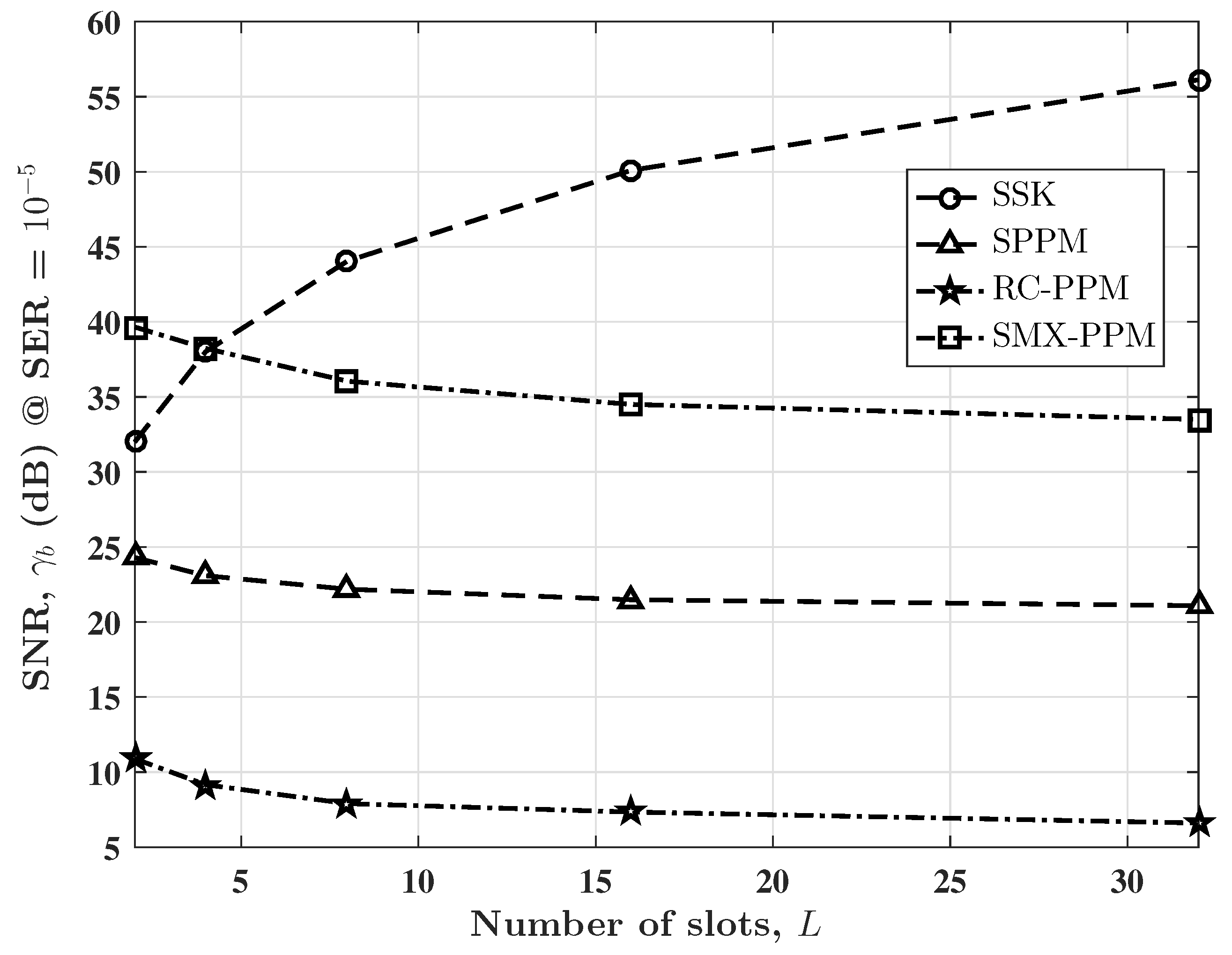As expected, due to the multiplexing gains of SMX-PPM, its ${\eta }_{\mathrm{spec}}$ is higher than that of SPPM. However, as shown in Figure 7, the SPPM scheme achieves up to 15.4 dB (using $L=2$) of savings in SNR compared to SMX-PPM. This is because, in SPPM, only one TX is activated in a given symbol duration, whereas, for SMX-PPM, all the TXs are activated concurrently, and their emitted intensities are divided by a factor of $N_{\mathrm{t}}$ in order to achieve equal average transmitted optical power. Moreover, the single-transmitter activation in SPPM prevents interchannel interference, which reduces the complexity of the detection algorithms. Compared to SSK, the SPPM schemes achieve up 35 dB of savings in SNR due to the use of PPM, which gives a shorter pulse duration. As L increases, the energy savings by SPPM, in terms of SNR, increase. This highlights how the power efficiency benefits of PPM are harnessed in SPPM. These results therefore show clearly how the SPPM combines the energy efficiency of the PPM with the high spectral efficiency and low complexity of SM to provide an attractive performance trade-off. This permits a flexible implementation based on the data rate and error performance requirements of the target application. For instance, in wireless sensor networks, which are constrained by energy resource and processing capacity, SPPM with its low complexity, energy efficiency, and improved spectral efficiency (over PPM) is a viable technique.

5. Conclusions

The theoretical upper bound on the asymptotic SER for SPPM based an FSO system has been presented in different atmospheric turbulence regimes from weak to strong. The turbulence-induced fading in the FSO channel is modelled by the widely-adopted Gamma-Gamma distribution. Our analytical framework provides a closed-form expression for the SER, and it can be extended to explore the performance of other OSM schemes in FSO channels. Error performance plots show that SPPM is viable even in strong turbulence conditions. The spread of the fading coefficients increases with the turbulence strength. This implies that the level of the differentiability of the channel is higher in strong turbulence. Thus, a better error performance is observed under moderate-to-strong AT compared to weak AT. The performance in weak AT can however be improved by applying unequal transmit power allocation to make the FSO links more identifiable at the receiver. Spatial diversity has been considered at the receiver to mitigate irradiance fluctuation and improve the robustness of the SPPM-FSO system to channel fading. The diversity order is obtained as half of the number of detectors employed at the receiver. In terms of energy and spectral efficiencies, the performance of SPPM is compared with conventional MIMO techniques such as repetition coding and spatial multiplexing. Future work will be to apply the framework presented in this paper in exploring the performance of other variants of the OSM technique in FSO, particularly the generalised OSM scheme.

References

1. Ghassemlooy, Z.; Popoola, W.; Rajbhandari, S. Optical Wireless Communications: System and Channel Modelling with Matlab®; CRC Press, Inc.: Boca Raton, FL, USA, 2012. [Google Scholar]
2. Khalighi, M.A.; Uysal, M. Survey on Free Space Optical Communication: A Communication Theory Perspective. IEEE Commun. Surv. Tutor. 2014, 16, 2231–2258. [Google Scholar] [CrossRef]
3. Gappmair, W.; Hranilovic, S.; Leitgeb, E. Performance of PPM on Terrestrial FSO Links with Turbulence and Pointing Errors. IEEE Commun. Lett. 2010, 14. [Google Scholar] [CrossRef]
4. Bayaki, E.; Schober, R.; Mallik, R.K. Performance Analysis of MIMO Free-Space Optical Systems in Gamma-Gamma Fading. IEEE Trans. Commun. 2009, 57, 3415–3424. [Google Scholar] [CrossRef]
5. Popoola, W.O.; Ghassemlooy, Z. BPSK Subcarrier Intensity Modulated Free-Space Optical Communications in Atmospheric Turbulence. J. Lightw. Technol. 2009, 27, 967–973. [Google Scholar] [CrossRef] [Green Version]
6. Bhatnagar, M.R.; Ghassemlooy, Z. Performance Analysis of Gamma-Gamma Fading FSO MIMO Links With Pointing Errors. J. Lightw. Technol. 2016, 34, 2158–2169. [Google Scholar] [CrossRef]
7. Song, X.; Cheng, J. Subcarrier Intensity Modulated MIMO Optical Communications in Atmospheric Turbulence. J. Opt. Commun. Netw. 2013, 5, 1001–1009. [Google Scholar] [CrossRef]
8. Mesleh, R.Y.; Haas, H.; Sinanovic, S.; Ahn, C.W.; Yun, S. Spatial Modulation. IEEE Trans. Veh. Technol. 2008, 57, 2228–2241. [Google Scholar] [CrossRef]
9. Mesleh, R.; Elgala, H.; Haas, H. Optical Spatial Modulation. IEEE/OSA J. Opt. Commun. Netw. 2011, 3, 234–244. [Google Scholar] [CrossRef]
10. Jaiswal, A.; Bhatnagar, M.R.; Jain, V.K. Performance Evaluation of Space Shift Keying in Free-Space Optical Communication. IEEE/OSA J. Opt. Commun. Netw. 2017, 9, 149–160. [Google Scholar] [CrossRef]
11. Abaza, M.; Mesleh, R.; Mansour, A. Performance Analysis of Space-Shift Keying over Negative-Exponential and Log-Normal FSO Channels. Chin. Opt. Lett. 2015, 13, 051001. [Google Scholar] [CrossRef]
12. Jaiswal, A.; Bhatnagar, M.R.; Jain, V.K. BER Analysis of Optical Space Shift Keying in Atmospheric Turbulence Environment. In Proceedings of the 2016 10th International Symposium on Communication Systems, Networks and Digital Signal Processing (CSNDSP), Prague, Czech Republic, 20–22 July 2016; pp. 1–6. [Google Scholar]
13. Özbilgin, T.; Koca, M. Optical Spatial Modulation Over Atmospheric Turbulence Channels. J. Lightw. Technol. 2015, 33, 2313–2323. [Google Scholar] [CrossRef]
14. Peppas, K.P.; Mathiopoulos, P.T. Free-Space Optical Communication With Spatial Modulation and Coherent Detection Over H-K Atmospheric Turbulence Channels. J. Lightw. Technol. 2015, 33, 4221–4232. [Google Scholar] [CrossRef]
15. Jaiswal, A.; Bhatnagar, M.R.; Jain, V.K. Performance of Optical Space Shift Keying Over Gamma–Gamma Fading With Pointing Error. IEEE Photonics J. 2017, 9, 1–16. [Google Scholar] [CrossRef]
16. Odeyemi, K.O.; Owolawi, P.A.; Srivastava, V.M. Optical spatial modulation over Gamma–Gamma turbulence and pointing error induced fading channels. Opt. Int. J. Light Electron. Opt. 2017, 147, 214–223. [Google Scholar] [CrossRef]
17. Popoola, W.O.; Poves, E.; Haas, H. Spatial Pulse Position Modulation for Optical Communications. J. Lightw. Technol. 2012, 30, 2948–2954. [Google Scholar] [CrossRef]
18. Andrews, L.C.; Phillips, R.L. Laser Beam Propagation Through Random Media; SPIE Press: Bellingham, WA, USA, 2005. [Google Scholar]
19. Olanrewaju, H.G.; Thompson, J.; Popoola, W.O. Performance of Optical Spatial Modulation in Indoor Multipath Channel. IEEE Trans. Wirel. Commun. 2018, 17, 6042–6052. [Google Scholar] [CrossRef]
20. Kahn, J.M.; Barry, J.R. Wireless Infrared Communications. Proc. IEEE 1997, 85, 265–298. [Google Scholar] [CrossRef]
21. Andrews, L.C.; Phillips, R.L.; Hopen, C.Y. Laser Beam Scintillation with Applications; SPIE Press: Bellingham, WA, USA, 2001; Volume 99. [Google Scholar]
22. Prudnikov, A.P.; Brychkov, Y.A.; Marichev, O.I. Integrals and Series, Volume 3: More Special Functions; Gordon and Breach: Philadelphia, PA, USA, 1990; Volume 3. [Google Scholar]
23. Osche, G.R. Optical Detection Theory for Laser Applications; Wiley: Hoboken, NJ, USA, 2002. [Google Scholar]
24. Ng, E.W.; Geller, M. A Table of Integrals of the Error Function. J. Res. Natl. Bur. Stand. 1968, 73B, 149–163. [Google Scholar] [CrossRef]
25. Proakis, J.; Salehi, M. Digital Communications, 5th ed.; McGraw-Hill: New York, NY, USA, 2008. [Google Scholar]
26. Zhang, X.; Dimitrov, S.; Sinanovic, S.; Haas, H. Optimal Power Allocation in Spatial Modulation OFDM for Visible Light Communications. In Proceedings of the 2012 IEEE 75th Vehicular Technology Conference (VTC Spring), Yokohama, Japan, 6–9 May 2012; pp. 1–5. [Google Scholar]
27. Fath, T.; Haas, H. Performance Comparison of MIMO techniques for Optical Wireless Communications in Indoor Environments. IEEE Trans. Commun. 2013, 61, 733–742. [Google Scholar] [CrossRef]
28. Lozano, A.; Jindal, N. Transmit diversity vs. spatial multiplexing in modern MIMO systems. IEEE Trans. Wirel. Commun. 2010, 9, 186–197. [Google Scholar] [CrossRef] [Green Version]
29. Chiani, M.; Dardari, D.; Simon, M.K. New Exponential Bounds and Approximations for the Computation of Error Probability in Fading Channels. IEEE Trans. Wirel. Commun. 2003, 2, 840–845. [Google Scholar] [CrossRef]
Figure 1. Illustration of spatial pulse position modulation (SPPM) encoding using N t = 4 , L = 4 .
Photonics 05 00053 g001
Figure 2. Error performance of SPPM in weak and strong atmospheric turbulence (AT) conditions. N t = 2 , N r = 4 , and L = [ 2 , 8 ] . ST, strong AT; WT, weak AT; SER, symbol error rate.
Photonics 05 00053 g002
Figure 3. Error performance of SPPM in weak and strong AT conditions. N t = 4 , N r = 4 , and L = [ 2 , 8 ] .
Photonics 05 00053 g003
Figure 4. Performance under a varying AT regime. SNR required to achieve SER of 10 5 for the SPPM configuration: N t = 4 , L = 8 .
Photonics 05 00053 g004
Figure 5. SNR required to achieve SER = 10 5 , using varying numbers of photodetectors (PDs). SPPM configuration: N t = 4 , L = 8 .
Photonics 05 00053 g005
Figure 6. Spectral efficiency comparison of SPPM with space shift keying (SSK), repetition coding (RC)-PPM, and spatial multiplexing (SMX)-PPM for different values of L, using N t = 4 , and under the strong AT condition.
Photonics 05 00053 g006
Figure 7. Energy efficiency comparison of SPPM with SSK, RC-PPM, and SMX-PPM for different values of L, using N t = 4 , N r = 4 , and under the strong AT condition.
Photonics 05 00053 g007