
Coping with the Inequity and Inefficiency of the H-Index: A Cross-Disciplinary Empirical Analysis


1
Dipartimento di Scienze per la Qualità della Vita, Università di Bologna, C.so d’Augusto 237, 47921 Rimini, Italy
2
Dipartimento di Scienze Statistiche “Paolo Fortunati”, Università di Bologna, 40126 Bologna, Italy
*
Author to whom correspondence should be addressed.
Publications 2024, 12(2), 12; https://doi.org/10.3390/publications12020012
Submission received: 3 November 2023
/
Revised: 10 April 2024
/
Accepted: 15 April 2024
/
Published: 22 April 2024
Abstract
:This paper measures two main inefficiency features (many publications other than articles; many co-authors’ reciprocal citations) and two main inequity features (more co-authors in some disciplines; more citations for authors with more experience). It constructs a representative dataset based on a cross-disciplinary balanced sample (10,000 authors with at least one publication indexed in Scopus from 2006 to 2015). It estimates to what extent four additional improvements of the H-index as top-down regulations (∆Hh = Hh − Hh+1 from H1 = based on publications to H5 = net per-capita per-year based on articles) account for inefficiency and inequity across twenty-five disciplines and four subjects. Linear regressions and ANOVA results show that the single improvements of the H-index considerably and decreasingly explain the inefficiency and inequity features but make these vaguely comparable across disciplines and subjects, while the overall improvement of the H-index (H1–H5) marginally explains these features but make disciplines and subjects clearly comparable, to a greater extent across subjects than disciplines. Fitting a Gamma distribution to H5 for each discipline and subject by maximum likelihood shows that the estimated probability densities and the percentages of authors characterised by H5 ≥ 1 to H5 ≥ 3 are different across disciplines but similar across subjects.
1. Introduction
To the best of our knowledge, few papers (e.g., [1,2]) suggest an index to evaluate interdisciplinary CVs (i.e., authors applying usual methodologies to unusual topics or vice versa). In particular, Zagonari [1] identifies the interdisciplinary percentage of any CV (i.e., articles in a discipline or subject quoted by articles in different disciplines or subjects) to be applied to the H-index characterising each author, where the H-index is chosen as an easily generated quantitative index. However, this interdisciplinary index requires a homogeneous H-index across disciplines or subjects to avoid gains for some interdisciplinary scientists (e.g., across medicine and computing) and losses for other interdisciplinary scientists (e.g., across art and mathematics) [3].
Within the huge theoretical and empirical literature on variants and extensions of the H-index (e.g., a-index, ar-index, m-quotient, raw h-rate, contemporary h-index, f-index, t-index, wu-index, maxpord index, q2-index within variants, and hw-index, hm-index, hi-index, hc-index, m-quotient, ht-index, fraction count on citation, fraction count on paper, age-based h-index) [4,5,6], some papers suggest some improvements of the H-index to increase homogeneity across disciplines (e.g., [7,8,9,10]). In particular, Zagonari [9] develops an empirically validated theoretical model of a researcher’s publication goal by providing two internal criteria (i.e., efficiency and equity) to evaluate a bibliometric index (i.e., it grounds these concepts on an analytical model representing the researchers’ incentives to maximise their H-index) and by suggesting two standardisations (i.e., calculate publications per author and citations per author per year) and two guidelines (i.e., neglect co-authors’ reciprocal citations and publications other than peer-reviewed articles) to predict which standardisations and guidelines are most likely to succeed in achieving efficiency and equity across disciplines. The following relationships between improvements, criteria, standardisations, and guidelines are identified:
- Inefficiency (i.e., biased incentives to the research activity in terms of scientific achievements) is managed by focusing on articles instead of publications (i.e., publications include non-peer reviewed research) (Inefficiency a, Ifa hereafter) and by using net instead of gross citations (i.e., gross citations include co-authors’ reciprocal citations) (Inefficiency b, Ifb hereafter). In terms of H-index improvements, ∆H1 = H1 − H2 deals with the overvaluation of possibly non-original research such as reviews, proceedings, and editorials, where H1 = H-index based on publications and H2 = H-index based on articles; ∆H2 = H2 − H3 deals with the overemphasis put on co-authors’ reciprocal citations as a measure of actual knowledge diffusion, where H3 = H-index based on net citations for articles.
- Inequity (i.e., biased rankings in favour of some authors and some disciplines) is managed by using a per-capita H-index to account for the different co-authorship practices prevailing in different disciplines (i.e., more co-authors in some disciplines) (Inequity a, Iqa hereafter) and by using a per-year H-index to account for the different citation periods related to authors with more scientific experience (i.e., they can rely on a longer citation period) (Inequity b, Iqb hereafter). In terms of H-index improvements, ∆H3 = H3 − H4 deals with the huge differences in the number of co-authors and thus in the number of articles in favour of some disciplines, where H4 = net per-capita H-index based on articles; ∆H4 = H4 − H5 deals with the obviously large number of citations received by researchers with more experience and thus the likely worse assessment of the scientific production in disfavour of researchers with less experience, where H5 = net per-capita per-year H-index based on articles.
Note that all acronyms and variables are described in Table 1. Zagonari [9] is focused on the degree of efficiency and equity rather than on the homogeneity across disciplines which can be achieved by the suggested standardisations and guidelines, and a theoretical approach is adopted (although the structural model is validated in terms of means and variances) rather than a statistical approach (where reduced models are tested in terms of residuals and distributions). Note that Ifa favours authors who minimise efforts and risks related to a collaborative and creative scientific activity by relying on the large number of citations to reviews. Ifb favours authors who spend efforts on networking at no risk rather than on a creative scientific activity. Iqa favours authors who reduce efforts and risks (i.e., they misuse the prevailing measurement of scientific activity based on the principle “one article with n co-authors is n articles”), by spending efforts on networking rather than on a creative scientific activity. Iqb favours authors who minimise efforts at no risk (i.e., they misuse the prevailing measurement of scientific activity based on the principle “the overall sum of citations matters”) by spending efforts on networking rather than on a creative scientific activity.
Within the recent empirical literature on indexes for interdisciplinary science (e.g., [11]), the purpose of this paper is to statistically test to what extent the suggested improvements of the H-indexes [9], considered as top-down regulations, account for different publication and citation habits characterising different disciplines and subjects in order to enable suitable comparisons of interdisciplinary scientists [1] across disciplines and subjects. To do so, we suggest some measures of inefficiency and inequity in Section 2. We construct a representative sample in Section 3. We provide results for each single H-index improvement ∆Hh based on linear regressions and analysis of variance (ANOVA) in Section 4.1 as well as results for H5 based on maximum likelihood fittings and quantile analysis in Section 4.2 by introducing the assumption that the observed H5 values for both disciplines and subjects are realisations of a gamma distribution. This is followed by a discussion of findings, weaknesses, and strengths in Section 5, before conclusions and final remarks about methodological and practical potentials in Section 6.
Note that the use of H-index improvements suggested by Zagonari [9] instead of other developments will be justified in Section 5. Moreover, our observation unit will be each author (Ai), rather than journals (e.g., [12]) or institutions (e.g., [13]), since our goal is the evaluation of interdisciplinary scientists. Finally, the use of H-index improvements as policies suggested by Zagonari [9] will be justified in Section 6.
In other words, the research questions of the present study can be summarised as follows:
- Does each single H-index improvement ∆Hh properly solve inefficiency and inequity issues?
- Does each single H-index improvement ∆Hh spread inefficiency and inequity issues uniformly across disciplines Dj and subjects Sk?
- Can any discipline Dj and subject Sk be distinguished from other disciplines and subjects, respectively, net of ∆Hh?
- Does the comprehensive H-index improvement H1–H5 properly solve inefficiency and inequity issues?
- Does the comprehensive H-index improvement H1–H5 spread inefficiency and inequity issues uniformly across disciplines Dj and subjects Sk?
- Can any discipline Dj and subject Sk be distinguished from other disciplines and subjects, respectively, net of H1–H5?
- Are disciplines Dj and subjects Sk characterised by similar parametric distributions for H5 (i.e., plots have similar shapes) and by similar right tails (i.e., similar percentages of authors with H5 ≥ 1, H5 ≥ 1.5, H5 ≥ 2, H5 ≥ 2.5, H5 ≥ 3)?
Note that improvements of H-indexes are taken as policies based on limited information about each single author (e.g., year of the first publication) or discipline and subject (e.g., average number of citations per article). Moreover, the application of the interdisciplinary index to a homogeneous H-index refers to subjects to a greater extent than disciplines (i.e., really powerful interdisciplinary research is across subjects). Statistical analyses of this feature are presented for subjects in the Results and for disciplines in the Appendix A, Appendix B, Appendix C and Appendix D. Finally, as for a classification of studies on bibliometrics in terms of internal vs. external criteria (e.g., [14]) and in terms of theoretical vs. empirical approaches (e.g., [15]), the present paper refers to external theoretical concepts (i.e., efficiency and equity, by adding the concept of homogeneity across disciplines), but it adopts an empirical approach. This feature implies that our results will depend on the used sample: in other words, a theoretical proof based on internal criteria will not be attained, similarly to all other empirical studies. However, we will refer to external criteria of judgment supported by the structural model validated in Zagonari [9] and we will perform a statistical analysis of reduced forms of the same model by referring to the same dataset used in Zagonari [9].
In summary, by focusing on subjects Sk, apart from ∆H2, neither each single H-index improvement nor the comprehensive H-index improvement solves inefficiency and equity issues (i.e., answer NO to research questions 1 and 4), although the comprehensive H-index improvement makes them confidently uniform across subjects (i.e., answer NO to research question 2 and answer YES to research question 5). Moreover, apart from subject S1 for Ifa and subject S4 for Ifb, all subjects are similar in terms of inefficiency and inequity (i.e., answer NO to research question 3 and answer NO to research question 6). Finally, subjects show similar gamma distribution fits and similar right tails (i.e., answer YES to research question 7).
2. Measuring Inefficiency and Inequity by H-Indexes
In order to check if improved H-indexes solve efficiency and equity problems on average and to a greater or smaller extent in each single discipline, efficiency and equity and H improvements described in Section 1 are specified as follows (i.e., Npub = number of publications, Nart = number of articles, Ngro = number of citations including co-author citations, Nnet = number of citations excluding co-author citations, Naut = mean number of co-authors for each author, expert = authors with the first publication before 2011 to include up to 10 years from 2006 to 2015, inexpert = authors with the first publication after 2010 to include up to 5 years from 2006 to 2010):
- Inefficiency a (i.e., many publications other than articles for each author):
- Inefficiency b (i.e., many co-authors’ reciprocal citations for each author):
- Inequity a (i.e., more co-authors in some disciplines):
- Inequity b (i.e., more citations for authors with more experience):
Note that Npub is likely to be underestimated, since many reviews are published as articles. Moreover, estimations are based on differences if the bias under consideration affects the number of citations only (i.e., Equations (2) and (4)) as well as if the bias affects both the number of authors and the number of citations (i.e., Equations (1) and (3)). Finally, each subsequent bias is additional to the previous one. Thus, in order to test the performances of the comprehensive H-index improvement for addressing the overall bias, we will refer to the following equation:
where the lhs represents the overall bias, since the focus is on publications for expert authors and on articles for inexpert authors. We will perform similar analyses for subjects by replacing the dummy variables for disciplines Dj with the dummy variables for subjects Sk.
Note that Zagonari [9] does not include H4 and H5. Moreover, Zagonari [1] shows that interdisciplinary science requires an additional category, together with orthodox science (i.e., authors publish in a single discipline and in many journals, and the vast majority of the citations are in few disciplines but in many different journals) and heterodox science (i.e., authors publish in a single discipline and in a few journals devoted to that discipline, so that the vast majority of citations are in few disciplines and few journals), to be combined with H5 to reduce unfair rankings between interdisciplinary scientists (i.e., authors publish in many disciplines and journals, and the vast majority of citations are in many different disciplines and journals) across different disciplines as well as between interdisciplinary scientists and single-discipline scientists collaborating with many authors from different disciplines. Finally, Zagonari [9] does not include quantitative results based on linear regressions or parameter estimations.
3. Constructing the Dataset
In order to obtain a representative dataset for authors, we applied the following stratified sampling. The reference population consists of authors with at least one publication in the Scopus dataset from 2006 to 2015. This population is partitioned by discipline: we used the 27 scientific disciplines suggested by Scopus [16].
By preserving the percentages of authors in each scientific discipline, 10,000 authors are then randomly extracted from the Scopus database. This design required the attribution of each author to a single discipline: we used the attribution suggested by Scopus, where an author is linked to the discipline with the largest percentage of publications.
Table 2 and Table 3 provide the summary statistics for subjects Sk, while Appendix B provides the summary statistics for disciplines Dj. Altogether, the dataset includes 1,487,866 co-authors, 507,557 papers, 31,950 journals, and 562,688 citations. The Supplementary Materials provide the histograms of H1 and H5 for both disciplines Dj and subjects Sk.
4. Results
4.1. ANOVA and Linear Regressions
In order to check if the improved H-indexes solve efficiency and equity problems on average and to a greater or smaller extent in each discipline, we will perform ANOVA based on linear regressions [17] (see Appendix D for ANOVA based on a quasi-Poisson distribution). In particular, we will translate the theoretical models presented in Section 2 into regression models as follows (i.e., Aaut takes value 1 for authors with the first publication after 2010):
- Inefficiency a (i.e., many publications other than articles for each author):
- Inefficiency b (i.e., many co-authors’ reciprocal citations for each author):
- Inequity a (i.e., more co-authors in some disciplines):
- Inequity b (i.e., more citations for authors with more experience):
Note that we disregarded discipline #10 (multidisciplinary) and discipline #36 (health professions), since few authors are attached to them in our sample (i.e., 2 authors for discipline #10 and 1 author for discipline #36). Moreover, in the model for Iqa (i.e., Equation (8)), Naut is moved to the rhs. Indeed, this inequity is based on the prediction that authors with several co-authors are likely to achieve more citations (i.e., Naut is a stochastic variable). We estimated this relationship before trying to explain the impact of this H-index improvement on rhs and check for residual heterogeneity explained by the discipline dummies. Finally, in the model for Iqb (i.e., Equation (9)), both Naut and Aaut are moved to the rhs. Indeed, this inequity is based on the prediction that expert authors with several co-authors are likely to achieve more citations (i.e., Naut and Aaut are stochastic variables). Again, we estimated these relationships before trying to explain the impact of this H-index improvement on rhs and check for residual heterogeneity explained by the discipline dummies. Thus, the overall bias can be represented by:
where the focus is on articles. We will perform similar analyses for subjects Sk.
Note that we will check firstly for the significance levels of variables and secondly for their coefficient values. Moreover, Equation (10) can be obtained by summing up terms of rhs and lhs in Equations (6)–(9). Finally, we will check for differences between specific disciplines or subjects only if their general explanation of variability is significant.
A methodological remark is worth making here. An ANOVA exercise as a descriptive method (i.e., calculated significance levels) relies on the assumption of normal distributions, although its descriptive statistics (i.e., estimated coefficients and explained variance) allows a simple interpretation of results. Each ANOVA table in Section 4.1 is associated with an analogous table in Appendix D based on a log-linear model involving Poisson and negative-binomial distributions; additional methodological details are provided in Appendix D.
4.1.1. Inefficiency a (Ifa) (Many Publications Other Than Articles)
All authors in our dataset have H1 = H2 (i.e., ∆H1 does not affect Inefficiency a). In other words, publications other than articles do not affect their H-index (e.g., eminent authors are asked to write a review or a book). Consequently, we will apply ANOVA only to disciplines and subjects. In particular, Table 4 shows that the variance explained by disciplines Dj is mildly significant but tiny. In contrast, Table 5 shows that the variance explained by subjects Sk is significant but tiny. Note that we will hereafter use slightly significant whenever * applies (i.e., significant at 95%), mildly significant whenever ** applies (i.e., significant at 99%), and significant whenever *** applies (i.e., significant at 99.9%).
Next, Table A4 in Appendix C shows that, apart from D27 and D35, all disciplines Dj are characterised by a percentage of publications other than articles smaller than 1. Similarly, Table 6 shows that, apart from S1, all subjects Sk are characterised by a percentage of publications other than articles smaller than 1.
4.1.2. Inefficiency b (Ifb) (Many Co-Authors’ Reciprocal Citations)
The application of ANOVA to Ifb (i.e., Equation (7)) shows that ∆H2 explains 26.79% of its variability. In particular, Table 7 and Table 8 show that the residual variances explained by disciplines Dj and subjects Sk are slightly significant and tiny (i.e., ∆H2 makes Dj and Sk homogeneous with respect to Ifb). In other words, 26.79% of the Ifb variability is explained by ∆H2. The remaining 73.21% of its variability can be decomposed in variance between disciplines in Table 7 (subjects in Table 8) that accounts for only 0.29% (0.06% in Table 8) and variance within disciplines (subjects) that accounts for the remaining 72.92% (73.15% in Table 8). Thus, even if disciplines and subjects are slightly significant, these factors explain very little of Ifb (i.e., we can safely affirm that, once the Ifb variability explained by ∆H2 is removed, the remaining variance is within disciplines and subjects to a greater extent than across disciplines and subjects: 72.92% > 0.29%).
Next, Table A5 in Appendix C shows that, apart from D13, D27, and D31, all disciplines Dj are characterised by an insignificant intercept in the linear regression (7) (i.e., ∆H2 depicts intercepts for those disciplines), where two significant coefficients are positive and large (i.e., larger than 0.1). Similarly, Table 9 shows that, apart from S4, all subjects Sk are characterised by a significant and positive intercept in the linear regression (7) (i.e., ∆H2 depicts intercepts only for that subject), where one significant coefficient is positive and tiny (i.e., larger than 0.1).
Note that we did not detail comparisons between subjects and disciplines, since the variance explained by subjects and disciplines altogether is slightly significant and tiny.
4.1.3. Inequity a (Iqa) (More Co-Authors in Some Disciplines)
The application of ANOVA to Iqa (i.e., Equation (8)) shows that ∆H3 describes 4.38% of its variability. In particular, Table 10 shows that the variance explained by disciplines Dj is significant and small (i.e., ∆H3 does not make Iqa homogeneous across disciplines Dj). In contrast, Table 11 shows that the variance explained by subjects Sk is significant and tiny (i.e., ∆H3 makes Iqa homogeneous across subjects Sk).
Note that Table 12 for subjects and Table A6 in Appendix C for disciplines suggest that adding one co-author to an author significantly affects the number of net citations by around 0.01. In other words, Iqa, although it is statistically significant, it turns out to be a marginal feature for most authors (i.e., to have a substantial effect on the number of citations, an author should publish with several hundreds or thousands of co-authors). However, ∆H3 contains more information than the number of authors to explain the number of net citations, both for subjects (i.e., 1.68 > 0.0097) and disciplines (i.e., 1.61 > 0.0105).
Next, Table A6 in Appendix C shows that, apart from D12, D18, D20, D21, D26, D29, D30, D34, and D35, all disciplines Dj are characterised by a significant intercept in the linear regression (8) (i.e., ∆H3 depicts intercepts only for those disciplines), where four significant coefficients are positive and large (i.e., larger than 5). Similarly, Table 12 shows that all subjects Sk are characterised by a significant and positive intercept in the linear regression (7) (i.e., ∆H3 does not depict intercepts for subjects), where two significant coefficients are positive and large (i.e., larger than 5).
Note that Table 12 and Table A6 in Appendix C show that there is still some heterogeneity not explained by ∆H3 across disciplines and subjects. In particular, looking at the estimated coefficients and their standard errors, it seems that Subject 1 (health) is similar to Subject 2 (life) and Subject 3 (physical) is similar to Subject 4 (social). The significance levels reported in Table 13 sustain the above conjecture: once the effect of ∆H3 is removed, the residual Iqa is different between Subject 1 (health) and Subject 2 (life) on one side and between Subject 4 (social) and the other subjects on the other side. Similarly, Figure S5 in the Supplementary Materials reports the significance levels of the differences between the dummies for disciplines Dj: there is evidence of residual heterogeneity only for disciplines 13, 27, and 28. This suggests that the set of disciplines could be partitioned into two groups, with disciplines 13, 27, and 28 in the first group, and the other disciplines in the second group.
4.1.4. Inequity b (Iqb) (More Citations for Authors with More Experience)
The application of ANOVA to Iqb (i.e., Equation (9)) shows that ∆H4 explains 0.46% of its variability. In particular, Table 14 shows that the variance explained by disciplines Dj is significant and small (i.e., ∆H4 does not make Iqb homogeneous across disciplines Dj). In contrast, Table 15 shows that the variance explained by subjects Sk is significant and tiny (i.e., ∆H4 makes Iqb homogeneous across subjects Sk).
Note that, looking at the estimated coefficients, an expert researcher receives on average 8.84 and 8.86 more net citations per article than an inexpert researcher (Table 16 for subjects and Table A7 in Appendix C for disciplines). However, this relation describes 4.48% of the net citation variability (Table 14 for disciplines and Table 15 for subjects). In other words, Iqb is significantly present in our sample.
Next, Table A7 in Appendix C shows that, apart from D18 and D29, all disciplines Dj are characterised by a significant intercept in the linear regression (9) (i.e., ∆H4 depicts intercepts only for those disciplines), where ten significant coefficients are positive and large (i.e., larger than 10). Similarly, Table 16 shows that all subjects Sk are characterised by a significant and positive intercept in the linear regression (9) (i.e., ∆H4 does not depict intercepts for subjects), where two significant coefficients are positive and large (i.e., larger than 10).
Note that Table 17 shows that, once Iqb is explained by ∆H4, there is still some heterogeneity across subjects, where Subject 1 (health) is similar to Subject 2 (life) on one side and Subject 3 (physical) is similar to Subject 4 (social) on the other side. Similarly, Figure S6 in the Supplementary Materials shows that apart from disciplines 13, 28, 27, and 30, all disciplines are similar.
4.1.5. Overall Bias including All Inefficiency and Inequity
The application of ANOVA to the overall bias (i.e., Equation (10)) shows that ∆H5 explains 0.04% of its variability. In particular, Table 18 shows that the variance explained by disciplines Dj is significant and null (i.e., ∆H5 makes Dj homogeneous with respect to the overall bias). In contrast, Table 19 shows that the variance explained by subjects Sk is slightly significant and null (i.e., ∆H5 makes Sk homogeneous with respect to the overall bias).
Next, Table A8 in Appendix C shows that, apart from D12, D18, D26, and D29, all disciplines Dj are characterised by a significant intercept in the linear regression (10) (i.e., ∆H5 depicts intercepts only for those disciplines), where one significant coefficient is negative and large (i.e., larger than 0.5). Similarly, Table 20 shows that all subjects Sk are characterised by a significant and negative intercept in the linear regression (10) (i.e., ∆H5 does not depict intercepts for subjects), where all coefficients are negative and small (i.e., smaller than 0.5). Note that Figure S7 in the Supplementary Materials highlights an overall homogeneity across disciplines, apart from D31 and D16 (i.e., only D31 and D16 are statically different from the other dummies), while we did not detail the differences between subjects, since the variance explained by subjects altogether is slightly significant and tiny. In other words, ∆H5 explains the overall bias across disciplines, except for those three disciplines.
Therefore, H5 turns out to be satisfactory in making the overall bias homogeneous across disciplines and subjects. In Section 4.2, we will focus on H5 to perform additional analyses. Note that the author profile within Scopus enables the calculation of H1, H2, and H3.
4.2. Maximum Likelihood Fittings
Figure 1 shows the histograms of H5 for the 25 disciplines. Figure 2 presents the maximum likelihood fittings of gamma distributions for the 25 disciplines. Table A9 in Appendix C shows the percentages of authors characterised by H5 larger than 1, 1.5, 2, 2.5, and 3 for the 25 disciplines.
Thus, disciplines are characterised by different gamma distributions and different quantiles.
Figure 3 shows the histograms of H5 for the four subjects. Figure 4 presents the maximum likelihood fittings of gamma distributions for the four subjects. Table 21 shows the percentages of authors characterised by H5 larger than 1, 1.5, 2, 2.5, and 3 for the four subjects.
Thus, subjects are characterised by similar gamma distributions and similar quantiles.
5. Discussion
We applied ANOVA analyses and linear regressions together with maximum likelihood fittings and quantile analyses to answer the seven research questions specified in Section 1.
The main specific insights obtained can be summarised as follows. By focusing on disciplines Dj, apart from ∆H2, neither each single H-index improvement nor the comprehensive H-index improvement solves inefficiency and equity issues (i.e., answer NO to research questions 1 and 4), although the comprehensive H-index improvement makes them slightly different across disciplines (i.e., answer NO to research question 2 and answer NO to research question 5). Moreover, apart from D27 and D35, all disciplines are characterised by a similar level of Inefficiency a; apart from D13, D27, and D31, all disciplines are characterized by an insignificant level of Inefficiency b; apart from D12, D18, D20, D21, D26, D29, D30, D34, and D35, all disciplines are characterised by a significant level of Inequity a; apart from D18 and D29, all disciplines are characterised by a significant level of Inequity b; apart from D12, D18, D26, and D29, all disciplines are characterised by a significant level of overall bias, and some disciplines are similar but some disciplines are different in terms of inefficiency and inequity (i.e., answer YES to research question 3 and answer YES to research question 6). Finally, disciplines show different gamma distributions and different quantiles (i.e., answer NO to research question 7).
The main general insights obtained can be summarised as follows. By referring to Table 18 for disciplines, the variability of the overall bias amounts to 10,162 (i.e., sum of squares is 1562 + 71 + 8529), where 15.37% (i.e., 1562/10,162) of this bias could have been reduced by using ∆H5. The remaining bias is within disciplines for 83.93% (i.e., 8529/10,162) and across disciplines for less than 1%. Similarly, by referring to Table 19 for subjects, the variability of the overall bias amounts to 10,162 (i.e., sum of squares is 1562 + 14 + 8586), where 15.37% (i.e., 1562/10,162) of this bias could have been reduced by using ∆H5. The remaining bias is within subjects for 84.49% (i.e., 8586/10,162) and across subjects for less than 1%.
Note that Inefficiency b (i.e., many co-authors’ reciprocal citations) turning out to be statistically significant for few disciplines (i.e., D13, D27, and D31) could be interpreted as inequity.
Therefore, the present study shows that the net per-capita per-year H-index based on articles can be used to evaluate interdisciplinary scientists. In particular, the empirical approach adopted in the present study highlighted that the suggested improvements of the H-index as policies did not implement efficiency and equity across disciplines and subjects in the dataset under consideration, although all suggested improvements combined produced homogeneity across subjects (i.e., a crucial feature in evaluating interdisciplinary science). Note that a homogeneous H-index across subjects is a necessary condition for a proper assessment of interdisciplinary science, whereas interdisciplinary science does not solve theoretical and empirical problems identified for the H-index. Next, the empirical demonstration that the suggested improvements of the H-index represent a useful tool to evaluate interdisciplinary science does not imply that it will be used whenever comparisons between subjects are required (e.g., in allocating funds in interdisciplinary departments), although it can be easily implemented (e.g., an algorithm is available on Scopus.com to compute the efficiency improvements of the H-index; Zagonari [1] provides software to calculate all suggested improvements of the H-index) [18]. In other words, the adoption of homogeneity as a criterion is a political/academic decision rather than a technical/scientific issue [19].
Nevertheless, two main limits of the present study must be highlighted. First, the applications of ANOVA and linear regressions are justified by the straightforward interpretation of their results, although they provide a statistical description of the sample under consideration based on the assumption of a normal distribution. However, the references to reduced forms (see Equations (1)–(5)) of the structural model developed by Zagonari [9] (i.e., a very plausible model for authors who aim at maximising their H-index) and the consistent results (see Appendix D) obtained by applying a weighted quasi-Poisson distribution (i.e., a very plausible distribution for the stochastic phenomenon of articles’ citations) [20] seem to also support similar insights outside the sample under consideration. Second, the association of each author with a single discipline is justified by the classification of authors adopted by the Scopus dataset, although it might be too simplistic for some authors. However, a continuous classification of authors in terms of percentages to weigh all disciplines in the publication experience of each author would require a similar continuous classification for all journals and all articles.
Some methodological remarks are worth making here.
Improvements of the H-index other than those suggested by Zagonari [9] could have been used. In particular, we disregarded:
- Impact factors [21]. However, this feature is misleading, since a paper poorly cited but published in a high-impact journal should be punished rather than rewarded, since it wasted a popular stage.
- Gender differences [22]. However, this feature is irrelevant in making disciplines and subjects homogeneous.
- Negative citations [6]. However, this bias is likely to be negligible, since papers criticising a paper do not need to quote it many times.
- Country differences [26]. However, this feature is irrelevant in making disciplines and subjects homogeneous.
- Co-authorship networks [27]. However, this feature is misleading in focusing on inefficiency and inequity across authors in different disciplines and subjects.
Note that we omitted the editors’ trick of magnifying citations of papers published in a journal as a precondition to publish in it, since some journals are often tightly linked to some topics.
In contrast, we emphasised:
- H-index dynamics. In fact, other papers focused on the same feature [11].
- Linear regressions. However, non-linear estimations require additional assumptions (e.g., a Poisson distribution based on random and over-time independent citations for over-time constant authors) and make interpretations of results more complicated (e.g., impacts of alternative policies ∆Hh and different disciplines Dj or subjects Sk are non-additive) [6].
- Gamma distributions. In fact, other papers used the same distribution [24].
Note that we standardised with respect to each author rather than with respect to disciplines, while possible specific features of disciplines and subjects are caught by dummies Dj and Sk.
In summary, the main strength of the present study is the reference to scientific 27 disciplines and four subjects. For example, Ryan [28] estimates the same variant of the H-index (i.e., H5), but it refers to 474 observations in five colleges. Next, the main weakness of the present study is its descriptive rather than predictive purpose, by discussing which top-down regulation could have made disciplines and subjects homogeneous in the sample rather than which top-down regulation could make disciplines and subjects homogeneous in the future. For example, Moreira et al. [29] apply the functional form of the distribution of the asymptotic number of citations but to 1283 authors in seven disciplines only (i.e., a similar topic but a smaller sample). Similarly, Kupper [30] applies random forests and gradient boosting machines to 111,156 authors in a single discipline but to predict gender bias (i.e., a similar sample but a narrower topic).
6. Conclusions
The purpose of the present study was to identify an improvement of the H-index, as an easily generated quantitative index based on a readily accessible set of information, in order to enable suitable comparisons of interdisciplinary scientists. We succeeded by considering alternative H-index improvements as top-down regulations (i.e., aware that there is no single bibliometric index accounting for all biases in all disciplines and subjects) and by focusing on both disciplines and subjects (i.e., aware that differences across subjects are more important than differences across disciplines to compare interdisciplinary scientists). Indeed, the net per-capita per-year H-index based on articles does not account for the total variance, although it makes disciplines significant but irrelevant (i.e., research question 1) and subjects insignificant and irrelevant in explaining the total variance (i.e., research questions 2 and 5). Moreover, some disciplines and subjects are highlighted for some H-index improvements (i.e., research questions 3 and 6). Finally, the net per-capita per-year H-index based on articles produces similar gamma distributions and quantiles for subjects but not for disciplines (i.e., research question 7).
In fact, we did much more than identifying an H-index improvement to compare interdisciplinary scientists by suggesting a procedure to empirically evaluate alternative bibliometric indexes. Indeed, it is weak to criticise an index because it does not identify a specific award in a given year (e.g., [4,31,32]) (i.e., critiques from outside but empirical). Moreover, it is not possible to identify a bibliometric index accounting for the many different practices across disciplines (e.g., patents are useful for engineering and chemistry, but inapplicable to arts or economics; the many authors in physics and the many citations in computing cannot be properly compared with the few authors in humanities and the few citations in economics) [33]. Finally, it is weak to criticise an index because it does not account for a specific feature (i.e., critiques from inside but theoretical) [34].
In other words, without any ambition to solve all different (good and bad) practices across disciplines and subjects by relying on general information, we criticised alternative variants of the H-indexes in terms of external and theoretically straightforward criteria (i.e., inefficiency and inequity) by testing the improvements of the H-indexes as policies in achieving an external and empirically straightforward goal such as homogeneity of disciplines and subjects (i.e., theoretical critiques from outside but empirically tested). Note that a possible change in standards in measuring scientific production towards the net per-capita per-year H-index based on articles could foster a potential change in behaviours in publication practices. For example, instead of adding authors as a costless practice, one could organise a network of authors in triplets, where one author appears in each triplet. However, this practice is not costless in terms of coordination efforts and it will favour a smaller number of authors such as the department heads.
The present study could be developed by using a more recent dataset to test the same structural model behind it. However, researchers at Scopus should be engaged to produce a similar sample (i.e., a stratified random sampling requires the complete list of authors). Moreover, the structural model we referred to in our study should be validated again. Finally, in case of adoption of our improved H-indexes within the Scopus framework, everybody could test the present study in any alternative period of time by referring to the same statistics for the whole population of authors.
Supplementary Materials
The following supporting information can be downloaded at: https://www.mdpi.com/article/10.3390/publications12020012/s1. Figure S1: Histograms of (log linear) H1 for disciplines Dj; Figure S2: Histograms of (log linear) H5 for disciplines Dj; Figure S3: Histograms of (log linear) H1 for subjects Sk; Figure S4: Histograms of (log linear) H5 for subjects Sk; Figure S5: Linear Regression of Nnet on Naut, ∆H3 and disciplines Dj. Significance levels on the differences between disciplines. Black = 99.9% (D13 = 13 > D28 = 4 > D27 = 3), dark-grey = 99%, light-grey = 95%, white < 95%; Figure S6: Linear Regression of Nnet on Naut, Aaut, ∆H4 and disciplines Dj. Significance levels on the differences between disciplines. Nnet = N. net citations, Naut = N. of co-authors, Aaut = 1 for young authors. Black = 99.9% (D13 = 16 >D28 = 5 > D27 = 2), dark-grey = 99%, light-grey = 95%, white < 95%; Figure S7: Linear Regression of Ngro on Nnet, Naut, Aaut, ∆H5 and disciplines Dj. Significance levels on the differences between disciplines. Ngro = N. gross citations, Nnet = N. net citations, Naut = N. of co-authors, Aaut = 1 for young authors. Black = 99.9% (D31 = 5 > D16 = 1), dark-grey = 99%, light-grey = 95%, white < 95%.
Author Contributions
The authors contributed equally to all activities required by the present study (i.e., conceptualization, methodology, validation, formal analysis, investigation, resources, writing—original draft preparation, writing—review and editing, visualization). All authors have read and agreed to the published version of the manuscript.
Funding
This research received no external funding.
Data Availability Statement
The data presented in this study are available on request from the corresponding author, although some data are not available due to restrictions from Scopus.
Acknowledgments
We thank Alberto Zigoni and Jeroen Baas, Elsevier, for extracting the stratified sample of authors according to our suggestions and for providing us with the required set of information on the related publications.
Conflicts of Interest
The authors declare no conflicts of interest.
Appendix A. The List of Disciplines

Table A1.
The 27 disciplines Dj suggested by Scopus.
| 10-Multidisciplinary |
| 11-Agricultural and Biological Sciences |
| 12-Arts and Humanities |
| 13-Biochemistry, Genetics, and Molecular Biology |
| 14-Business, Management, and Accounting |
| 15-Chemical Engineering |
| 16-Chemistry |
| 17-Computer Science |
| 18-Decision Sciences |
| 19-Earth and Planetary Sciences |
| 20-Economics, Econometrics, and Finance |
| 21-Energy |
| 22-Engineering |
| 23-Environmental Science |
| 24-Immunology and Microbiology |
| 25-Materials Science |
| 26-Mathematics |
| 27-Medicine |
| 28-Neuroscience |
| 29-Nursing |
| 30-Pharmacology, Toxicology, and Pharmaceutics |
| 31-Physics and Astronomy |
| 32-Psychology |
| 33-Sociology |
| 34-Veterinary |
| 35-Dentistry |
| 36-Health Professions |
Appendix B. Summary Statistics for Disciplines
Table A2.
Summary statistics for disciplines Dj. Notations: mean (SD) is in the first row for each discipline, median [min–max] is in the second row for each discipline; in columns, Npub = No. publications, Nart = No. articles, Naut = No. co-authors, Ngro = No. gross citations, Nnet = No. net citations.
| Dj | Npub | Nart | Naut | Ngro | Nnet |
|---|---|---|---|---|---|
| 11 | 5.124 (13.123) | 5.113 (13.079) | 5.742 (4.859) | 4.757 (7.608) | 4.663 (7.504) |
| 1 [1–206] | 1 [1–206] | 5 [1–73.600] | 2 [0–62.250] | 2 [0–61.375] | |
| 12 | 1.866 (1.980) | 1.866 (1.980) | 1.565 (1.322) | 1.093 (2.847) | 1.086 (2.813) |
| 1 [1–11] | 1 [1–11] | 1 [1–8] | 0 [0–19.600] | 0 [0–19.400] | |
| 13 | 5.717 (12.506) | 5.660 (12.390) | 10.014 (21.699) | 13.223 (27.822) | 12.919 (27.217) |
| 2 [1–172] | 2 [1–170] | 7.263 [1–461] | 5 [0–358] | 4.800 [0–358] | |
| 14 | 3.080 (4.737) | 3.080 (4.737) | 5.279 (24.033) | 7.894 (23.229) | 7.854 (23.204) |
| 1 [1–34] | 1 [1–34] | 3 [1–228] | 2 [0–209] | 2 [0–209] | |
| 15 | 2.989 (5.624) | 2.989 (5.624) | 4.447 (1.637) | 5.303 (11.145) | 5.267 (11.144) |
| 1 [1–40] | 1 [1–40] | 4.364 [1–10] | 1 [0–66] | 1 [0–66] | |
| 16 | 6.083 (12.779) | 6.055 (12.718) | 5.471 (2.707) | 7.453 (15.998) | 7.383 (15.959) |
| 2 [1–138] | 2 [1–138] | 5 [1–51] | 3 [0–256] | 2.975 [0–256] | |
| 17 | 3.843 (7.803) | 3.817 (7.793) | 4.121 (2.400) | 6.019 (14.562) | 5.988 (14.504) |
| 1 [1–74] | 1 [1–74] | 4 [1–24] | 2 [0–130] | 1.979 [0–130] | |
| 18 | 4.800 (6.870) | 4.800 (6.870) | 2.169 (0.289) | 11.676 (7.419) | 11.151 (7.600) |
| 2 [1–17] | 2 [1–17] | 2 [2–2.667] | 14 [2–19] | 12.667 [2–19] | |
| 19 | 5.452 (12.361) | 5.449 (12.333) | 6.793 (12.239) | 6.348 (17.586) | 6.107 (17.251) |
| 2 [1–122] | 2 [1–121] | 5 [1–206.500] | 2.267 [0–232] | 2.142 [0–231.500] | |
| 20 | 3.605 (5.497) | 3.605 (5.497) | 2.484 (0.965) | 2.769 (4.889) | 2.735 (4.829) |
| 2 [1–35] | 2 [1–35] | 2.229 [1–5] | 1 [0–28.500] | 1 [0–28.500] | |
| 21 | 2.053 (2.371) | 2.053 (2.371) | 4.167 (2.004) | 4.541 (6.729) | 4.526 (6.690) |
| 1 [1–16] | 1 [1–16] | 4 [1–8.500] | 1 [0–31] | 1 [0–31] | |
| 22 | 3.999 (12.250) | 3.984 (12.215) | 4.121 (3.046) | 3.187 (6.608) | 3.150 (6.566) |
| 1 [1–240] | 1 [1–240] | 4 [1–70.250] | 1 [0–54.250] | 1 [0–54.250] | |
| 23 | 4.940 (8.694) | 4.928 (8.671) | 5.046 (3.788) | 6.189 (10.212) | 6.101 (10.169) |
| 1 [1–52] | 1 [1–52] | 4.750 [1–54] | 2.500 [0–86] | 2.500 [0–86] | |
| 24 | 3.495 (4.639) | 3.495 (4.639) | 7.822 (3.837) | 10.456 (17.103) | 10.312 (17.036) |
| 1 [1–25] | 1 [1–25] | 7.500 [2–34] | 6 [0–106] | 5.750 [0–106] | |
| 25 | 5.165 (10.605) | 5.143 (10.572) | 5.452 (2.459) | 6.695 (20.817) | 6.632 (20.671) |
| 2 [1–120] | 2 [1–120] | 5 [1–31] | 1.545 [0–221.583] | 1.500 [0–219.833] | |
| 26 | 4.797 (9.797) | 4.797 (9.797) | 2.689 (1.072) | 3.048 (9.191) | 2.959 (9.144) |
| 2 [1–95] | 2 [1–95] | 2.667 [1–8] | 0.500 [0–97] | 0.500 [0–97] | |
| 27 | 5.180 (14.520) | 5.125 (14.247) | 13.161 (75.762) | 8.222 (25.264) | 8.093 (24.715) |
| 1 [1–444] | 1 [1–435] | 6.500 [1–2060] | 2.400 [0–988] | 2.333 [0–965] | |
| 28 | 5.271 (7.440) | 5.250 (7.384) | 6.175 (2.885) | 13.877 (23.233) | 13.804 (23.237) |
| 2 [1–36] | 2 [1–36] | 6 [1–18] | 6 [0–123] | 6 [0–123] | |
| 29 | 1.867 (2.134) | 1.867 (2.134) | 2.807 (1.964) | 2.622 (4.680) | 2.622 (4.680) |
| 1 [1–9] | 1 [1–9] | 3 [1–7] | 0 [0–15] | 0 [0–15] | |
| 30 | 2.562 (3.894) | 2.550 (3.894) | 6.072 (2.479) | 3.463 (5.216) | 3.449 (5.211) |
| 1 [1–23] | 1 [1–23] | 5.433 [2–14.500] | 1.167 [0–30.500] | 1.167 [0–30.500] | |
| 31 | 9.992 (35.266) | 9.948 (35.239) | 69.653 (323.694) | 5.945 (11.936) | 5.515 (11.206) |
| 2 [1–468] | 2 [1–468] | 5.556 [1–2837.009] | 2 [0–110] | 2 [0–110] | |
| 32 | 2.948 (3.783) | 2.939 (3.768) | 4.938 (11.434) | 9.726 (26.189) | 9.680 (26.190) |
| 1 [1–28] | 1 [1–28] | 4 [1–124] | 3.778 [0–212] | 3.333 [0–212] | |
| 33 | 2.899 (4.235) | 2.896 (4.221) | 2.404 (1.830) | 3.642 (7.926) | 3.606 (7.890) |
| 1 [1–39] | 1 [1–39] | 2 [1–22] | 1 [0–99] | 1 [0–99] | |
| 34 | 2.931 (3.973) | 2.914 (3.975) | 5.890 (2.517) | 3.667 (4.845) | 3.644 (4.810) |
| 2 [1–27] | 2 [1–27] | 5.500 [2–16] | 2 [0–20.500] | 2 [0–20] | |
| 35 | 4.113 (7.992) | 4.032 (7.735) | 5.532 (2.645) | 6.185 (8.875) | 6.097 (8.713) |
| 1 [1–42] | 1 [1–42] | 5 [1–19] | 3.417 [0–49] | 3.417 [0–49] |
Table A3.
Summary statistics for disciplines Dj. Notations: mean (SD) is in the first row for each discipline, median [min-max] is in the second row for each discipline.
Table A3.
Summary statistics for disciplines Dj. Notations: mean (SD) is in the first row for each discipline, median [min-max] is in the second row for each discipline.
| Dj | H1 | H2 | H3 | H4 | H5 |
|---|---|---|---|---|---|
| 11 | 1.761 (2.677) | 1.761 (2.677) | 1.718 (2.517) | 0.443 (0.748) | 0.207 (0.306) |
| 1 [0–27] | 1 [0–27] | 1 [0–24] | 0.236 [0–6] | 0.125 [0–3.167] | |
| 12 | 0.549 (0.905) | 0.549 (0.905) | 0.549 (0.905) | 0.418 (0.725) | 0.168 (0.328) |
| 0 [0–4] | 0 [0–4] | 0 [0–4] | 0 [0–3] | 0 [0–1.800] | |
| 13 | 2.615 (4.329) | 2.615 (4.329) | 2.564 (4.020) | 0.418 (0.666) | 0.227 (0.295) |
| 1 [0–72] | 1 [0–72] | 1 [0–60] | 0.200 [0–6.479] | 0.143 [0–2.853] | |
| 14 | 1.341 (1.653) | 1.341 (1.653) | 1.318 (1.623) | 0.597 (0.812) | 0.352 (0.388) |
| 1 [0–9] | 1 [0–9] | 1 [0–9] | 0.333 [0–4.333] | 0.250 [0–1.500] | |
| 15 | 1.022 (1.282) | 1.022 (1.282) | 1 (1.256) | 0.252 (0.350) | 0.141 (0.174) |
| 1 [0–7] | 1 [0–7] | 1 [0–7] | 0.167 [0–1.667] | 0.083 [0–0.750] | |
| 16 | 2.216 (3.205) | 2.216 (3.205) | 2.189 (3.144) | 0.508 (0.801) | 0.261 (0.349) |
| 1 [0–21] | 1 [0–21] | 1 [0–21] | 0.250 [0–5.767] | 0.167 [0–2.250] | |
| 17 | 1.463 (2.067) | 1.463 (2.067) | 1.455 (2.054) | 0.467 (0.733) | 0.249 (0.349) |
| 1 [0–16] | 1 [0–16] | 1 [0–16] | 0.250 [0–5.417] | 0.167 [0–2.917] | |
| 18 | 2.600 (2.510) | 2.600 (2.510) | 2.400 (2.074) | 1.550 (1.681) | 0.679 (0.471) |
| 2 [1–7] | 2 [1–7] | 2 [1–6] | 1 [0.500–4.500] | 0.500 [0.250–1.375] | |
| 19 | 1.892 (2.660) | 1.892 (2.660) | 1.795 (2.360) | 0.437 (0.642) | 0.216 (0.275) |
| 1 [0–17] | 1 [0–17] | 1 [0–16] | 0.226 [0–5.083] | 0.125 [0–1.833] | |
| 20 | 1.302 (1.802) | 1.302 (1.802) | 1.302 (1.802) | 0.621 (0.927) | 0.287 (0.375) |
| 1 [0–10] | 1 [0–10] | 1 [0–10] | 0.500 [0–6] | 0.167 [0–1.800] | |
| 21 | 0.982 (1.232) | 0.982 (1.232) | 0.982 (1.232) | 0.322 (0.620) | 0.238 (0.447) |
| 1 [0–8] | 1 [0–8] | 1 [0–8] | 0.200 [0–4] | 0.125 [0–3] | |
| 22 | 1.101 (1.769) | 1.101 (1.769) | 1.088 (1.742) | 0.344 (0.588) | 0.181 (0.291) |
| 1 [0–22] | 1 [0–22] | 1 [0–22] | 0.200 [0–5.333] | 0.067 [0–2.889] | |
| 23 | 1.851 (2.658) | 1.851 (2.658) | 1.826 (2.587) | 0.529 (1.096) | 0.276 (0.464) |
| 1 [0–20] | 1 [0–20] | 1 [0–20] | 0.250 [0–12.417] | 0.167 [0–5.333] | |
| 24 | 2.103 (2.172) | 2.103 (2.172) | 2.093 (2.161) | 0.353 (0.419) | 0.187 (0.177) |
| 1 [0–12] | 1 [0–12] | 1 [0–12] | 0.200 [0–3] | 0.125 [0–0.852] | |
| 25 | 1.764 (2.603) | 1.764 (2.603) | 1.739 (2.527) | 0.387 (0.573) | 0.203 (0.279) |
| 1 [0–17] | 1 [0–17] | 1 [0–16] | 0.200 [0–4.267] | 0.125 [0–1.834] | |
| 26 | 1.165 (1.629) | 1.165 (1.629) | 1.135 (1.561) | 0.496 (0.687) | 0.228 (0.309) |
| 1 [0–7] | 1 [0–7] | 1 [0–7] | 0.333 [0–4] | 0.167 [0–2] | |
| 27 | 1.935 (3.177) | 1.935 (3.177) | 1.908 (3.059) | 0.330 (0.559) | 0.173 (0.248) |
| 1 [0–43] | 1 [0–43] | 1 [0–39] | 0.167 [0–8.367] | 0.111 [0–4.111] | |
| 28 | 2.469 (2.667) | 2.469 (2.667) | 2.458 (2.655) | 0.568 (0.737) | 0.301 (0.305) |
| 1 [0–11] | 1 [0–11] | 1 [0–11] | 0.250 [0–3.667] | 0.200 [0–1.583] | |
| 29 | 0.467 (0.834) | 0.467 (0.834) | 0.467 (0.834) | 0.262 (0.766) | 0.130 (0.312) |
| 0 [0–3] | 0 [0–3] | 0 [0–3] | 0 [0–3] | 0 [0–1.200] | |
| 30 | 1.062 (1.444) | 1.062 (1.444) | 1.062 (1.444) | 0.221 (0.303) | 0.119 (0.168) |
| 1 [0–11] | 1 [0–11] | 1 [0–11] | 0.200 [0–1.667] | 0.065 [0–1] | |
| 31 | 2.490 (4.351) | 2.490 (4.351) | 2.353 (3.924) | 0.448 (0.675) | 0.212 (0.287) |
| 1 [0–42] | 1 [0–42] | 1 [0–37] | 0.250 [0–6.500] | 0.125 [0–2.033] | |
| 32 | 1.513 (1.564) | 1.513 (1.564) | 1.496 (1.530) | 0.529 (0.673) | 0.299 (0.343) |
| 1 [0–7] | 1 [0–7] | 1 [0–7] | 0.333 [0–5] | 0.200 [0–2.667] | |
| 33 | 1.188 (1.629) | 1.188 (1.629) | 1.179 (1.598) | 0.649 (0.873) | 0.343 (0.466) |
| 1 [0–12] | 1 [0–12] | 1 [0–12] | 0.333 [0–5.083] | 0.179 [0–2.643] | |
| 34 | 1.190 (1.177) | 1.190 (1.177) | 1.190 (1.177) | 0.282 (0.377) | 0.153 (0.198) |
| 1 [0–5] | 1 [0–5] | 1 [0–5] | 0.167 [0–1.833] | 0.094 [0–1] | |
| 35 | 1.871 (3.144) | 1.871 (3.144) | 1.823 (2.945) | 0.389 (0.645) | 0.218 (0.344) |
| 1 [0–15] | 1 [0–15] | 1 [0–14] | 0.200 [0–3.351] | 0.118 [0–2.343] |
Appendix C. Additional Results for Disciplines
Table A4.
Number of publications Npub and of articles Nart in disciplines Dj. Nobs = No. observations.
Table A4.
Number of publications Npub and of articles Nart in disciplines Dj. Nobs = No. observations.
| Nobs | Npub | Nart | ∆ | % | |
|---|---|---|---|---|---|
| Discipline 11 | 691 | 3541 | 3533 | 8 | 0.23 |
| Discipline 12 | 82 | 153 | 153 | 0 | 0.00 |
| Discipline 13 | 860 | 4917 | 4868 | 49 | 1.00 |
| Discipline 14 | 88 | 271 | 271 | 0 | 0.00 |
| Discipline 15 | 91 | 272 | 272 | 0 | 0.00 |
| Discipline 16 | 726 | 4416 | 4396 | 20 | 0.45 |
| Discipline 17 | 268 | 1030 | 1023 | 7 | 0.68 |
| Discipline 18 | 5 | 24 | 24 | 0 | 0.00 |
| Discipline 19 | 332 | 1810 | 1809 | 1 | 0.06 |
| Discipline 20 | 86 | 310 | 310 | 0 | 0.00 |
| Discipline 21 | 57 | 117 | 117 | 0 | 0.00 |
| Discipline 22 | 811 | 3243 | 3231 | 12 | 0.37 |
| Discipline 23 | 235 | 1161 | 1158 | 3 | 0.26 |
| Discipline 24 | 107 | 374 | 374 | 0 | 0.00 |
| Discipline 25 | 449 | 2319 | 2309 | 10 | 0.43 |
| Discipline 26 | 133 | 638 | 638 | 0 | 0.00 |
| Discipline 27 | 3562 | 18,450 | 18,254 | 196 | 1.06 |
| Discipline 28 | 96 | 506 | 504 | 2 | 0.40 |
| Discipline 29 | 15 | 28 | 28 | 0 | 0.00 |
| Discipline 30 | 80 | 205 | 204 | 1 | 0.49 |
| Discipline 31 | 631 | 6305 | 6277 | 28 | 0.44 |
| Discipline 32 | 115 | 339 | 338 | 1 | 0.29 |
| Discipline 33 | 357 | 1035 | 1034 | 1 | 0.10 |
| Discipline 34 | 58 | 170 | 169 | 1 | 0.59 |
| Discipline 35 | 62 | 255 | 250 | 5 | 1.96 |
Table A5.
Linear regression of Ngro-Nnet on ∆H2 and disciplines Dj. *** = significant at 99.9%. Note that all disciplines apart from D13, D27, and D31 cannot be distinguished statistically from other disciplines.
Table A5.
Linear regression of Ngro-Nnet on ∆H2 and disciplines Dj. *** = significant at 99.9%. Note that all disciplines apart from D13, D27, and D31 cannot be distinguished statistically from other disciplines.
| Estimate | Std. Error | t Value | Prob(>|t|) | Significance | |
|---|---|---|---|---|---|
| ∆H2 = H2 − H3 | 1.997354 | 0.033426 | 59.755 | <2 × 10⁻¹⁶ | *** |
| Discipline 11 | 0.007502 | 0.035251 | 0.213 | 0.831 | |
| Discipline 12 | 0.007289 | 0.102244 | 0.071 | 0.943 | |
| Discipline 13 | 0.201967 | 0.031618 | 6.388 | 1.76 × 10⁻¹⁰ | *** |
| Discipline 14 | −0.005015 | 0.098700 | −0.051 | 0.959 | |
| Discipline 15 | −0.007551 | 0.097059 | −0.078 | 0.938 | |
| Discipline 16 | 0.015172 | 0.034374 | 0.441 | 0.659 | |
| Discipline 17 | 0.016534 | 0.056556 | 0.292 | 0.770 | |
| Discipline 18 | 0.126019 | 0.414111 | 0.304 | 0.761 | |
| Discipline 19 | 0.049192 | 0.050915 | 0.966 | 0.334 | |
| Discipline 20 | 0.033797 | 0.099838 | 0.339 | 0.735 | |
| Discipline 21 | 0.014254 | 0.122633 | 0.116 | 0.907 | |
| Discipline 22 | 0.010229 | 0.032514 | 0.315 | 0.753 | |
| Discipline 23 | 0.036683 | 0.060402 | 0.607 | 0.544 | |
| Discipline 24 | 0.125332 | 0.089507 | 1.400 | 0.161 | |
| Discipline 25 | 0.014624 | 0.043702 | 0.335 | 0.738 | |
| Discipline 26 | 0.028125 | 0.080289 | 0.350 | 0.726 | |
| Discipline 27 | 0.073994 | 0.015540 | 4.762 | 1.95 × 10−06 | *** |
| Discipline 28 | 0.052234 | 0.094496 | 0.553 | 0.580 | |
| Discipline 29 | 0.000000 | 0.239056 | 0.000 | 1.000 | |
| Discipline 30 | 0.014238 | 0.103514 | 0.138 | 0.891 | |
| Discipline 31 | 0.157578 | 0.037138 | 4.243 | 2.23 × 10−05 | *** |
| Discipline 32 | 0.011230 | 0.086339 | 0.130 | 0.897 | |
| Discipline 33 | 0.019254 | 0.049002 | 0.393 | 0.694 | |
| Discipline 34 | 0.023276 | 0.121571 | 0.191 | 0.848 | |
| Discipline 35 | −0.009052 | 0.117595 | −0.077 | 0.939 |
Table A6.
Linear regression of Nnet on Naut, ∆H3, and disciplines Dj. ***, **, and * = significant at 99.9%, 99%, and 95%. Naut = No. co-authors. Note that disciplines D12, D18, D20, D21, D26, D29, D30, D34, and D35 cannot be distinguished statistically from other disciplines.
Table A6.
Linear regression of Nnet on Naut, ∆H3, and disciplines Dj. ***, **, and * = significant at 99.9%, 99%, and 95%. Naut = No. co-authors. Note that disciplines D12, D18, D20, D21, D26, D29, D30, D34, and D35 cannot be distinguished statistically from other disciplines.
| Estimate | Std. Error | t Value | Prob(>|t|) | Significance | |
|---|---|---|---|---|---|
| Naut | 0.01051 | 0.00207 | 5.077 | 3.90 × 10−07 | *** |
| ∆H3 = H3 − H4 | 1.61270 | 0.08130 | 19.836 | <2 × 10⁻¹⁶ | *** |
| Discipline 11 | 2.54715 | 0.73167 | 3.481 | 0.000501 | *** |
| Discipline 12 | 0.85837 | 2.10310 | 0.408 | 0.683176 | |
| Discipline 13 | 9.35233 | 0.67187 | 13.920 | <2 × 10⁻¹⁶ | *** |
| Discipline 14 | 6.63520 | 2.03094 | 3.267 | 0.001090 | ** |
| Discipline 15 | 4.01396 | 1.99727 | 2.010 | 0.044488 | * |
| Discipline 16 | 4.61528 | 0.71962 | 6.414 | 1.49 × 10⁻¹⁰ | *** |
| Discipline 17 | 4.35071 | 1.16601 | 3.731 | 0.000192 | *** |
| Discipline 18 | 9.75739 | 8.51709 | 1.146 | 0.251978 | |
| Discipline 19 | 3.84524 | 1.05085 | 3.659 | 0.000254 | *** |
| Discipline 20 | 1.61078 | 2.05432 | 0.784 | 0.433004 | |
| Discipline 21 | 3.41772 | 2.52302 | 1.355 | 0.175571 | |
| Discipline 22 | 1.90671 | 0.67139 | 2.840 | 0.004521 | ** |
| Discipline 23 | 3.95753 | 1.24667 | 3.174 | 0.001506 | ** |
| Discipline 24 | 7.42367 | 1.84637 | 4.021 | 5.85 × 10−05 | *** |
| Discipline 25 | 4.39420 | 0.90529 | 4.854 | 1.23 × 10−06 | *** |
| Discipline 26 | 1.89982 | 1.65214 | 1.150 | 0.250206 | |
| Discipline 27 | 5.40924 | 0.34334 | 15.755 | <2 × 10⁻¹⁶ | *** |
| Discipline 28 | 10.69129 | 1.94963 | 5.484 | 4.27 × 10−08 | *** |
| Discipline 29 | 2.26224 | 4.91721 | 0.460 | 0.645479 | |
| Discipline 30 | 2.02776 | 2.13027 | 0.952 | 0.341183 | |
| Discipline 31 | 1.70973 | 0.78243 | 2.185 | 0.028901 | * |
| Discipline 32 | 8.06915 | 1.77757 | 4.539 | 5.71 × 10−06 | *** |
| Discipline 33 | 2.72659 | 1.00882 | 2.703 | 0.006889 | ** |
| Discipline 34 | 2.11780 | 2.50168 | 0.847 | 0.397266 | |
| Discipline 35 | 3.72756 | 2.42136 | 1.539 | 0.123726 |
Table A7.
Linear regression of Nnet on Naut, Aaut, ∆H4, and disciplines Dj. *** and ** = significant at 100% and 99%. Naut = No. co-authors, Aaut = 1 for inexpert authors. Note that disciplines D18 and D29 cannot be distinguished statistically from other disciplines.
Table A7.
Linear regression of Nnet on Naut, Aaut, ∆H4, and disciplines Dj. *** and ** = significant at 100% and 99%. Naut = No. co-authors, Aaut = 1 for inexpert authors. Note that disciplines D18 and D29 cannot be distinguished statistically from other disciplines.
| Estimate | Std. Error | t Value | Prob(>|t|) | Significance | |
|---|---|---|---|---|---|
| Naut | 0.017954 | 0.002029 | 8.847 | <2 × 10⁻¹⁶ | *** |
| Aaut | −8.859996 | 0.406800 | −21.780 | <2 × 10⁻¹⁶ | *** |
| ∆H4 = H4 − H5 | −0.450222 | 0.497463 | −0.905 | 0.365468 | |
| Discipline 11 | 8.897595 | 0.765770 | 11.619 | <2 × 10⁻¹⁶ | *** |
| Discipline 12 | 5.924150 | 2.109108 | 2.809 | 0.004982 | ** |
| Discipline 13 | 17.224180 | 0.693190 | 24.848 | <2 × 10⁻¹⁶ | *** |
| Discipline 14 | 12.400369 | 2.035827 | 6.091 | 1.16 × 10−09 | *** |
| Discipline 15 | 10.300187 | 2.000073 | 5.150 | 2.66 × 10−07 | *** |
| Discipline 16 | 11.911298 | 0.754831 | 15.780 | <2 × 10⁻¹⁶ | *** |
| Discipline 17 | 10.607281 | 1.186905 | 8.937 | <2 × 10⁻¹⁶ | *** |
| Discipline 18 | 13.276112 | 8.474326 | 1.567 | 0.117234 | |
| Discipline 19 | 10.033894 | 1.066729 | 9.406 | <2 × 10⁻¹⁶ | *** |
| Discipline 20 | 6.962199 | 2.061293 | 3.378 | 0.000734 | *** |
| Discipline 21 | 9.619067 | 2.518869 | 3.819 | 0.000135 | *** |
| Discipline 22 | 7.704620 | 0.710005 | 10.852 | <2 × 10⁻¹⁶ | *** |
| Discipline 23 | 10.611399 | 1.265151 | 8.387 | <2 × 10⁻¹⁶ | *** |
| Discipline 24 | 13.973116 | 1.841804 | 7.587 | 3.58 × 10⁻¹⁴ | *** |
| Discipline 25 | 11.471457 | 0.932967 | 12.296 | <2 × 10⁻¹⁶ | *** |
| Discipline 26 | 7.228607 | 1.662872 | 4.347 | 1.39 × 10−05 | *** |
| Discipline 27 | 12.389992 | 0.401181 | 30.884 | <2 × 10⁻¹⁶ | *** |
| Discipline 28 | 17.874425 | 1.949225 | 9.170 | <2 × 10⁻¹⁶ | *** |
| Discipline 29 | 8.537868 | 4.894441 | 1.744 | 0.081120 | |
| Discipline 30 | 8.369426 | 2.130282 | 3.929 | 8.60 × 10−05 | *** |
| Discipline 31 | 8.540913 | 0.809086 | 10.556 | <2 × 10⁻¹⁶ | *** |
| Discipline 32 | 13.547450 | 1.781005 | 7.607 | 3.07 × 10⁻¹⁴ | *** |
| Discipline 33 | 7.945013 | 1.041880 | 7.626 | 2.65 × 10⁻¹⁴ | *** |
| Discipline 34 | 7.873618 | 2.494781 | 3.156 | 0.001604 | ** |
| Discipline 35 | 10.362004 | 2.414967 | 4.291 | 1.80 × 10−05 | *** |
Table A8.
Linear regression of Ngro on Nnet, Naut, Aaut, ∆H5, and disciplines Dj. ***, **, and * = significant at 99.9%, 99%, and 95%. Nnet = No. net citations, Naut = No. co-authors, Aaut = 1 for inexpert authors. Note that disciplines D12, D18, D26, and D29 cannot be distinguished statistically from other disciplines.
| Estimate | Std. Error | t Value | Prob(>|t|) | Significance | |
|---|---|---|---|---|---|
| Nnet | 1.0156053 | 0.0005899 | 1721.619 | <2 × 10⁻¹⁶ | *** |
| Naut | 0.0010315 | 0.0001243 | 8.295 | <2 × 10⁻¹⁶ | *** |
| Aaut | 0.1927100 | 0.0283680 | 6.793 | 1.19 × 10⁻¹¹ | *** |
| ∆H5 = H1 − H5 | 0.1597733 | 0.0044277 | 36.085 | <2 × 10⁻¹⁶ | *** |
| Discipline 11 | −0.3794002 | 0.0509842 | −7.442 | 1.11 × 10⁻¹³ | *** |
| Discipline 12 | −0.2588000 | 0.2001352 | −1.293 | 0.196009 | |
| Discipline 13 | −0.4355088 | 0.0471928 | −9.228 | <2 × 10⁻¹⁶ | *** |
| Discipline 14 | −0.4084144 | 0.1377048 | −2.966 | 0.003028 | ** |
| Discipline 15 | −0.3978104 | 0.1484945 | −2.679 | 0.007402 | ** |
| Discipline 16 | −0.5628439 | 0.0509699 | −11.043 | <2 × 10⁻¹⁶ | *** |
| Discipline 17 | −0.4372683 | 0.0803038 | −5.445 | 5.35 × 10−08 | *** |
| Discipline 18 | 0.0037988 | 0.4895416 | 0.008 | 0.993809 | |
| Discipline 19 | −0.2416887 | 0.0723745 | −3.339 | 0.000844 | *** |
| Discipline 20 | −0.3420827 | 0.1457847 | −2.346 | 0.018978 | * |
| Discipline 21 | −0.3647070 | 0.1761518 | −2.070 | 0.038450 | * |
| Discipline 22 | −0.3409320 | 0.0521047 | −6.543 | 6.44 × 10⁻¹¹ | *** |
| Discipline 23 | −0.4393962 | 0.0855634 | −5.135 | 2.89 × 10−07 | *** |
| Discipline 24 | −0.4430399 | 0.1136581 | −3.898 | 9.79 × 10−05 | *** |
| Discipline 25 | −0.5087248 | 0.0650363 | −7.822 | 5.94 × 10⁻¹⁵ | *** |
| Discipline 26 | −0.2446781 | 0.1261528 | −1.940 | 0.052475 | |
| Discipline 27 | −0.4763461 | 0.0286499 | −16.626 | <2 × 10⁻¹⁶ | *** |
| Discipline 28 | −0.6404646 | 0.1211245 | −5.288 | 1.28 × 10−07 | *** |
| Discipline 29 | −0.3654419 | 0.4895745 | −0.746 | 0.455421 | |
| Discipline 30 | −0.3662411 | 0.1509943 | −2.426 | 0.015311 | * |
| Discipline 31 | −0.1807721 | 0.0541289 | −3.340 | 0.000843 | *** |
| Discipline 32 | −0.4443098 | 0.1151165 | −3.860 | 0.000115 | *** |
| Discipline 33 | −0.3106706 | 0.0743621 | −4.178 | 2.98 × 10−05 | *** |
| Discipline 34 | −0.3491000 | 0.1713866 | −2.037 | 0.041695 | * |
| Discipline 35 | −0.4474059 | 0.1623079 | −2.757 | 0.005857 | ** |
Table A9.
Percentages of authors characterised by H5 larger than 1, 1.5, 2, 2.5, and 3 for disciplines Dj. Normal = middle value, Bold = high value, Italics = low value.
Table A9.
Percentages of authors characterised by H5 larger than 1, 1.5, 2, 2.5, and 3 for disciplines Dj. Normal = middle value, Bold = high value, Italics = low value.
| H5 ≥ 1 (0) | H5 ≥ 1.5 (00) | H5 ≥ 2 (000) | H5 ≥ 2.5 (0000) | H5 ≥ 3 (000000) | |
|---|---|---|---|---|---|
| Discipline 11 | 0.0214195000 | 0.0031949700 | 0.0004244090 | 0.0000526374 | 0.0000006237 |
| Discipline 12 | 0.1132610000 | 0.0338257000 | 0.0089426600 | 0.0021933800 | 0.0005108530 |
| Discipline 13 | 0.0212303000 | 0.0030915600 | 0.0003996500 | 0.0000481475 | 0.0000005535 |
| Discipline 14 | 0.1064940000 | 0.0262324000 | 0.0055058300 | 0.0010480800 | 0.0001867700 |
| Discipline 15 | 0.0026320400 | 0.0000941238 | 0.0000002803 | 0.0000000075 | 0.0000000001 |
| Discipline 16 | 0.0537398000 | 0.0124615000 | 0.0025899100 | 0.0005038630 | 0.0000937419 |
| Discipline 17 | 0.0481825000 | 0.0104430000 | 0.0020212300 | 0.0003654780 | 0.0000631270 |
| Discipline 18 | 0.2570370000 | 0.0838338000 | 0.0223803000 | 0.0052672800 | 0.0011368700 |
| Discipline 19 | 0.0252170000 | 0.0039244700 | 0.0005412270 | 0.0000694763 | 0.0000008500 |
| Discipline 20 | 0.0994215000 | 0.0291084000 | 0.0075999500 | 0.0018496200 | 0.0004288500 |
| Discipline 21 | 0.0624973000 | 0.0170231000 | 0.0042264200 | 0.0009918090 | 0.0002238670 |
| Discipline 22 | 0.0341036000 | 0.0064675700 | 0.0010983700 | 0.0001746360 | 0.0000265688 |
| Discipline 23 | 0.0722331000 | 0.0192680000 | 0.0046193400 | 0.0010378100 | 0.0002230200 |
| Discipline 24 | 0.0024275000 | 0.0001010910 | 0.0000003611 | 0.0000000118 | 0.0000000003 |
| Discipline 25 | 0.0257603000 | 0.0041443800 | 0.0005931350 | 0.0000791911 | 0.0000100960 |
| Discipline 26 | 0.0451340000 | 0.0066194500 | 0.0008072040 | 0.0000881770 | 0.0000008954 |
| Discipline 27 | 0.0099479400 | 0.0010265500 | 0.0000940477 | 0.0000008035 | 0.0000000655 |
| Discipline 28 | 0.0317879000 | 0.0045656300 | 0.0005621200 | 0.0000631578 | 0.0000006678 |
| Discipline 29 | 0.0898358000 | 0.0286542000 | 0.0083499600 | 0.0023013000 | 0.0006097310 |
| Discipline 30 | 0.0005730750 | 0.0000106334 | 0.0000000167 | 0.0000000002 | 0.0000000000 |
| Discipline 31 | 0.0426779000 | 0.0113684000 | 0.0028147400 | 0.0006666810 | 0.0001531040 |
| Discipline 32 | 0.0576213000 | 0.0127117000 | 0.0024768200 | 0.0004478000 | 0.0000769826 |
| Discipline 33 | 0.2019380000 | 0.0829548000 | 0.0307522000 | 0.0106768000 | 0.0035321700 |
| Discipline 34 | 0.0032719200 | 0.0001645480 | 0.0000007143 | 0.0000000284 | 0.0000000010 |
| Discipline 35 | 0.0258130000 | 0.0041717700 | 0.0006001260 | 0.0000805640 | 0.0000103297 |
Appendix D. Additional Results Based on a Quasi-Poisson Distribution
Table A10.
ANOVA on Npub—Nart for disciplines. DF = degree of freedom, *** = significant at 99.9%. Npub = No. publications, Nart = No. articles.
Table A10.
ANOVA on Npub—Nart for disciplines. DF = degree of freedom, *** = significant at 99.9%. Npub = No. publications, Nart = No. articles.
| DF | Deviance | % Tot | p-Value | Significance | |
|---|---|---|---|---|---|
| ∆H1 = H1 − H2 | |||||
| Disciplines | 24 | 171.05 | 6.09 | 3.52 × 10−08 | *** |
| Residual | 9972 | 2636.93 | 93.91 |
Table A11.
ANOVA on Npub—Nart for subjects. DF = degree of freedom, *** = significant at 99.9%. Npub = No. publications, Nart = No. articles.
Table A11.
ANOVA on Npub—Nart for subjects. DF = degree of freedom, *** = significant at 99.9%. Npub = No. publications, Nart = No. articles.
| DF | Deviance | % Tot | p-Value | Significance | |
|---|---|---|---|---|---|
| ∆H1 = H1 − H2 | |||||
| Subjects | 3 | 93.90 | 3.34 | 1.71 × 10−07 | *** |
| Residual | 9993 | 2714.08 | 96.66 |
Table A12.
ANOVA on Ngro—Nnet for disciplines. DF = degree of freedom, *** = significant at 99.9%. Ngro = No. gross citations, Nnet = No. net citations.
Table A12.
ANOVA on Ngro—Nnet for disciplines. DF = degree of freedom, *** = significant at 99.9%. Ngro = No. gross citations, Nnet = No. net citations.
| DF | Deviance | % Tot | p-Value | Significance | |
|---|---|---|---|---|---|
| ∆H2 = H2 − H3 | 1 | 103,349.22 | 62.60 | 2.20 × 10⁻¹⁶ | *** |
| Disciplines | 24 | 5414.82 | 3.28 | 2.20 × 10⁻¹⁶ | *** |
| Residuals | 9971 | 56,328.76 | 34.12 |
Table A13.
ANOVA on Ngro—Nnet for subjects. DF = degree of freedom, *** and ** = significant at 99.9% and 99%. Ngro = No. gross citations, Nnet = No. net citations.
Table A13.
ANOVA on Ngro—Nnet for subjects. DF = degree of freedom, *** and ** = significant at 99.9% and 99%. Ngro = No. gross citations, Nnet = No. net citations.
| DF | Deviance | % Tot | p-Value | Significance | |
|---|---|---|---|---|---|
| ∆H2 = H2 − H3 | 1 | 103,349.22 | 62.60 | 2.20 × 10⁻¹⁶ | *** |
| Subjects | 3 | 755.67 | 0.46 | 0.0059 | ** |
| Residual | 9992 | 60,987.91 | 36.94 |
Table A14.
ANOVA on Nnet for disciplines. DF = degree of freedom, *** = significant at 99.9%. Nnet = No. net citations, Naut = No. co-authors.
Table A14.
ANOVA on Nnet for disciplines. DF = degree of freedom, *** = significant at 99.9%. Nnet = No. net citations, Naut = No. co-authors.
| DF | Deviance | % Tot | p-Value | Significance | |
|---|---|---|---|---|---|
| Naut | 1 | 6934.91 | 1.03 | 1.57 × 10−09 | *** |
| ∆H3 = H3 − H4 | 1 | 134,670.56 | 20.04 | 2.20 × 10⁻¹⁶ | *** |
| Disciplines | 24 | 29,260.17 | 4.35 | 2.20 × 10⁻¹⁶ | *** |
| Residual | 9970 | 501,264.00 | 74.58 |
Table A15.
ANOVA on Nnet for subjects. DF = degree of freedom, *** = significant at 99.9%. Nnet = No. net citations, Naut = No. co-authors.
Table A15.
ANOVA on Nnet for subjects. DF = degree of freedom, *** = significant at 99.9%. Nnet = No. net citations, Naut = No. co-authors.
| DF | Deviance | % Tot | p-Value | Significance | |
|---|---|---|---|---|---|
| Naut | 1 | 6934.91 | 1.03 | 1.57 × 10−09 | *** |
| ∆H3 = H3 − H4 | 1 | 134,670.56 | 20.04 | 2.20 × 10⁻¹⁶ | *** |
| Subjects | 3 | 8877.90 | 1.32 | 2.20 × 10⁻¹⁶ | *** |
| Residual | 9991 | 521,646.30 | 77.61 |
Table A16.
ANOVA on Nnet for disciplines. DF = degree of freedom, *** = significant at 99.9%. Nnet = No. net citations, Naut = No. co-authors, Aaut = 1 for inexpert authors.
Table A16.
ANOVA on Nnet for disciplines. DF = degree of freedom, *** = significant at 99.9%. Nnet = No. net citations, Naut = No. co-authors, Aaut = 1 for inexpert authors.
| DF | Deviance | % Tot | p-Value | Significance | |
|---|---|---|---|---|---|
| Naut | 1 | 6934.91 | 1.03 | 4.98 × 10⁻¹³ | *** |
| Aaut | 1 | 26,246.13 | 3.90 | 2.20 × 10⁻¹⁶ | *** |
| ∆H4 = H4 − H5 | 1 | 44,367.96 | 6.60 | 2.20 × 10⁻¹⁶ | *** |
| Disciplines | 24 | 66,316.77 | 9.87 | 2.20 × 10⁻¹⁶ | *** |
| Residual | 9969 | 528,263.88 | 78.60 |
Table A17.
ANOVA on Nnet for subjects. DF = degree of freedom, *** = significant at 99.9%. Nnet = No. net citations, Naut = No. co-authors, Aaut = 1 for inexpert authors.
Table A17.
ANOVA on Nnet for subjects. DF = degree of freedom, *** = significant at 99.9%. Nnet = No. net citations, Naut = No. co-authors, Aaut = 1 for inexpert authors.
| DF | Deviance | % Tot | p-Value | Significance | |
|---|---|---|---|---|---|
| Naut | 1 | 6934.91 | 1.03 | 8.56× 10⁻¹² | *** |
| Aaut | 1 | 26,246.13 | 3.90 | 2.20 × 10⁻¹⁶ | *** |
| ∆H4 = H4 − H5 | 1 | 44,367.96 | 6.60 | 2.20 × 10⁻¹⁶ | *** |
| Subjects | 3 | 26,287.24 | 3.91 | 2.20 × 10⁻¹⁶ | *** |
| Residual | 9990 | 568,293.41 | 84.55 |
Table A18.
ANOVA on Ngro for disciplines. DF = degree of freedom, *** = significant at 99.9%. Ngro = N. gross citations, Nnet = No. net citations, Naut = No. co-authors, Aaut = 1 for inexpert authors.
Table A18.
ANOVA on Ngro for disciplines. DF = degree of freedom, *** = significant at 99.9%. Ngro = N. gross citations, Nnet = No. net citations, Naut = No. co-authors, Aaut = 1 for inexpert authors.
| DF | Deviance | % Tot | p-Value | Significance | |
|---|---|---|---|---|---|
| Nnet | 1 | 173,188.83 | 25.56 | 2.2 × 10⁻¹⁶ | *** |
| Naut | 1 | 10,785.58 | 1.59 | 2.2 × 10⁻¹⁶ | *** |
| Aaut | 1 | 28,534.06 | 1.60 | 2.2 × 10⁻¹⁶ | *** |
| ∆H5 = H1 − H5 | 1 | 116,157.72 | 19.76 | 2.2 × 10⁻¹⁶ | *** |
| Disciplines | 24 | 24,249.43 | 3.58 | 2.2 × 10⁻¹⁶ | *** |
| Residual | 7123 | 324,755.00 | 47.92 |
Table A19.
ANOVA on Ngro for subjects. DF = degree of freedom, *** = significant at 99.9%. Ngro = No. gross citations, Nnet = No. net citations, Naut = No. co-authors, Aaut = 1 for inexpert authors.
Table A19.
ANOVA on Ngro for subjects. DF = degree of freedom, *** = significant at 99.9%. Ngro = No. gross citations, Nnet = No. net citations, Naut = No. co-authors, Aaut = 1 for inexpert authors.
| DF | Deviance | % Tot | p-Value | Significance | |
|---|---|---|---|---|---|
| Nnet | 1 | 173,188.83 | 25.56 | 2.2 × 10⁻¹⁶ | *** |
| Naut | 1 | 10,785.58 | 1.59 | 2.2 × 10⁻¹⁶ | *** |
| Aaut | 1 | 28,534.06 | 1.60 | 2.2 × 10⁻¹⁶ | *** |
| ∆H5 = H1 − H5 | 1 | 116,157.72 | 19.76 | 2.2 × 10⁻¹⁶ | *** |
| Subjects | 3 | 6713.68 | 0.99 | 2.2 × 10⁻¹⁶ | *** |
| Residual | 7144 | 342,290.80 | 50.51 |
The dependent variable in the model behind Table A10 and Table A11 is the number of publications that are not articles. This count model has been estimated by an over-dispersed Poisson (also known as quasi-Poisson) GLM with the canonical log link function. In particular, Table A10 and Table A11 report the resulting ANOVA deviance tables, where the p-values are computed by likelihood ratio tests [20]. In contrast, the models behind Table A12, Table A13, Table A14, Table A15, Table A16, Table A17, Table A18 and Table A19 explain an average of different kinds of citations per article (i.e., an average of count data): for example, Ngro, Nnet, or Ngro-Nnet in Table A12 and Table A13. We used an over-dispersed Poisson distribution to model these dependent variables. In particular, Table A12, Table A13, Table A14, Table A15, Table A16, Table A17, Table A18 and Table A19 show ANOVA deviance analysis for weighted GLM regressions based on an over-dispersed Poisson distributional assumptions (also known as weighted quasi-Poisson regressions).
Note that the concept of variance used in Table 4, Table 5, Table 7, Table 8, Table 10, Table 11, Table 14, Table 15, Table 18 and Table 19 is now replaced by the concept of deviance in Table A10, Table A11, Table A12, Table A13, Table A14, Table A15, Table A16, Table A17, Table A18 and Table A19, where deviance is not simply a sum or average of squared residuals, although the levels of deviances represent a measure of information progressively explained by each factor.
Moreover, the quasi-Poisson regression is robust with respect to the distribution specification as it relies only on an assumption of proportionality between the variance and expectation parameters rather than on the specific distribution shape. In particular, with a proper parameterisation, the widely used negative binomial shows the following property: Var[Y] = E[Y]/p, when Y is negative binomial, and p is its “success probability” parameter [20,35]. Since the use of the hurdle or zero-inflated model would have required the specification of the dependence of its additional parameter on the exogeneous variable in each model [35], we chose to avoid this level of complexity for our statistical models and analyses; the extremely high significance levels obtained seem to support our distributional choice.
Finally, the variance progressively explained by each factor and the residual variance shown in Table 4, Table 5, Table 7, Table 8, Table 10, Table 11, Table 14, Table 15, Table 18 and Table 19 have a similar interpretation of the deviance reported in Table A10, Table A11, Table A12, Table A13, Table A14, Table A15, Table A16, Table A17, Table A18 and Table A19. In particular, a similar but weaker phenomenon is observed. For example, the deviance associated with ∆H5 in Table A18 and Table A19 on the overall bias is around 5 times the deviance associated with disciplines (i.e., 19.76%/3.58%) and around 20 times the deviance associated with subjects (i.e., 0.99%/19.76%), whereas the analogous ratios computed on variances reported in Table 18 and Table 19 are around 22 times (i.e., 1562/71) and around 111 times (i.e., 1562/14).
References
- Zagonari, F. Scientific Production and Productivity for Characterizing an Author’s Publication History: Simple and Nested Gini’s and Hirsch’s Indexes Combined. Publications 2019, 7, 32. [Google Scholar] [CrossRef]
- Abramo, G.; D’angelo, C.A.; Zhang, L. A comparison of two approaches for measuring interdisciplinary research output: The disciplinary diversity of authors vs. the disciplinary diversity of the reference list. J. Informetr. 2018, 12, 1182–1193. [Google Scholar] [CrossRef]
- Brito, A.C.M.; Silva, F.N.; Amancio, D.R. Analyzing the influence of prolific collaborations on authors’ productivity and visibility. Scientometrics 2023, 128, 2471–2487. [Google Scholar] [CrossRef]
- Ghani, R.; Qayyum, F.; Afzal, M.T.; Maurer, H. Comprehensive evaluation of h-index and its extensions in the domain of mathematics. Scientometrics 2019, 118, 809–822. [Google Scholar] [CrossRef]
- Fassin, Y. The HF-rating as a universal complement to the H-index. Scientometrics 2020, 125, 965–990. [Google Scholar] [CrossRef]
- Usman, M.; Mustafa, G.; Afzal, M.T. Ranking of author assessment parameters using Logistic Regression. Scientometrics 2021, 126, 335–353. [Google Scholar] [CrossRef]
- Mingers, J.; Meyer, M. Normalizing Google Scholar data for use in research evaluation. Scientometrics 2017, 112, 1111–1121. [Google Scholar] [CrossRef] [PubMed]
- Yuret, T. Author-weighted impact factor and reference return ratio: Can we attain more equality among fields? Scientometrics 2018, 116, 2097–2111. [Google Scholar] [CrossRef]
- Zagonari, F. Coping with the inequity and inefficiency of the H-index: A cross-disciplinary analytical model. Publ. Res. Q. 2019, 35, 285–300. [Google Scholar] [CrossRef]
- Fassin, Y. The ha-index: The average citation h-index. Quant. Sci. Stud. 2023, 4, 756–777. [Google Scholar] [CrossRef]
- Bradshaw, C.J.A.; Chalker, J.M.; Crabtree, S.A.; Eijkelkamp, B.A.; Long, J.A.; Smith, J.R.; Trinajstic, K.; Weisbecker, V. A fairer way to compare researchers at any career stage and in any discipline using open-access citation data. PLoS ONE 2021, 16, e0257141. [Google Scholar] [CrossRef] [PubMed]
- Halim, Z.; Khan, S. A data science-based framework to categorize academic journals. Scientometrics 2019, 119, 393–423. [Google Scholar] [CrossRef]
- Ibrahim, N.; Habacha Chaibi, A.; Ben Ahmed, M. New scientometric indicator for the qualitative evaluation of scientific production. New Libr. World 2015, 116, 661–676. [Google Scholar] [CrossRef]
- Brandão, L.C. A multi-criteria approach to the h-index. Eur. J. Oper. Res. 2019, 276, 357–363. [Google Scholar] [CrossRef]
- Bihari, A.; Tripathi, S.; Deepak, A. Iterative weighted EM and iterative weighted EM′-index for scientific assessment of scholars. Scientometrics 2021, 126, 5551–5568. [Google Scholar] [CrossRef]
- Kim, E.; Jeong, D.Y. Dominant Characteristics of Subject Categories in a Multiple-Category Hierarchical Scheme: A Case Study of Scopus. Publications 2023, 11, 51. [Google Scholar] [CrossRef]
- Draper, N.R.; Smith, H. Applied Regression Analysis; John Wiley & Sons: Hoboken, NJ, USA, 1998; Volume 326. [Google Scholar]
- Konar, T. Author-suggested. weighted citation index: A novel approach for determining the contribution of individual researchers. Publications 2021, 9, 30. [Google Scholar] [CrossRef]
- Põder, E. What Is Wrong with the Current Evaluative Bibliometrics? Front. Res. Metr. Anal. 2021, 6, 824518. [Google Scholar] [CrossRef] [PubMed]
- McCullagh, P.; Nelder, J.A. Generalized Linear Models, 2nd ed.; Chapman & Hall: London, UK, 1989. [Google Scholar]
- Alshdadi, A.A.; Usman, M.; Alassafi, M.O.; Afzal, M.T.; AlGhamdi, R. Formulation of rules for the scientific community using deep learning. Scientometrics 2023, 128, 1825–1852. [Google Scholar] [CrossRef]
- Andersen, J.P.; Nielsen, M.W. Google Scholar and Web of Science: Examining gender differences in citation coverage across five scientific disciplines. J. Informetr. 2018, 12, 950–959. [Google Scholar] [CrossRef]
- Wildgaard, L. A comparison of 17 author-level bibliometric indicators for researchers in Astronomy. Environmental Science, Philosophy and Public Health in Web of Science and Google Scholar. Scientometrics 2015, 104, 873–906. [Google Scholar] [CrossRef]
- Harzing, A.-W.; Alakangas, S.; Adams, D. hIa: An individual annual H-index to accommodate disciplinary and career length difference. Scientometrics 2014, 99, 811–821. [Google Scholar] [CrossRef]
- Loan, F.A.; Nasreen, N.; Bashir, B. Do authors play fair or manipulate Google Scholar H-index? Libr. High Tech 2022, 40, 676–684. [Google Scholar] [CrossRef]
- Tokmachev, A.M. Hidden scales in statistics of citation indicators. J. Informetr. 2023, 17, 101356. [Google Scholar] [CrossRef]
- De Stefano, D.; Zaccarin, S. Co-authorship networks and scientific performance: An empirical analysis using the generalized extreme value distribution. J. Appl. Stat. 2016, 43, 262–279. [Google Scholar] [CrossRef]
- Ryan, J.C. A validation of the individual annual h-index (hIa): Application of the hIa to a qualitatively and quantitatively different sample. Scientometrics 2016, 109, 577–590. [Google Scholar] [CrossRef]
- Moreira, J.A.G.; Zeng, X.H.T.; Nunes Amaral, L.A. The distribution of the asymptotic number of citations to sets of publications by a researcher or from an academic department are consistent with a discrete lognormal model. PLoS ONE 2015, 10, e0143108. [Google Scholar] [CrossRef] [PubMed]
- Kuppler, M. Predicting the future impact of Computer Science researchers: Is there a gender bias? Scientometrics 2022, 127, 6695–6732. [Google Scholar] [CrossRef]
- Jin, Y.; Yuan, S.; Shao, Z.; Hall, W.; Tang, J. Turing Award elites revisited: Patterns of productivity. collaboration, authorship and impact. Scientometrics 2021, 126, 2329–2348. [Google Scholar] [CrossRef]
- Koltun, V.; Hafner, D. The h-index is no longer an effective correlate of scientific reputation. PLoS ONE 2021, 16, e0253397. [Google Scholar] [CrossRef]
- Lykke, M.; Amstrup, L.; Hvidtfeldt, R.; Pedersen, D.B. Mapping research activities and societal impact by taxonomy of indicators: Uniformity and diversity across academic fields. J. Doc. 2023, 79, 1049–1070. [Google Scholar] [CrossRef]
- Todeschini, R.; Baccini, A. Handbook of Bibliometric Indicators: Quantitative Tools for Studying and Evaluating Research; Wiley-VCH: Weinheim, Germany, 2016. [Google Scholar]
- Ketzler, R.; Zimmermann, K.F. A citation-analysis of economic research institutes. Scientometrics 2013, 95, 1095–1112. [Google Scholar] [CrossRef] [PubMed]
Figure 1.
Histograms of H5 for disciplines Dj. Different colors for different disciplines. The numbers of disciplines from 11 to 35 are consistent with the scientific categories used by the Scopus dataset.
Figure 1.
Histograms of H5 for disciplines Dj. Different colors for different disciplines. The numbers of disciplines from 11 to 35 are consistent with the scientific categories used by the Scopus dataset.

Figure 2.
Gamma Probability Density Functions of H5 for disciplines Dj. Different colors for different disciplines, consistently with colors used in Figure 1.
Figure 2.
Gamma Probability Density Functions of H5 for disciplines Dj. Different colors for different disciplines, consistently with colors used in Figure 1.
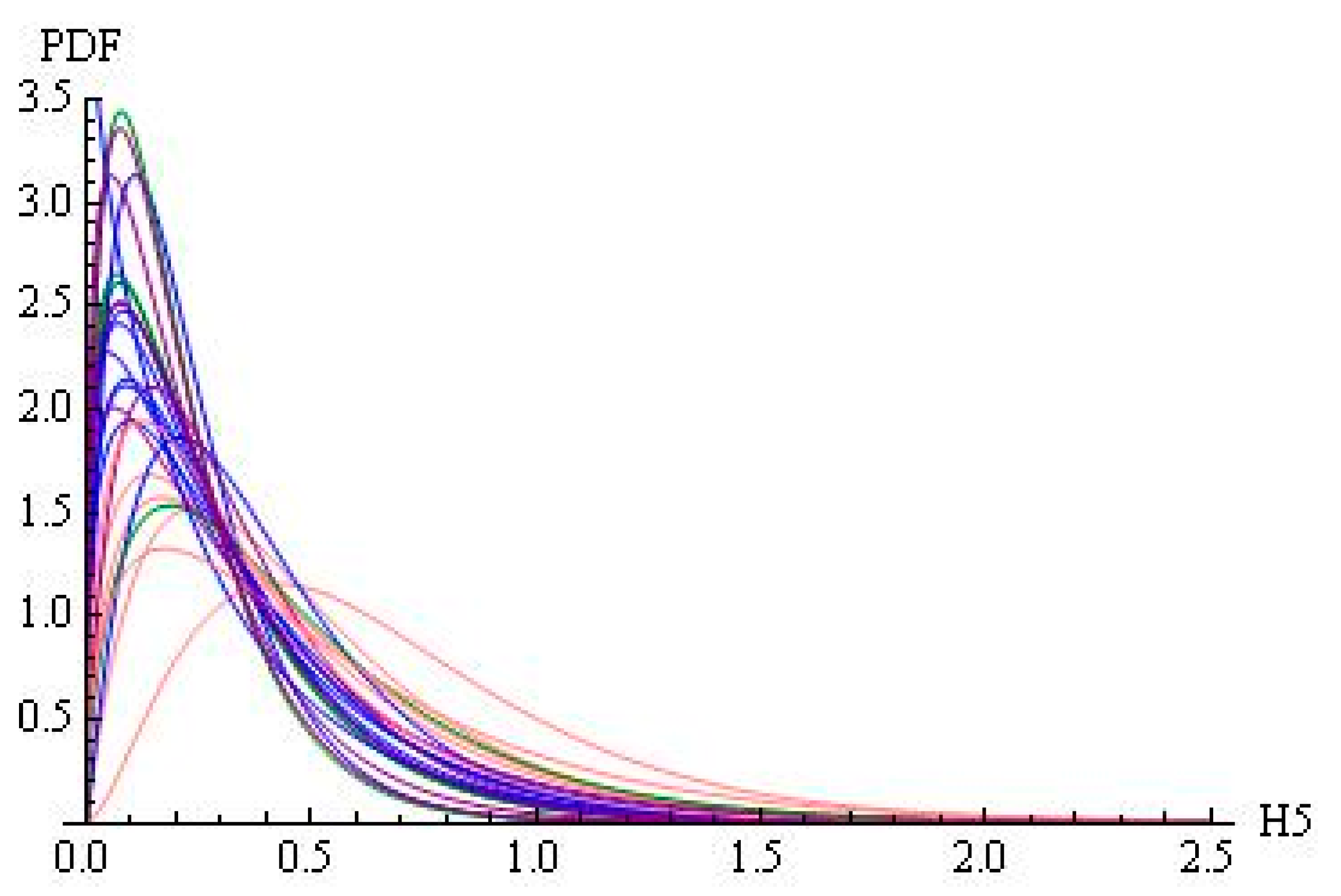
Figure 3.
Histograms of H5 for subjects Sk. Pink = Health, Green = Life, Blue = Physical, Purple = Social.
Figure 3.
Histograms of H5 for subjects Sk. Pink = Health, Green = Life, Blue = Physical, Purple = Social.

Figure 4.
Gamma Probability Density Functions of H5 for subjects Sk. Pink = Health, Green = Life, Blue = Physical, Purple = Social.
Figure 4.
Gamma Probability Density Functions of H5 for subjects Sk. Pink = Health, Green = Life, Blue = Physical, Purple = Social.
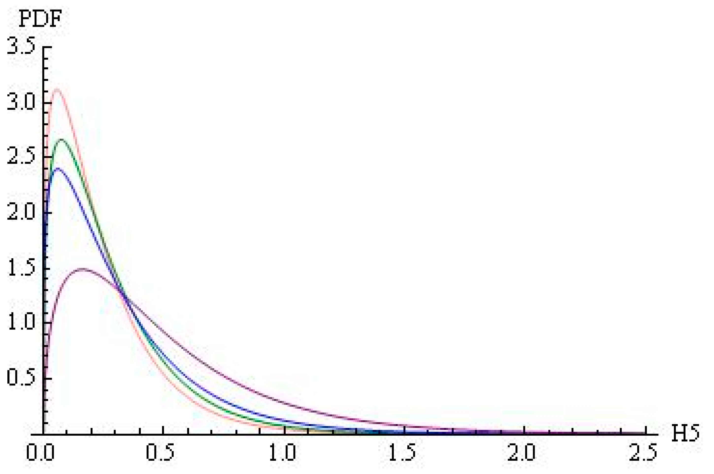
Table 1.
Description of acronyms and variables.
| Acronyms | Description |
|---|---|
| Ifa | Inefficiency a |
| Ifb | Inefficiency b |
| Iqa | Inequity a |
| Iqb | Inequity b |
| Variables | |
| Npub | Number of publications |
| Nart | Number of articles |
| Ngro | Number of citations including co-author’s citations |
| Nnet | Number of citations excluding co-author’s citations |
| Naut | Mean number of co-authors |
| H1 | H-index based on publications |
| H2 | H-index based on articles |
| H3 | H-index based on net citations per article |
| H4 | Net per-capita H-index based on articles |
| H5 | Net per-capita per-year H-index based on articles |
| ∆Hh = Hh − Hh+1 | H-index improvement, h = 1, 2, 3, 4, 5 |
| Dj | Dummy variable for discipline j (j = 1,…, 27) (i.e., Dj takes value 1 for a discipline j and 0 for disciplines other than j) |
| Sk | Dummy variable for subject k (k = 1, 2, 3, 4) (i.e., Sk takes value 1 for a subject k and 0 for subjects other than k) |
| Aaut | Dummy variable for age (Aaut = 1 if author’s first publication is after 2009, otherwise Aaut = 0) |
Table 2.
Summary statistics on independent variables for subjects Sk. Notations: mean (SD) is in the first row for each subject, median [min–max] is in the second row for each subject; in columns, Npub = No. publications, Nart = No. articles, Naut = No. co-authors, Ngro = No. gross citations, Nnet = No. net citations.
| Npub | Nart | Naut | Ngro | Nnet | |
|---|---|---|---|---|---|
| Health | 5.112 (14.302) | 5.057 (14.032) | 12.875 (74.372) | 8.091 (24.841) | 7.966 (24.302) |
| 1 [1–444] | 1 [1–435] | 6.400 [1–2060] | 2.333 [0–988] | 2.333 [0–965] | |
| Life | 5.203 (11.979) | 5.171 (11.901) | 7.904 (15.337) | 9.480 (21.171) | 9.289 (20.764) |
| 2 [1–206] | 2 [1–206] | 6 [1–461] | 3 [0–358] | 3 [0–358] | |
| Physical | 5.709 (17.865) | 5.687 (17.835) | 15.874 (135.262) | 5.646 (13.910) | 5.510 (13.720) |
| 2 [1–468] | 2 [1–468] | 4.500 [1–2837.009] | 1.667 [0–256] | 1.600 [0–256] | |
| Social | 2.909 (4.246) | 2.906 (4.237) | 3.061 (9.622) | 4.775 (14.610) | 4.737 (14.590) |
| 1 [1–39] | 1 [1–39] | 2 [1–228] | 1 [0–212] | 1 [0–212] |
Table 3.
Summary statistics on all H-indexes for subjects Sk. Notations: mean (SD) is in the first row for each subject, median [min–max] is in the second row for each subject.
Table 3.
Summary statistics on all H-indexes for subjects Sk. Notations: mean (SD) is in the first row for each subject, median [min–max] is in the second row for each subject.
| H1 | H2 | H3 | H4 | H5 | |
|---|---|---|---|---|---|
| Health | 1.916 (3.151) | 1.916 (3.151) | 1.889 (3.033) | 0.329 (0.559) | 0.173 (0.249) |
| 1 [0–43] | 1 [0–43] | 1 [0–39] | 0.167 [0–8.367] | 0.111 [0–4.111] | |
| Life | 2.188 (3.525) | 2.188 (3.525) | 2.147 (3.300) | 0.423 (0.681) | 0.216 (0.291) |
| 1 [0–72] | 1 [0–72] | 1 [0–60] | 0.200 [0–6.479] | 0.143 [0–3.167] | |
| Physical | 1.774 (2.913) | 1.774 (2.913) | 1.728 (2.747) | 0.430 (0.705) | 0.220 (0.320) |
| 1 [0–42] | 1 [0–42] | 1 [0–37] | 0.225 [0–12.417] | 0.125 [0–5.333] | |
| Social | 1.209 (1.606) | 1.209 (1.606) | 1.198 (1.576) | 0.601 (0.839) | 0.313 (0.419) |
| 1 [0–12] | 1 [0–12] | 1 [0–12] | 0.333 [0–6] | 0.167 [0–2.667] |
Table 4.
ANOVA on Npub—Nart for disciplines. DF = degree of freedom, ** = significant at 99%. Npub = No. publications, Nart = No. articles.
Table 4.
ANOVA on Npub—Nart for disciplines. DF = degree of freedom, ** = significant at 99%. Npub = No. publications, Nart = No. articles.
| DF | Sum Squares | % Tot | Mean Squares | F Value | p-Value | Significance | |
|---|---|---|---|---|---|---|---|
| ∆H1 = H1 − H2 | |||||||
| Disciplines | 24 | 4.67 | 0.47 | 0.194473 | 1.9541 | 0.003504 | ** |
| Residuals | 9972 | 992.43 | 99.53 | 0.099521 |
Table 5.
ANOVA on Npub—Nart for subjects. DF = degree of freedom, *** = significant at 99.9%. Npub = No. publications, Nart = No. articles.
Table 5.
ANOVA on Npub—Nart for subjects. DF = degree of freedom, *** = significant at 99.9%. Npub = No. publications, Nart = No. articles.
| DF | Sum Squares | % Tot | Mean Squares | F Value | p-Value | Significance | |
|---|---|---|---|---|---|---|---|
| ∆H1 = H1 − H2 | |||||||
| Subjects | 3 | 2.86 | 0.29 | 0.95231 | 9.5716 | 2.621 × 10−06 | *** |
| Residuals | 9993 | 994.24 | 99.71 | 0.09949 |
Table 6.
Npub and Nart in subjects Sk. Nobs = No. observations, Npub = No. publications, Nart = No. articles.
Table 6.
Npub and Nart in subjects Sk. Nobs = No. observations, Npub = No. publications, Nart = No. articles.
| Nobs | Npub | Nart | ∆ | % | |
|---|---|---|---|---|---|
| Health | 3698 | 18,904 | 18,702 | 202 | 1.07 |
| Life | 1834 | 9543 | 9483 | 60 | 0.63 |
| Physical | 3733 | 21,311 | 21,230 | 81 | 0.38 |
| Social | 733 | 2132 | 2130 | 2 | 0.09 |
Table 7.
ANOVA on Ngro—Nnet for disciplines. DF = degree of freedom, *** and * = significant at 99.9% and 95%. Ngro = No. gross citations, Nnet = No. net citations.
Table 7.
ANOVA on Ngro—Nnet for disciplines. DF = degree of freedom, *** and * = significant at 99.9% and 95%. Ngro = No. gross citations, Nnet = No. net citations.
| DF | Sum Squares | % Tot | Mean Squares | F Value | p-Value | Significance | |
|---|---|---|---|---|---|---|---|
| ∆H2 = H2 − H3 | 1 | 3140.6 | 26.79 | 3140.63 | 3663.7511 | <2 × 10⁻¹⁶ | *** |
| Disciplines | 24 | 34.0 | 0.29 | 1.42 | 1.6547 | 0.02316 | * |
| Residuals | 9971 | 8547.3 | 72.92 | 0.86 |
Table 8.
ANOVA on Ngro—Nnet for subjects. DF = degree of freedom, *** and * = significant at 99.9% and 95%. Ngro = No. gross citations, Nnet = No. net citations.
Table 8.
ANOVA on Ngro—Nnet for subjects. DF = degree of freedom, *** and * = significant at 99.9% and 95%. Ngro = No. gross citations, Nnet = No. net citations.
| DF | Sum Squares | % Tot | Mean Squares | F Value | p-Value | Significance | |
|---|---|---|---|---|---|---|---|
| ∆H2 = H2 − H3 | 1 | 3140.6 | 26.79 | 3140.63 | 3659.968 | <2 × 10⁻¹⁶ | *** |
| Subjects | 3 | 7.2 | 0.06 | 2.40 | 2.792 | 0.0389 | * |
| Residuals | 9992 | 8574.2 | 73.15 | 0.86 |
Table 9.
Linear regression of Ngro—Nnet on ∆H2 and subjects Sk. *** and ** = significant at 99.9% and 99%. Ngro = No. gross citations, Nnet = No. net citations.
Table 9.
Linear regression of Ngro—Nnet on ∆H2 and subjects Sk. *** and ** = significant at 99.9% and 99%. Ngro = No. gross citations, Nnet = No. net citations.
| Estimate | Std. Error | t Value | p-Value | Significance | |
|---|---|---|---|---|---|
| ∆H2 = H2 − H3 | 2.00998 | 0.03325 | 60.442 | <2 × 10⁻¹⁶ | *** |
| Health | 0.07116 | 0.01526 | 4.663 | 3.16 × 10−06 | *** |
| Life | 0.10768 | 0.02167 | 4.968 | 6.88 × 10−07 | *** |
| Physical | 0.04189 | 0.01524 | 2.748 | 0.006 | ** |
| Social | 0.01604 | 0.03422 | 0.469 | 0.639 |
Table 10.
ANOVA on Nnet for disciplines. DF = degree of freedom, *** = significant at 99.9%. Nnet = No. net citations, Naut = No. co-authors.
Table 10.
ANOVA on Nnet for disciplines. DF = degree of freedom, *** = significant at 99.9%. Nnet = No. net citations, Naut = No. co-authors.
| DF | Sum Squares | % Tot | Mean Squares | F Value | p-Value | Significance | |
|---|---|---|---|---|---|---|---|
| Naut | 1 | 25,395 | 0.66 | 25,395 | 70.0203 | <2.2 × 10⁻¹⁶ | *** |
| ∆H3 = H3 − H4 | 1 | 168,777 | 4.38 | 168,777 | 465.3608 | <2.2 × 10⁻¹⁶ | *** |
| Disciplines | 24 | 46,907 | 1.22 | 1954 | 5.3889 | 2.728 × 10⁻¹⁶ | *** |
| Residuals | 9970 | 3,615,927 | 93.75 | 363 |
Table 11.
ANOVA on Nnet for subjects. DF = degree of freedom, *** = significant at 99.9%. Nnet = No. net citations, Naut = No. co-authors.
Table 11.
ANOVA on Nnet for subjects. DF = degree of freedom, *** = significant at 99.9%. Nnet = No. net citations, Naut = No. co-authors.
| DF | Sum Squares | % Tot | Mean Squares | F Value | p-Value | Significance | |
|---|---|---|---|---|---|---|---|
| Naut | 1 | 25,395 | 0.66 | 25,395 | 69.551 | <2.2 × 10⁻¹⁶ | *** |
| ∆H3 = H3 − H4 | 1 | 168,777 | 4.38 | 168,777 | 462.241 | <2.2 × 10⁻¹⁶ | *** |
| Subjects | 3 | 14,837 | 0.38 | 4946 | 13.545 | 8.129 × 10−09 | *** |
| Residuals | 9991 | 3,647,997 | 94.58 | 365 |
Table 12.
Linear regression of Nnet on Naut, ∆H3 and subjects Sk. *** = significant at 99.9%. Nnet = No. net citations, Naut = No. co-authors.
Table 12.
Linear regression of Nnet on Naut, ∆H3 and subjects Sk. *** = significant at 99.9%. Nnet = No. net citations, Naut = No. co-authors.
| Estimate | Std. Error | t Value | p-Value | Significance | |
|---|---|---|---|---|---|
| Naut | 0.009705 | 0.002054 | 4.725 | 2.33 × 10−06 | *** |
| ∆H3 = H3 − H4 | 1.680821 | 0.080859 | 20.787 | <2 × 10⁻¹⁶ | *** |
| Health | 5.220720 | 0.337960 | 15.448 | <2 × 10⁻¹⁶ | *** |
| Life | 6.315327 | 0.466899 | 13.526 | <2 × 10⁻¹⁶ | *** |
| Physical | 3.174912 | 0.329690 | 9.630 | <2 × 10⁻¹⁶ | *** |
| Social | 3.703891 | 0.707383 | 5.236 | 1.67 × 10−07 | *** |
Table 13.
Differences between subjects Sk (below diagonal) and related p-values (above diagonal).
| Health | Life | Physical | Social | |
|---|---|---|---|---|
| Health | - | 0.0450 | 4.1 × 10−06 | 0.0508 |
| Life | 1.0946 | - | 9.3 × 10−09 | 0.0019 |
| Physical | −2.0458 | −3.1404 | - | 0.4944 |
| Social | −1.5168 | −2.6114 | −0.529 | - |
Table 14.
ANOVA on Nnet for disciplines. DF = degree of freedom, *** = significant at 99.9%. Nnet = No. net citations, Naut = No. co-authors, Aaut = 1 for inexpert authors.
Table 14.
ANOVA on Nnet for disciplines. DF = degree of freedom, *** = significant at 99.9%. Nnet = No. net citations, Naut = No. co-authors, Aaut = 1 for inexpert authors.
| DF | Sum Squares | % Tot | Mean Squares | F Value | p-Value | Significance | |
|---|---|---|---|---|---|---|---|
| Naut | 1 | 25,395 | 0.66 | 25,395 | 70.9415 | <2.2 × 10⁻¹⁶ | *** |
| Aaut | 1 | 172,892 | 4.48 | 172,892 | 482.9768 | <2.2 × 10⁻¹⁶ | *** |
| ∆H4 = H4 − H5 | 1 | 17,869 | 0.46 | 17,869 | 49.9175 | 1.711 × 10⁻¹² | *** |
| Disciplines | 24 | 72,237 | 1.87 | 3010 | 8.4082 | <2.2 × 10⁻¹⁶ | *** |
| Residuals | 9969 | 3,568,613 | 92.52 | 358 |
Table 15.
ANOVA on Nnet for subjects. DF = degree of freedom, *** = significant at 99.9%. Nnet = No. net citations, Naut = No. co-authors, Aaut = 1 for inexpert authors.
Table 15.
ANOVA on Nnet for subjects. DF = degree of freedom, *** = significant at 99.9%. Nnet = No. net citations, Naut = No. co-authors, Aaut = 1 for inexpert authors.
| DF | Sum Squares | % Tot | Mean Squares | F Value | p-Value | Significance | |
|---|---|---|---|---|---|---|---|
| Naut | 1 | 25,395 | 0.66 | 25,395 | 70.158 | <2.2 × 10⁻¹⁶ | *** |
| Aaut | 1 | 172,892 | 4.48 | 172,892 | 477.644 | <2.2 × 10⁻¹⁶ | *** |
| ∆H4 = H4 − H5 | 1 | 17,869 | 0.46 | 17,869 | 49.366 | 2.262 × 10⁻¹² | *** |
| Subjects | 3 | 24,794 | 0.64 | 8265 | 22.833 | 1.002 × 10⁻¹⁴ | *** |
| Residuals | 9990 | 3,616,056 | 93.75 | 362 |
Table 16.
Linear regression of Nnet on Naut, Aaut, ∆H4 and subjects Sk. *** = significant at 99.9%. Nnet = No. net citations, Naut = No. co-authors, Aaut = 1 for inexpert authors.
Table 16.
Linear regression of Nnet on Naut, Aaut, ∆H4 and subjects Sk. *** = significant at 99.9%. Nnet = No. net citations, Naut = No. co-authors, Aaut = 1 for inexpert authors.
| Estimate | Std. Error | t Value | p-Value | Significance | |
|---|---|---|---|---|---|
| Naut | 0.017634 | 0.002015 | 8.752 | <2 × 10⁻¹⁶ | *** |
| Aaut | −8.844221 | 0.408641 | −21.643 | <2 × 10⁻¹⁶ | *** |
| ∆H4 = H4 − H5 | −0.458533 | 0.498655 | −0.920 | 0.358 | |
| Health | 12.266976 | 0.398495 | 30.783 | <2 × 10⁻¹⁶ | *** |
| Life | 13.541654 | 0.512477 | 26.424 | <2 × 10⁻¹⁶ | *** |
| Physical | 9.790119 | 0.409115 | 23.930 | <2 × 10⁻¹⁶ | *** |
| Social | 9.049664 | 0.757110 | 11.953 | <2 × 10⁻¹⁶ | *** |
Table 17.
Differences between subjects Sk (below diagonal) and related p-values (above diagonal).
| Health | Life | Physical | Social | |
|---|---|---|---|---|
| Health | - | 0.0191 | 2.2 × 10−08 | 3.1 × 10−05 |
| Life | 1.2747 | - | 5.1 × 10⁻¹² | 6.9 × 10−08 |
| Physical | −2.4769 | −3.7515 | - | 0.336 |
| Social | −3.2173 | −4.4920 | −0.7405 | - |
Table 18.
ANOVA on Ngro for disciplines. DF = degree of freedom, *** = significant at 99.9%. Ngro = No. gross citations, Nnet = No. net citations, Naut = No. co-authors, Aaut = 1 for inexpert authors.
Table 18.
ANOVA on Ngro for disciplines. DF = degree of freedom, *** = significant at 99.9%. Ngro = No. gross citations, Nnet = No. net citations, Naut = No. co-authors, Aaut = 1 for inexpert authors.
| DF | Sum Squares | % Tot | Mean Squares | F Value | p-Value | Significance | |
|---|---|---|---|---|---|---|---|
| Nnet | 1 | 3,790,911 | 99.72 | 3,790,911 | 3.1661 × 10+06 | <2.2 × 10⁻¹⁶ | *** |
| Naut | 1 | 302 | 0.01 | 302 | 2.5244 × 10+02 | <2.2 × 10⁻¹⁶ | *** |
| Aaut | 1 | 19 | 0.00 | 19 | 1.5815 × 10+01 | 7.053 × 10−05 | *** |
| ∆H5 = H1 − H5 | 1 | 1562 | 0.04 | 1562 | 1.3042 × 10+03 | <2.2 × 10⁻¹⁶ | *** |
| Disciplines | 24 | 71 | 0.00 | 3 | 2.4638 × 10+00 | 8.895 × 10−05 | *** |
| Residuals | 7123 | 8529 | 0.22 | 1 |
Table 19.
ANOVA on Ngro for subjects. DF = degree of freedom, *** and * = significant at 99.9% and 95%. Ngro = No. gross citations, Nnet = No. net citations, Naut = No. co-authors, Aaut = 1 for inexpert authors.
Table 19.
ANOVA on Ngro for subjects. DF = degree of freedom, *** and * = significant at 99.9% and 95%. Ngro = No. gross citations, Nnet = No. net citations, Naut = No. co-authors, Aaut = 1 for inexpert authors.
| DF | Sum Squares | % Tot | Mean Squares | F Value | p-Value | Significance | |
|---|---|---|---|---|---|---|---|
| Nnet | 1 | 3,790,911 | 99.72 | 3,790,911 | 3.1542 × 10+06 | <2.2 × 10⁻¹⁶ | *** |
| Naut | 1 | 302 | 0.01 | 302 | 2.5149 × 10+02 | <2.2 × 10⁻¹⁶ | *** |
| Aaut | 1 | 19 | 0.00 | 19 | 1.5756 × 10+01 | 7.277 × 10−05 | *** |
| ∆H5 = H1 − H5 | 1 | 1562 | 0.04 | 1562 | 1.2993 × 10+03 | <2.2 × 10⁻¹⁶ | *** |
| Subjects | 3 | 14 | 0.00 | 5 | 3.7473 × 10+00 | 0.01053 | * |
| Residuals | 7144 | 8586 | 0.23 | 1 |
Table 20.
Linear regression of Ngro on Nnet, Naut, Aaut, ∆H5, and subjects Sk. *** = significant at 99.9%. Ngro = No. gross citations, Nnet = No. net citations, Naut = No. co-authors, Aaut = 1 for inexpert authors.
Table 20.
Linear regression of Ngro on Nnet, Naut, Aaut, ∆H5, and subjects Sk. *** = significant at 99.9%. Ngro = No. gross citations, Nnet = No. net citations, Naut = No. co-authors, Aaut = 1 for inexpert authors.
| Estimate | Std. Error | t Value | p-Value | Significance | |
|---|---|---|---|---|---|
| Nnet | 1.0153304 | 0.0005870 | 1729.830 | <2 × 10⁻¹⁶ | *** |
| Naut | 0.0011305 | 0.0001229 | 9.200 | <2 × 10⁻¹⁶ | *** |
| Aaut | 0.1808438 | 0.0282857 | 6.393 | 1.72 × 10⁻¹⁰ | *** |
| ∆H5 = H1 − H5 | 0.1589654 | 0.0044038 | 36.097 | <2 × 10⁻¹⁶ | *** |
| Health | −0.4654963 | 0.0282006 | −16.507 | <2 × 10⁻¹⁶ | *** |
| Life | −0.4164853 | 0.0346145 | −12.032 | <2 × 10⁻¹⁶ | *** |
| Physical | −0.3747120 | 0.0275985 | −13.577 | <2 × 10⁻¹⁶ | *** |
| Social | −0.3403357 | 0.0523529 | −6.501 | 8.53 × 10⁻¹¹ | *** |
Table 21.
Percentages of authors characterised by H5 larger than 1, 1.5, 2, 2.5 and 3 for subjects Sk.
Table 21.
Percentages of authors characterised by H5 larger than 1, 1.5, 2, 2.5 and 3 for subjects Sk.
| H5 ≥ 1 | H5 ≥ 1.5 | H5 ≥ 2 | H5 ≥ 2.5 | H5 ≥ 3 | |
|---|---|---|---|---|---|
| Health | 0.01012250 | 0.00105278 | 0.00009720 | 0.00000083 | 0.00000006 |
| Life | 0.01899160 | 0.00260541 | 0.00031683 | 0.00003588 | 0.00000038 |
| Physical | 0.04220660 | 0.00922697 | 0.00182136 | 0.00033814 | 0.00006023 |
| Social | 0.14236600 | 0.04902840 | 0.01510380 | 0.00434077 | 0.00118783 |
Disclaimer/Publisher’s Note: The statements, opinions and data contained in all publications are solely those of the individual author(s) and contributor(s) and not of MDPI and/or the editor(s). MDPI and/or the editor(s) disclaim responsibility for any injury to people or property resulting from any ideas, methods, instructions or products referred to in the content. |
© 2024 by the authors. Licensee MDPI, Basel, Switzerland. This article is an open access article distributed under the terms and conditions of the Creative Commons Attribution (CC BY) license (https://creativecommons.org/licenses/by/4.0/).
Share and Cite
MDPI and ACS Style
Zagonari, F.; Foschi, P. Coping with the Inequity and Inefficiency of the H-Index: A Cross-Disciplinary Empirical Analysis. Publications 2024, 12, 12. https://doi.org/10.3390/publications12020012
AMA Style
Zagonari F, Foschi P. Coping with the Inequity and Inefficiency of the H-Index: A Cross-Disciplinary Empirical Analysis. Publications. 2024; 12(2):12. https://doi.org/10.3390/publications12020012
Chicago/Turabian StyleZagonari, Fabio, and Paolo Foschi. 2024. "Coping with the Inequity and Inefficiency of the H-Index: A Cross-Disciplinary Empirical Analysis" Publications 12, no. 2: 12. https://doi.org/10.3390/publications12020012
Note that from the first issue of 2016, this journal uses article numbers instead of page numbers. See further details here.