Heat Integration of a Boiler and Its Corresponding Environmental Study in an Oleochemical Production Plant: An Industry Case Study in Malaysia

Abstract

The growing demands for oleochemical products are expected to reach approximately RM 157.59 billion by 2026 due to an increased drive from the food and beverages, chemicals, and pharmaceutical industries. However, this will lead to an increase in energy consumption and subsequent flue gas emission. Proper utilization of waste gas recovery systems is thus a major research area, focusing on reducing fuel consumption and emissions of greenhouse gases without affecting process performance. In this paper, a palm oil-based oleochemical plant is studied. The fuel consumption and emission of flue gas from a thermal oil boiler were measured and the feasibility of implementation of a waste heat recovery system and its environmental impact study. The results show that the implementation of such a system can reduce natural fuel gas consumption by 17.29% and approximately 149.29 t per annum of carbon dioxide gas (CO₂). Moreover, the concentration of CO₂ released into highly-populated communities is estimated through a Gaussian Plume Model at different wind speed conditions. The preliminary results show that the CO₂ concentration at two locations—an apartment and a local school located within 1.5 km of the plant—is well below the concentration limit of 1.938 g/m³ recommended by the Wisconsin Department of Health and Services.

1. Introduction

Oleochemical products can be derived from animal fats or vegetable oils. Since vegetable oils account for nearly 80% of the total fat and oil production, it is also the main source for oleochemical production, especially from palm, coconut, soybean, and sunflower [1,2]. The oil extracted from the flesh of the oil palm fruit (species Elaeis Guineensis Jacq.), in its native setting, is generally a vibrant orange colour. Originating in South Africa, this fine vegetation was introduced to Malaysia in the early 1870s by the British and was planted commercially in 1917 [3]. Being the world’s second-largest palm oil exporter (after its neighbouring country, Indonesia), Malaysia accounts for 39% and 44% of the global production and exportation, respectively. Most of the oleochemical products in Malaysia are largely derived from palm oil [4,5]. With the global oleochemical market showed increase in demand since 2014 owing to increasing petrochemical prices and rising environmental concerns [6], the energy demand for the production process in Malaysia is expected to follow suit [7,8]—chemical manufacturing accounted for 12% of the country’s total energy consumption in 2016. Malaysia is, therefore, expected to experience an increasing demand for energy consumption and a subsequent rise in carbon dioxide gas emission [9]. Faced with global warming and increasing fuel prices, manufacturing industries are constantly looking for ways to reduce greenhouse gases and fuel consumption caused by their processes. Proper utilization of waste gas recovery systems has, therefore, become a major research area for this industry, focusing on reducing environmental impacts without affecting process performance.

Heat integration (HI) is an industrial technique used to minimize energy consumption and maximize thermal energy recovery. Albeit the technique was first introduced by Linnhoff and Flower to maximize utility cost-saving through waste heat recovery in the 1970s, systematic methods to optimize heat recovery, cost-saving and greenhouse gas emissions are still studied today [10,11]. The development of the HI technique over the past 40 years through pinch analysis and mathematical programming was reviewed by Klemeš et al. in 2012 [12]. They concluded that recent overviews of HI focus on the sustainability of the technique in current operating processes [12]. HI is currently streamlined into two approaches: HI within individual process (waste heat recovery system), also referred to as intra-plant HI; and total site HI system, which is also known as inter-plant HI.

Largely practiced at plants, total site heat integration (TSHI) incorporates a multitude of processes that are linked to a central utility system, tying together services and production deliverables [13]. Amir H. Tarighaleslami et. al. studied different approaches to TSHI and compared two methods—conventional total site targeting (CTST) and unified total site targeting (UTST). The latter utilizes total process-level utility targets as the basis for total site utility targets, whereas CTST is similar to pinch analysis, where excess heat is produced (surplus) or absorbed (deficit) by the process.

Table 1. Comparison between UTST and CTST methods [14].

TSHI APPROACHES	UTST	CTST
Matching of Utility Heat Exchanger	Series	Series and Parallel
Drawback of System	Slightly lower heat recovery targets	Dependency on separate processes, resulting in complications with regards to operation and control.

shows a comparison of both techniques: It was found that the recovery targets in the UTST method are slightly lower compared to CTST; however, they have more realistic expectations [14]. Although TSHI reduces energy consumption and resolves waste heat-caused conflicts, the operability of such a system should be further discussed, as the costs and energy produced are highly dependent on retrofitting functions (operability and implementation of a heat exchanger network). Sofie Marton et. al. dissected the operability of heat integration into four subsequent categories: flexibility, controllability, start-up and shutdown procedures, and reliability of the system. Such implementations have required certain changes in operations, resulting in additional constraints in system design [15]. Therefore, such systems require decisive planning and careful consideration upon implementation. Peng et. al. have extensively studied comprehensive planning and framework design for TSHI. Owing to their efforts, the factors that have a direct impact on the feasibility of integrating industrial clusters with renewable energy have been identified and discussed; they include economic feasibility and system reliability. The economy is a major defining factor for project feasibility; heavily influenced by the price of fossil fuel, it has a direct impact on payback time in investments. The advancement of new technology is expected to reduce the cost of implementation of this current broadly-accepted technology. Subsequently, the period of implementation is of paramount importance in defining the feasibility of a project from an economic perspective. In addition, the life cycle of key operating units such as boilers and heat exchangers should be further studied to minimise the impacts of equipment breakdown on production, simultaneously maximising the reliability of the TSHI system [16].

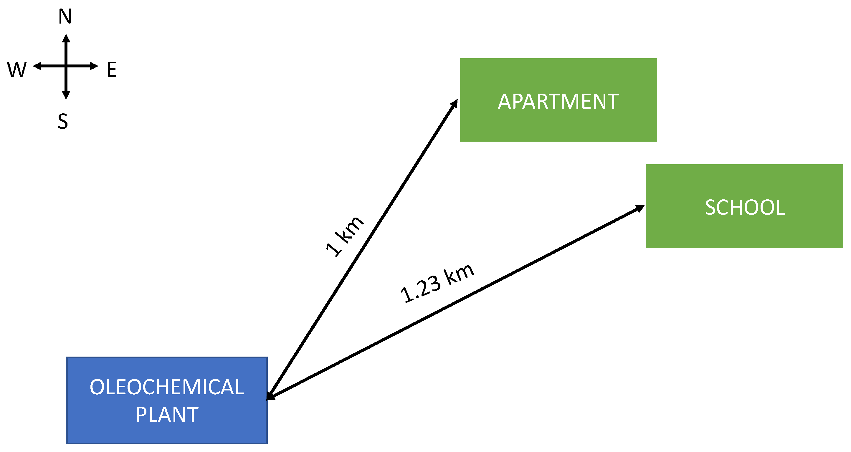
Meanwhile, with the rapid growth of industrial development, it is essential to keep air quality in check to avoid adverse impacts on human health and biodiversity. Therefore, the Department of Environment (DOE) Malaysia has been entrusted with the task of monitoring air quality nationwide and controlling new industry development projects through the Environmental Impact Assessment Order (1987). Under this order, DOE requires the Environmental Impact Assessment (EIA) reports of prescribed industrial activities to be submitted for approval before a project is implemented. The reports will be assessed based on the Environmental Quality (Clean Air) Regulation 1978 enforced by DOE in limiting and controlling the air pollutant emissions. The regulation lists factors of air pollution including the location of industrial facilities adjacent to residential areas, waste burning, and emission of dark smoke and air pollutants, which serve as a guideline for DOE and industries in order to protect air quality and reduce air pollution.

Currently, most oleochemical plants in Malaysia use boilers as a heat source. The technical standards for boilers used in heat and power generation as set by the Federal Government Gazette Malaysia are shown in

Table A1. Limit values and technical standards for boiler [34].

FUEL TYPE	POLLUTANT	CAPACITY	LIMIT VALUE	MONITORING
Solid and Liquid Fuels	Sum of SO2 and SO3, expressed of SO2	>10 MWe	500 mg/m3	Continuous *
	Sum of NO2 and NO3, expressed of NO2	>10 MWe	500 mg/m3	Continuous *
	Hydrogen Chloride (HCl)	10< C <100 MWe	200 mg/m3	Periodic
	Hydrogen Chloride (HCl)	≥100 MWe	100 mg/m3	Periodic
	Hydrogen Fluoride (HF)	10< C <100 MWe	30 mg/m3	Periodic
	Hydrogen Fluoride (HF)	≥100 MWe	15 mg/m3	Periodic
	Carbon Monoxide (CO)	>10 MWe	200 mg/m3	Continuous *
	Total PM	>10 MWe	50 mg/m3	Continuous *
	Mercury (Hg)	>10 MWe	0.03 mg/m3	Periodic
	PCDD/PCDF	>10 MWe	0.1 ng TEQ/m3	Periodic
Gaseous Fuels	Sum of NO2 and NO3, expressed of NO2	>10 MWe	350 mg/m3	Continuous *
	Carbon Monoxide (CO)	>10 MWe	50 mg/m3	Continuous *
	Total PM	>10 MWe	5 mg/m3	Periodic

* Averaging time for continuous monitoring is 30 min.

, whereas the standards set for stack gas emissions under the Environmental Quality (Clean Air) Regulation 1978 are as listed in

Table A2. Stack gas emission standards [35].

POLLUTION	EMISSION SOURCES	STANDARDS
1. Dark Smoke	1.1. Solid Fuel Equipment to Facilities	Ringlemann Chart No.2
	1.2. Equipment Using Other Types of Fuel	Ringlemann Chart No.1
2. Dust	2.1. Facilities Used for the Heating of Metal Other Thank Cold Blast Foundry Cupola	0.2 gm/Nm3
	2.2. Facilities Discharging Dust Containing Asbestos and Free Silica	0.12 gm/Nm3
	2.3. Portland Cement Manufacturing:
	2.3.1. Kiln	0.2 gm/Nm3
	2.3.2. Clinker, Cooler, Grinder, Others	0.1 gm/Nm3
	2.4. Asphalt Concrete/Bituminous Mixing Plant:
	2.4.1. Stationary Plant	0.3 gm/Nm3
	2.4.2. Mobile Plant	0.4 gm/Nm3
	2.5. Other Sources	0.4 gm/Nm3
3. Metal and Metallic Compound
3.1. Mercury	Industry	0.01 gm/Nm3
3.2. Cadmium	Industry	0.015 gm/Nm3
3.3. Lead	Industry	0.025 gm/Nm3
3.4. Antimony	Industry	0.025 gm/Nm3
3.5. Arsenic	Industry	0.025 gm/Nm3
3.6. Zinc	Industry	0.1 gm/Nm3
3.7. Copper	Industry	0.1 gm/Nm3
4. Gases
4.1. Acid Gases	Sulphuric Acid Manufacturing	3.5 gm of SO3/Nm3 and No Persistent Mist
4.2. Sulphuric Acid Mist or SO3	Any Sources Other Than 4.1.	0.2 gm of SO3/Nm3 and No Persistent Mist
4.3. Chlorine Gas	Any Source	0.2 gm of HCl/Nm3
4.4. HCl	Any Source	0.2 gm of HCl/Nm3
4.5. Fluorine, Hydrofluoric Acid, Inorganic Compound	Aluminium Manufacturing from Alumina	0.2 gm of Hydrofluoric Acid/Nm3
4.6. - do -	Any Sources Other Than 4.5.	0.1 gm of Hydrofluoric Acid/Nm3
4.7. Hydrogen Sulphide	Any Source	5 ppm (Vol%)
4.8. NOX	Acid Nitric Manufacturing	1.7 gm of SO3/Nm3 and Substantially Colourless
4.9. SOX	Any Sources Other Than 4.8.	2.0 gm SO3/Nm3

. One disadvantage of boiler use is continuous emission of flue gas during the combustion process. Hence, it is important to conduct an air quality assessment to minimise its impact on the environment. A few steps are required in an air quality assessment. Firstly, a site survey is conducted to assess the impact of nearby existing industrial activities on air quality. Therefore, a careful layout of monitoring points is required to effectively assess existing air pollution sources near the proposed development. The data required to evaluate the cumulative impact of air pollutant emissions such as air pollutant source inventory, stack emission data and ambient air quality can be obtained directly from the surrounding industrial concerns or through DOE. After the collection of data, modelling of air quality is carried out to assess the air pollutant concentration emitted during the industrial activity. There are several factors to be considered, such as stack height and emission rate, meteorological conditions, topographic consideration and population consideration. Based on the results, an impact assessment is conducted and mitigating measures are recommended to reduce the environmental impacts below a level of significance [17].

As shown in Figure 1, there are three air quality models: deterministic models, statistical models, and physical models. Deterministic models deal with different types of numerical approximations in the solution, representing relevant atmospheric dispersion physical processes and are highly favourable for long-term plans. On the other hand, statistical models utilise an established statistical relationship between meteorological and other limitations to calculate the ambient air concentration, and these are most favourable for the short-term forecast of concentrations. In physical models, a physical experiment is carried out on a smaller scale to mimic the important features of the original process. Although the variables are easily controlled, physical models tend to incur higher costs compared to the other two models [18]. This paper focuses on deterministic models. There are two types of deterministic models: steady state and time dependent. Unlike time-dependent models, steady state models are independent of time variables. Research performed by Lutman ER et. al. compared the prediction of particle dispersion between the Gaussian plume model and the Lagrangian particle dispersion model. Studies have shown that the differences in modelling results between these two models are insignificant. While the Lagrangian model yields more realistic results, the Gaussian model appears to be a more appropriate tool for environmental assessment as it is more user friendly, though the results tend to be marginally over-estimated [19].

Gaussian plume model is one of the most popular air pollution dispersion models and it is the basis for most of the air pollution modelling software distributed by the EPA [20]. Many researchers have developed advanced Gaussian plume models such as AERMOD, CTDM or ADMS to provide more accurate air quality forecasts [21,22,23,24,25]. Researchers in the University of Messina and University of Catania, Italy carried out a study on the implementation of theoretical Gaussian plume model on a small scale. The results reveal that the error of the Gaussian plume model is consistently below 7% in all configurations, showing a positive compliance amongst the measured and modelled data. Therefore, it can be concluded that the near real-time nature of the Gaussian plume model makes it a powerful tool to analyse and predict the dispersion of pollutants for regulatory purposes [26,27].

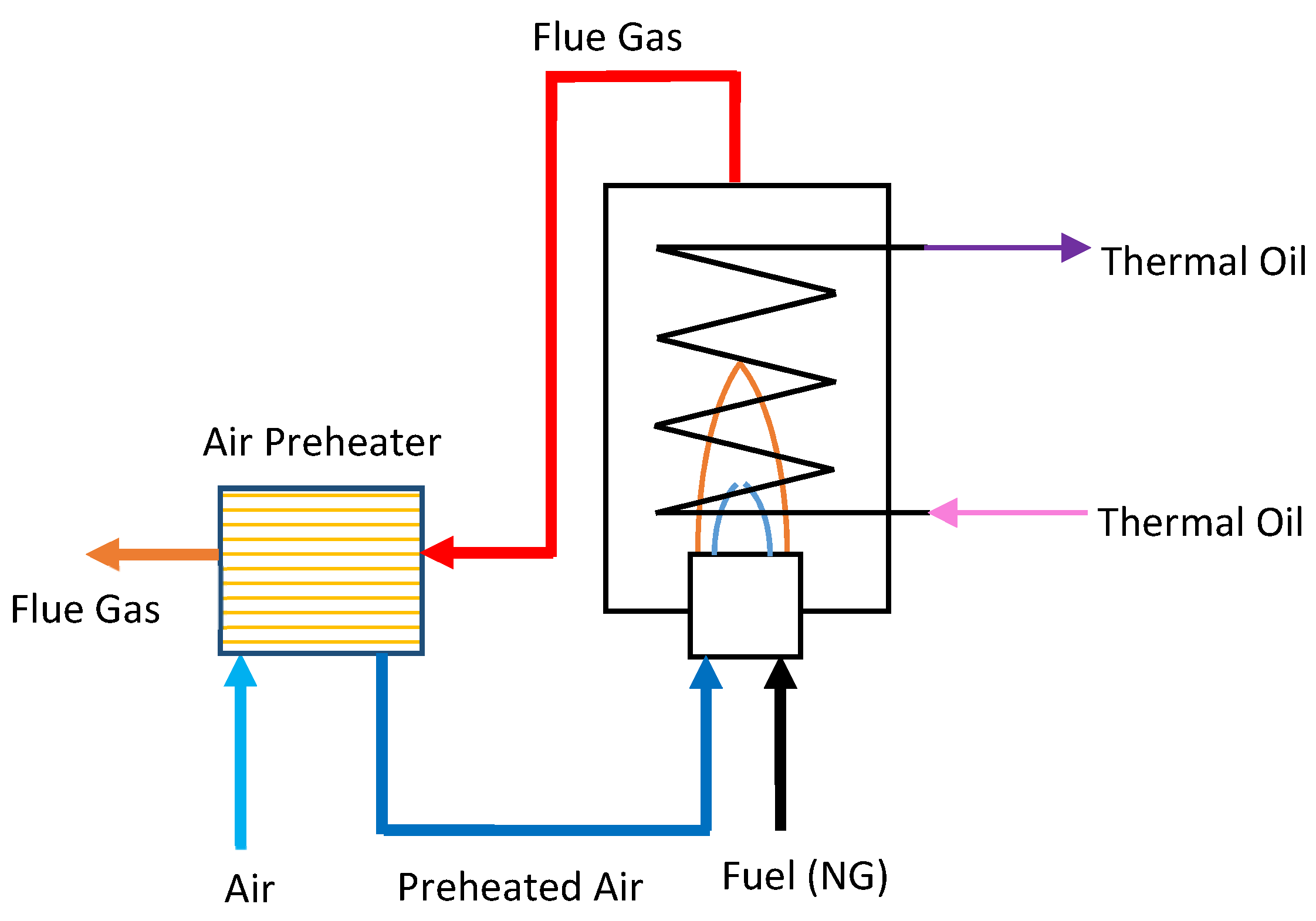
This study presents an innovative heat integration approach to a boiler in an oleochemical production plant, as shown in Figure 2b. To harvest waste heat released from the boiler exhaust, an air preheater is proposed to be installed on the thermal oil boiler to allow heat transfer between hot flue gas and fresh air. The main objective of the study is to perform a numerical study on the economic and environmental benefits of implementing waste heat recovery around a thermal oil boiler. The dew point of flue gas is also determined to prevent gas species condensation as it can result in stack wall corrosion [28]. Another desired outcome of this approach is a lower level of carbon dioxide emission to the surrounding neighbourhood.

2. Materials and Methods

The information used in this research is provided by the industry partner or obtained from HYSYS software, AspenTech Locations, Bedford, MA, USA. As this is a collaboration work with an industry partner, Microsoft Excel is used as the calculation tool.

2.1. Boiler System Heat Integration

Figure 3 shows the workflow diagram of the boiler system heat integration process, which begins with an input of the boiler data provided by the industry partner: mass flowrate, pressure (P), temperature (T), and the composition of air and natural gas fuel (NG). After inserting the given information and the preferred conditions for the flue gas outlet stream into an Excel spreadsheet, the premix temperature (T_premix) and the pressure of both air and NG is determined using enthalpy balance between the two feed streams. The flue gas temperature obtained from the operating data of the industry is then compared to the dew point (DP) of flue gas calculated using the auto goal-seek function in Visual Basic code as shown in Figure A1. As shown in Figure A2, a warning sign will pop out when the temperature of flue gas exceeds the theoretical DP of the flue gas. It is important to ensure that the flue gas temperature is well above the theoretical DP to prevent the formation of corrosion in the boiler stack as a result of flue gas condensation.

After heat has been exchanged at the economizer (Figure 2b), the revised temperature and pressure of air and flue gas (T* and P*) are determined. The energy and cost savings resulting from the newly conditioned flue gas are calculated through a comparison with the amount of natural gas fuel used before the system is implemented. After obtaining the data for cost saving, the payback time for the investment made in implementing the waste heat recovery system can also be calculated using Equations (1) and (2):

$$ROR=\frac{Costsavingperyear}{Originalinvestment}\times 100\%$$

(1)

ROR = Rate of return

$$PBT=\frac{100\%}{ROR}$$

(2)

PBT = Payback period

2.2. Gausian Plume Model

Gaussian plume model can be generated by inputting the data provided by the industry source, including the estimated flow rate of carbon dioxide gas released during the heat integration calculation, diameter of the flare stack, gas emission temperature, referential temperature, wind speed, distance between the specific location and the flare stack, and elevation temperature. Then, plume rise calculation under different scenarios, as shown in Figure A3, is carried out. After plume rise and effective stack height are determined, the concentration of carbon dioxide gas released is calculated using Equation (3).

Gaussian Dispersion Equation

$$C(x,y,z)=\frac{Q}{2\pi u{\sigma }_y{\sigma }_z}[e^{\left(\frac{-{\left(z-h\right)}^2}{2{\sigma }_z^2}\right)}+e^{\left(\frac{-{\left(z+h\right)}^2}{2{\sigma }_z^2}\right)}][e^{\left(\frac{-{\left(y\right)}^2}{2{\sigma }_y^2}\right)}]$$

(3)

where:

• Q = emission rate of carbon dioxide gas from boiler
• u = the direction x, defined by the wind speed
• y = the direction of the wind of which is perpendicular to horizontal distance
• z = vertical direction
• h = effective height of plume
• σ_y and σ_z = dispersion coefficients with respect to the directions in y and z

3. Results and Discussion

3.1. A Case Study on Thermal Oil Boiler (B01)

B01 is a thermal oil boiler with a thermal capacity of 2.5 MW that operates with a load percentage of 80%, and the excess air percentages are set at 8% to ensure complete combustion of fuel. Using the HYSYS simulation result, the boiler has an efficiency of ≈81% and the air preheater used in waste heat recovery has an efficiency of ≈76% based on the information given by the industry partner. Moreover, B01 is targeted to supply enough thermal energy to increase the temperature of thermal oil fluid by 15°C, which is the set condition of the production plant. The composition of natural gas fuel (NG) fed into the boiler and the flue gas released upon the combustion of fuel were obtained through data provided by the industry partner and from literature reviews. The dew point of flue gas with such a composition was found to be 52.46°C using the Excel spreadsheet mentioned in Section 2.1 while the autoignition temperature of NG was found to be 537 °C. Autoignition temperature was obtained for boiler system safety precaution. All the information of thermal oil boiler B01 as aforementioned are listed in

Table 2. Summary of B01 working conditions.

B01 Working Conditions
Thermal Capacity	2.5 MW
Load Percentage	80%
Air Excess Percentage	8%
Utility Temperature Difference	15 °C
Flue Gas Dew Point	52.46 °C
Autoignition Temperature	537 °C
Fuel Consumption	326.26 T/Year
Flue Gas Emission Temperature	300 °C

. The table also shows the fuel consumption and the flue gas emission temperature of B01 before the implementation of the waste heat recovery system to be approximately 326 t per annum and 300 °C respectively. Due to the high consumption of fuel and flue gas emission temperature, a feasibility study on the implementation of waste heat recovery system on B01 was carried out and the results are shown in the following section.

3.1.1. Waste Heat Recovery

With the implementation of waste heat recovery as shown in Figure 4, a total of 17.29% fuel saving was achieved with the outlet flue gas temperature set at 90°C. It was estimated to yield a saving of around RM 85,000 per annum with fuel price at RM 1.18 per cubic metre. Besides that, with an investment cost between RM 300,000 to RM 600,000 that includes capital cost, installation fee, and commissioning cost, the breakeven point can be achieved within approximately 43 to 85 months from the time the investment is made. In terms of environmental benefits, carbon dioxide gas emission is expected to be reduced by 149.29 t per annum due to the reduction in natural gas fuel consumption. According to a global greenhouse gases monitoring division in United States, the concentration of CO₂ in the air has increased around 4 ppm and global temperature has increased by 0.8°C from 2018 to 2019 [29,30]. To deal with this problem, in 2017, Malaysia has signed the Paris Agreement, a Multilateral Environmental Agreement aiming to strengthen global response to climate change threats. The energy efficiency action plan aims to reduce 13.113 million t of CO₂ emission by 2030 [31]. If the waste heat recovery system is implemented in thermal oil boiler B01 by 2019, the cumulative reduction of CO₂ emissions is expected to be 1642.19 t, contributing to 0.01% of the targeted reduction in CO₂ emissions. It should be noted that this contribution is merely from 1 of 13 boilers in the oleochemical complex. If the same technique is applied to all boilers in the complex, the cumulative reduction of CO₂ emissions will be significant. The impact of waste heat recovery on B01 is summarized in

Table 3. Impacts of Implementation of Waste Heat Recovery on B01.

RESULTS
Fuel Saving	17.29%
	56.41 T/Year
Cost Saving	RM 85k/Year
Payback Time	85.16 Months
CO2 Reduction	149.29 T/Year

.

3.1.2. Gaussian Plume Model

Flue gas emission is always problematic as a high concentration of flue gas will not only cause an environmental impact but also health issues to the residents living around the industrial area. As shown in Figure 5, the oleochemical plant studied is located approximately 1 km away from a residential apartment and 1.23 km away from a public school. Therefore, a Gaussian plume model is used as a reference to study the concentration of carbon dioxide (CO₂) released at these two locations before and after the heat integration (waste heat recovery) was carried out.

The study includes three scenarios of different wind speed: minimum wind speed of 3 km/h, average wind speed of 7.6 km/h, and maximum wind speed of 14.8 km/h. The data on wind speed is obtained from the local meteorological department. CO₂ concentration is found to be highest under calm conditions, where the wind speed is less than 1 m/s. On the other hand, under crosswind conditions, where the wind is blown perpendicularly to the direction of particle travel, CO₂ concentration is found to be lowest in all three scenarios due to a high dispersion and dilution rate. This paper focuses solely on case studies under calm conditions with minimum wind speed as shown in Figure 6 because these cases yield the most significant environmental impact on the neighbourhood. With the implementation of waste heat recovery between flue gas and inlet air, CO₂ concentration at the residential apartment is reduced from 87.77 mg/m³ to 62.80 mg/m³ under calm conditions at minimum wind speed [32]. Meanwhile, the CO₂ concentration generated at the public school is much lower than the concentration at the residential area. This is expected as the school is located at a greater distance from the oleochemical plant compared to the distance between the residential apartment and the plant. As presented, the CO₂ concentration at the school is reduced from 31.51 mg/m³ to 23.32 mg/m³ after the application of waste heat recovery. Taking into account the 785 mg/m³ of CO₂ concentration already in the air, it was found that the CO₂ emissions at both the residential and school areas are 847.8 mg/m³ and 808.32 mg/m³ respectively. These concentrations are much lower than the concentration limit of 1938 mg/m³ set by the Wisconsin Department of Health and Services, which is classified as poor air quality where complaints of drowsiness are received [33].

3.2. Feasibility Study on Thermal Oil Boiler (B01)

A study on the impact of two parameters—excess air percentage in air-fuel ratio and boiler load percentage—on natural gas fuel saving percentage and annual reduction in carbon dioxide gas emissions is carried out. Both parameters are manipulated with the aim of reducing CO₂ emissions.

3.2.1. Excess Air Percentages

Figure 7 shows the impact of different excess air percentages on natural gas fuel consumption and CO₂ reduction. At a fixed excess air percentage, variations in both air and fuel flowrates have different effects on the overall fuel savings and annual reduction in carbon dioxide emissions. Therefore, two separate sets of calculations were done for each excess air percentage, i.e., the first condition limits the variation of air flowrate while the second set limits the variation of fuel flowrate.

For both sets of calculations, fuel-saving percentage is shown to be reduced with the increase in excess air percentage. This is because when the air–fuel ratio is increased, a lower temperature is achieved for the preheated stream due to the insufficient energy provided by the fuel stream. As a result, more fuel is consumed to provide sufficient energy to the utility stream, resulting in a decrease in the fuel-saving percentage. Under the same excess air percentage, the calculation set with a variation in fuel flowrate has a higher fuel-saving percentage than the one with fixed fuel flowrate. Fuel plays a more critical role in air–fuel ratio because the carbon atom structure within the fuel is the main source of carbon dioxide. As the excess air percentage is set from 1% to 8%, correspondingly, an increase in fuel consumption is expected, leading to a decrease of carbon dioxide saving. Both lines representing fuel-saving percentages for both sets of calculations eventually meet at 8% of excess air due to the same amount of fuel and air flowrates provided to the boiler.

It is also shown in both sets of calculations that the reduction of CO₂ emission decreases with the increase of excess air percentage because of the increase in fuel consumption. CO₂ emission is impacted directly by the flowrate of fuel consumed due to the presence of carbon atom in the fuel. CO₂ emission is inversely proportional to fuel consumption. CO₂ emission will increase as more fuel is consumed. The bars show the decrease in the annual reduction of CO₂ emissions for both sets of calculations, and they eventually reach the same amount of reduction in CO₂ emissions at 8% of excess air.

3.2.2. Boiler Load Percentage

The impact on the fuel-saving ratio and reduction in CO₂ emissions under different load percentages was analysed to study the feasibility of implementing the waste heat recovery system. This study is carried out by altering the load percentage of the boiler while fixing other parameters such as excess air percentage at 8%, utility temperature difference at 15 °C and boiler thermal capacity at 2.5 MW. As shown in Figure 8, the variation in boiler load percentage does not impact the fuel-saving ratio. For example, a boiler with a load percentage of 50% and excess air percentages of 8% consumes 203.91 t per annum of natural gas fuel to provide thermal energy to the utility stream. With the implementation of the waste heat recovery system, the fuel consumption can be reduced by 35.25 t per annum, which is around 17.29% of previous fuel consumption. When the load percentage of the boiler is adjusted to 80% and the excess air percentage is fixed at 8%, the fuel consumption is estimated to be 326.26 t per annum. The consumption of fuel is found to be reduced by 56.41 t per annum, which is also 17.29% of fuel consumption. Besides this, the reduction in CO₂ emissions also increases with the increase of boiler load percentage. Although the fuel-saving ratio is constant across different boiler loads, more fuel is consumed as the boiler load percentage increases and thus more fuel is saved with the implementation of the waste heat recovery system despite its constant fuel-saving ratio. This also results in increasing the amount of CO₂ reduction per annum due to the increasing amount of fuel saving.

4. Conclusions

In conclusion, the implementation of the waste heat recovery system is feasible from both economic and environmental perspectives. The implementation of the waste heat recovery system on thermal oil boiler B01 can reduce fuel consumption by 56.41 t per annum and carbon dioxide emission by 149.29 t per annum while the payback time of the investment is estimated to be around 85 months. A payback time of approximately 7 years makes this study feasible for a plant with a typical lifespan of 30 years. Additionally, implementing this system on B01 in year 2019 can contribute to 0.01% of the targeted reduction of CO₂ emissions in the Paris Climate Agreement. Although this contribution may seem insignificant, it should be noted that this is the contribution from a boiler with an exact thermal capacity of 2.5 MW. It is also shown in the case study that the concentration levels of CO₂ emitted to nearby communities with high population density are well below the CO₂ exposure limit set by Wisconsin Department of Health and Services. With the implementation of the waste heat recovery system, the CO₂ concentration levels at both the residential apartment and school area are further reduced, thus improving the air quality.

While this manuscript describes a conceptual study, proper physical setup as well as monitoring are needed in order to realise the physical reduction of CO₂ as well as energy conservation. In order to further reduce the energy consumption and environmental impact of the plant, it is recommended that the plant invests in a combined heat power system to harvest waste heat for power production. Additionally, since the current postulation focuses only on the utility site, a suggestion is also made to implement total site heat integration to further reduce the energy consumption of the plant.

References

1. Yang, S.T. Bioprocessing—From Biotechnology to Biorefinery. In New Technologies and Applications; Elsevier: Dublin, OH, USA, 2007; pp. 1–24. [Google Scholar]
2. European Oleochemcials & Allied Products Group, Challenges and Potential of Biomass & Biofuels for the European Oleochemical Industry. 1 June 2006. Available online: http://www.europarl.europa.eu/hearings/20060601/itre/decooman_en.pdf (accessed on 22 September 2018).
3. Malaysia Palm Oil Council (MPOC). “Palm Oil”. 2006. Available online: http://www.mpoc.org.my/Palm_Oil.aspx (accessed on 22 September 2018).
4. Malaysia Palm Oil Council (MPOC). Malaysian Palm Oil Industry. 7 April 2014. Available online: http://www.mpoc.org.my/Malaysian_Palm_Oil_Industry.aspx (accessed on 22 September 2018).
5. Hazimah, A.H. Palm Oil: Going Beyong Basic Oleochemicals. 12 April 2012. Available online: http://www.mpoc.org.my/upload/DrHazimah_POTS_PHP.pdf (accessed on 22 September 2018).
6. Research, G.V. Oleochemicals Market Analysis and Segment Forecasts to 2020; Grand View Research: San Francisco, CA, USA, 2019. [Google Scholar]
7. Tenaga, S. National Energy Balance 2016; Suruhanjaya Tenaga: Putrajaya, Malaysia, 2018. [Google Scholar]
8. Tenaga, S. Final Energy Demand; Malaysia Energy Information Hub: Putrajaya, Malaysia, 2019. [Google Scholar]
9. Info, W.D. Energy Consumption in Malaysia, World Data Info. Available online: https://www.worlddata.info/asia/malaysia/energy-consumption.php (accessed on 22 September 2018).
10. Linnhoff, B.; Flower, J.R. Synthesis of heat exchanger networks: I. Systematic generation of energy optimal networks. AiChe J. 1978, 24, 633–642. [Google Scholar] [CrossRef]
11. Klemeš, J.J.; Kravanja, Z. Forty years of Heat Integration: Pinch Analysis (PA) and Mathematical Programming (MP). Curr. Opin. Chem. Eng. 2013, 2, 461–474. [Google Scholar] [CrossRef]
12. Klemeš, J.; Friedler, F.; Bulatov, I.; Varbanov, P. Sustainability in the Process Industry—Integration and Optimization; McGraw-Hill: New York, NY, USA, 2010. [Google Scholar]
13. Dhole, V.R.; Linnhoff, B. Total site targets for fuel, co-generation, emissions, and cooling Author links open overlay panel. Comput. Chem. Eng. 1993, 17, 101–109. [Google Scholar] [CrossRef]
14. Tarighaleslami, A.H.; Walmsley, T.G.; Atkins, M.J.; Walmsley, M.R.; Neale, J.R. A Comparison of Utility Heat Exchanger Network Synthesis for Total Site Heat Integration Methods. Chem. Eng. Trans. 2017, 61, 775–780. [Google Scholar]
15. Marto, S.; Svensson, E.; Harvey, S. Investigating Operability Issues of Heat Integration for Implementation in the Oil re Ning Industry; ECEEE Industry Proceedings: Stockholm, Sweden, 2016. [Google Scholar]
16. Liew, P.Y.; Theo, W.L.; Alwi, S.R.W.; Lim, J.S.; Manan, Z.A.; Klemeš, J.J.; Varbanov, P.S. Total Site Heat Integration planning and design for industrial, urban and renewable systems. Renew. Sustain. Energy Rev. 2017, 68, 964–985. [Google Scholar] [CrossRef]
17. Sang, L.K.; Kee, C.K. Air Quality Impact Analysis; Malaysia Meteorological Service & University of Malaya: Kuala Lumpur, Malaya, 1985. [Google Scholar]
18. Indra, E.; Sinha, N.; Ghose, M.K.; Singh, G.; Srivastava, S.; Sinha, I. Classification of air pollution dispersion MODELS: A critical review. In Proceedings of the National Seminar on Environmental Engineering with Special Emphasis on Mining Environment, Shibpur, India, 19–20 March 2004; pp. 19–20. [Google Scholar]
19. Lutman, E.R.; Jones, S.R.; Hill, R.A.; McDonald, P.; Lambers, B. Comparison between the predictions of a Gaussian plume model and a Lagrangian particle dispersion model for annual average calculations of long-range dispersion of radionuclides. J. Environ. Radioact. 2004, 75, 339–355. [Google Scholar] [CrossRef]
20. Abdel-rahman, A.A. On the atmospheric dispersion and gaussian plume model. In Proceedings of the 2nd International Conference on Waste Management, Water Pollution, Air Pollution, Indoor Climate, Corfu, Greece, 26 October 2008. [Google Scholar]
21. Taylor, G. Diffusion by Continuous Movements. Proc. Lond. Math. Soc. 1922, 2, 196–212. [Google Scholar] [CrossRef]
22. Lents, J.; Walsh, M.; He, K.; Davis, N.; Osses, M.; Tolvett, S.; Liu, H. Air Quality Modelling. Available online: http://www.aqbook.org/read/?page=254 (accessed on 8 November 2018).
23. Sutton, O.G. The problem of diffusion in the lower atmosphere. Q. J. R. Meteorol. Soc. 1947, 73, 257–281. [Google Scholar] [CrossRef]
24. Sutton, O.G. The Theoretical Distribution of Airborne Pollution from Factory Chimneys. Q. J. R. Meteorol. Soc. 1947, 73, 426–436. [Google Scholar] [CrossRef]
25. Lagzi, I.; Mészáros, R.; Gelybó, G.; Leelőssy, Á. Gaussian Dispersion Models; Eötvös Loránd University, Consortium: Budapest, Hungary, 2013. [Google Scholar]
26. Brusca, S.; Farnoso, F.; Lanzafame, R.; Mauro, S.; Farrano, A.M.C.; Monforte, P. Theoretical and experimental study of Gaussian Plume model in small scale system. In Proceedings of the 71st Conference of the Italian Thermal Machines Engineering Association, ATI2016, Turin, Italy, 14–16 September 2016. [Google Scholar]
27. Khaniabadi, Y.O.; Sicard, P.; Taiwo, A.M.; Marco, A.D.; Esmaeili, S.; Rashidi, R. Modeling of particulate matter dispersion from a cement plant: Upwind- downwind case study. J. Environ. Chem. Eng. 2018, 6, 3104–3110. [Google Scholar] [CrossRef]
28. DoItYourself, 5 Common Chimney Flue Problems to Avoid, DoItYourself. Available online: https://www.doityourself.com/stry/5-common-chimney-flue-problems-to-avoid (accessed on 12 December 2018).
29. Earth System Research Laboratory. Trends in Atmospheric Carbon Dioxide, National Oceanic and Atmospheric Administration. 2019. Available online: https://www.esrl.noaa.gov/gmd/ccgg/trends/global.html (accessed on 10 March 2019).
30. NGIFSS. (GISS). Global Temperature. NASA, 6 March 2019. Available online: https://climate.nasa.gov/vital-signs/global-temperature/ (accessed on 10 March 2019).
31. Ministry of Internationa Trade and Industry (MITI). Malaysia and the United Nations Framework Convention on Climate Change (UNFCCC)–The Paris Agreement. 11 December 2017. Available online: https://www.miti.gov.my/miti/resources/Article_on_Malaysia_UNFCCC-_Paris_Agreement.pdf?mid=572 (accessed on 10 March 2019).
32. Lindsey, R. Climate Change: Atmospheric Carbon Dioxide,” Climate.Gov. 1 August 2018. Available online: https://www.climate.gov/news-features/understanding-climate/climate-change-atmospheric-carbon-dioxide (accessed on 12 March 2019).
33. Wisconsin Department of Health Services, Carbon Dioxide, Wisconsin Department of Health Services. 20 November 2018. Available online: https://www.dhs.wisconsin.gov/chemical/carbondioxide.htm (accessed on 10 March 2019).
34. Gazette, F.G. Environmental Quality (Clean Air) Regulations 2014. 4 June 2014. Available online: http://www.federalgazette.agc.gov.my/outputp/pua_20140604_P.U.%20%28A%29%20151-peraturan-peraturan%20kualiti%20alam%20sekeliling%20%28udara%20bersih%29%202014.pdf (accessed on 8 November 2018).
35. Department of Environment Malaysia, Environmental Requirements: A Guide for Investors. October 2010. Available online: http://www.doe.gov.my/eia/wp-content/uploads/2012/03/A-Guide-For-Investors1.pdf (accessed on 8 November 2018).
Figure 1. Classification of Air Quality Models [18].
Chemengineering 03 00082 g001
Figure 2. Heat integration approach to the production plant boiler system. (a). The common setup of a boiler system for a palm oil processing plant; (b) proposed addition of an air preheater (APH) for heat exchange between hot flue gas and fresh air.
Chemengineering 03 00082 g002
Figure 3. Methodology overview. The heat integration calculation will be obtained prior to carbon dioxide calculation. The flue gas temperature has to be above the dew point before it is used as an input in Gaussian plume model calculation.
Chemengineering 03 00082 g003
Figure 4. Thermal oil boiler with waste heat recovery system.
Chemengineering 03 00082 g004
Figure 5. Schematic drawing of location studied.
Chemengineering 03 00082 g005
Figure 6. CO2 Concentration under calm conditions.
Chemengineering 03 00082 g006
Figure 7. Fuel-Saving Percentage and CO2 Reduction under Different Excess Air Percentages.
Chemengineering 03 00082 g007
Figure 8. Fuel-Saving Ratio and CO2 Reduction under Different Load Percentages.
Chemengineering 03 00082 g008