


Groundwater Flow Model Calibration Using Variable Density Modeling for Coastal Aquifer Management


School of Mining and Metallurgical Engineering, National Technical University of Athens, 15772 Athens, Greece
*
Author to whom correspondence should be addressed.
Hydrology 2024, 11(4), 59; https://doi.org/10.3390/hydrology11040059
Submission received: 11 January 2024
/
Revised: 17 April 2024
/
Accepted: 18 April 2024
/
Published: 22 April 2024
(This article belongs to the Special Issue Groundwater Pollution: Sources, Mechanisms, and Prevention)
Abstract
:The paper investigates the mechanism of seawater intrusion and the performance of free and open-source codes for the simulation of variable density flow problems in coastal aquifers. For this purpose, the research focused on the Marathon Watershed, located in the northeastern tip of Attica, Greece. For the simulation of the groundwater system, MODFLOW, MT3DMS and SEAWAT codes were implemented, while sensitivity analysis and calibration processes were carried out with UCODE. Hydraulic head calibration was performed on the MODFLOW model, and TDS concentration was validated in the SEAWAT model. The calibrated parameters of the MODFLOW model were obtained for the variable density flow simulation with SEAWAT. The MODFLOW and SEAWAT hydraulic head outputs were analyzed and compared to one another. The outcome of this analysis is that SEAWAT produced slightly better results in terms of the hydraulic heads, concluding that parameter transferability can take place between the two models. For the purpose of the seawater intrusion assessment, the use of the SEAWAT code revealed that the aquifer is subjected to passive and passive–active seawater intrusion during wet and dry seasons, respectively. Finally, an irregular shape of a saltwater wedge is developed at a specific area associated with the hydraulic parameters of the aquifer.
1. Introduction
The salinization of coastal aquifers due to seawater intrusion has been investigated for many years. The diversity and complexity of groundwater formations form different mechanisms and patterns of seawater intrusion, complicating the management and mitigation of the phenomenon [1]. The mechanism of seawater intrusion (SWI) and the saltwater wedge has been investigated through several methods. The most common methods that are examined in the literature are geophysical investigation, e.g., refs. [2,3,4], laboratory experiments, e.g., refs. [5,6], mathematical models, e.g., refs. [7,8] or a combination of the above.
Different models and numerical solutions are utilized for the simulation of seawater intrusion. Dokou and Karatzas [9] used the finite element FEFLOW code [10] to model SWI in a karstic aquifer, while Stoeckl et al. [11] used the same code for investigating the effects of post-pumping in the SWI mechanism. Na et al. [12] employed the TOUGH2 multi-phase transport simulator [13] to model an experimental setup and test the influence of seawater density in a coastal aquifer under confined conditions. The SEAWAT [14] three-dimensional finite difference code by the United States Geological Survey (USGS) is used by many researchers for the investigation of seawater intrusion dynamics, e.g., refs. [15,16,17]. The simplest approach of the sharp interface with the SWI2 package of MODFLOW [18] is also utilized, while other researchers have applied the MODFLOW and MT3DMS [19] codes to simulate seawater encroachment on the mainland [20].
The sensitivity analysis and calibration process are very important when either simulating a natural system or in cases of experimental setups where observation data are obtained, e.g., refs. [21,22]. In the field of seawater intrusion, the calibration process is much more complicated since the modeler has to deal with several issues, such as the use of concentration data, tidal data or head data that are affected by variable density [23]. Due to the complexity and the high computational requirements of variable density flow codes along with the uncertainty of head measurements in aquifers affected by seawater intrusion [23], many researchers simplify this procedure by utilizing constant density models, e.g., refs. [24,25,26].
For the purposes of this research, the mechanism of seawater intrusion was investigated through numerical modeling in the case of the Marathon coastal aquifer in Greece. The MODFLOW [18], MT3DMS [19] and SEAWAT codes [14] of the United States Geological Survey (USGS) were employed for this process. The implementation of the two groundwater flow codes (MODFLOW and SEAWAT) served two different purposes: (i) to explore seawater intrusion mechanism in the aquifer and (ii) to assess parameter transferability between MODFLOW and SEAWAT, i.e., the calibration of the MODFLOW parameters using observed head values and afterward, the use of the exact same dataset without calibration in the SEAWAT model. The main outcome of the research is the improvement of the groundwater flow model by comparing the performance of the SEAWAT code against MODFLOW in terms of the hydraulic heads. With respect to the comparison of the results of MODFLOW and SEAWAT in terms of the hydraulic heads, it is to be expected that SEAWAT will perform better after calibration as it entails a variable density factor. However, the parameter transferability, as studied herein, constitutes a research question. Furthermore, the SEAWAT variable density flow model revealed the irregular shape of the saltwater wedge at the eastern part of the plain, affected by the geological heterogeneity in the study area.
2. Materials and Methods
A graphical representation of the methodological framework utilized in the present research is presented in Figure 1. The following sections describe, in detail, each step of the methodology.
2.1. Study Area
The Marathon Plain is located at the NE of Attica (Greece) and is formed within a hilly marble formation at the north, NE and SW, with the Mediterranean Sea at the south (Figure 2). The plain is approximately 40 km2, and it forms a typical coastal Mediterranean catchment. It is an area of great interest due to historical events (the battle of Marathon in 490 BC) and its coastal ecosystem (Schinias National Park), forming a resort available for several activities at the coastal zone of Attica. The climatic condition is semi-arid, with dry and warm summers and mild winters. According to weather data of the National Observatory of Athens meteorological station in the area (http://penteli.meteo.gr/stations/neamakri/, accessed on 22 January 2024), the average annual temperature is 18.3 °C, while a wide range of temperature changes has been observed during the year from −1.8 °C in January to 43.3 °C in August. The average annual precipitation is around 500 mm, occurring mainly between October and March, with the highest precipitation recorded in December. During the dry season, the monthly rainfall does not exceed 30 mm, while the driest month is August, with a range of 0 up to a few millimeters of precipitation.
The groundwater system consists of two aquifer units: a karstic aquifer developed in marble and a granular aquifer that overlies the marble formation developed in terrestrial, alluvial deposits (Figure 2). The impermeable bedrock of the karstic aquifer is composed of a schist layer.
Along with the aquifer formations, the Marathon hydrosystem is formed by three major hydrologic compounds: the Haradros ephemeral stream, the karstic spring of Makaria that discharges in a drain canal and a naturally occurring wetland at the eastern part of the plain (Figure 2).
The land use in Marathon and the surrounding area is mainly agricultural, domestic and touristic. As a result of these activities, water demand highly varies all year round, with peak demand during summertime. The groundwater in the area is a valuable source of freshwater, especially for the numerous farms and greenhouses that are irrigated entirely from groundwater resources. The uncontrolled abstraction—especially during the dry season—leads to the phenomena of aquifer quantity, quality deterioration and seawater encroachment on the mainland [27,28]. Figure 3 presents the TDS concentration in the study area (October 2018).
2.2. Investigation of Seawater Intrusion Pattern and Mechanism through Modeling
2.2.1. Modeling and Calibration Codes
Three different mathematical codes were utilized to investigate the seawater intrusion in the alluvial aquifer of Marathon. Firstly, the finite difference 3D code for groundwater movement in porous media, -MODFLOW-2005 [18], was applied. The partially differential equation that is executed by the code is defined as:
where Kxx, Kyy and Kzz are values of hydraulic conductivity along the x, y and z coordinate axes (L/T); h is the potentiometric head (L); W is a volumetric flux per unit volume, representing sources and/or sinks of water, with W < 0.0 for flow out of the groundwater system and W > 0.0 for flow into the system (T − 1); SS is the specific storage of the porous material (L − 1); and t is time (T) [18].
Finally, the SEAWAT v.4 code [14] was used in order to analyze groundwater movement under the effect of the variable density flow that is caused by seawater intrusion. The code integrates MODFLOW-2000 [29] and MT3DMS [19] codes simulating groundwater movement and contaminant transport, with modifications to address the problem of variable density flow in the aquifers. Further calibration for the hydraulic properties of the aquifer was not applied. The implementation of the SEAWAT code in this research serves two main purposes: (i) to explore the seawater intrusion mechanism in the several layers of the aquifer and (ii) to examine the performance of the model against the already calibrated MODFLOW model in terms of the hydraulic heads.
The ModelMuse platform of the USGS [30] was used to construct and simulate the model and visualize the model results. The SEAWAT code has not been integrated into ModelMuse yet, thus limiting the ability to simulate variable density flow problems using the finite difference method. Nevertheless, the generated files of both MODFLOW-2005 and MT3DMS can be used with minor modifications and additions so that it is possible to run the SEAWAT code externally (off-platform) [31].
2.2.2. Sensitivity Analysis and Calibration Code
For the purpose of this research, an existing model [26] was used, in which the sensitivity analysis and calibration were performed. The conceptualization of the model was not changed, but the model was updated with new hydraulic head measurements. For calibration purposes, we obtained hydraulic head data on a monthly timestep after a field campaign that lasted one hydrological year (October 2018–September 2019). The hydraulic head values were calculated by water level measurements (obtained with a water level meter) and absolute ground elevations (obtained with Differential GPS). For further information, interested readers are referred to [26]. The sensitivity analysis took place in an automated way using the UCODE_2014 [32] coupled with MODFLOW [33]. The code calculates parameters’ sensitivity with fit-independent statistics in order to identify the importance of the observations for each parameter and the importance of a parameter for the simulation, as well as the importance of every observation for the simulation [34]. The parameter sensitivity levels are calculated considering composite scaled sensitivities (CSS) that indicate the available information that observations offer to estimate a specific parameter. In conjunction with CSS, parameter correlation coefficients (PCC) are utilized to calculate the correlation between two parameters. In cases of extreme correlation (|PCC| > 0.95), the parameters cannot be calculated independently during the parameter estimation process [34]. In the parameter estimation process, UCODE_2014 creates an objective function that is defined as a sum of the squared and weighted residuals of each observation minus the corresponding simulated value. The group of parameters that produces the minimum of the objective function forms the best prediction for the simulation [34].
2.2.3. Conceptual Model and Boundary Conditions
The conceptualization of the Marathon hydrosystem occurred through an extensive field investigation and review of past scientific reports [35,36,37]. The research was focused on the eastern part of the plain—at the east of Haradros stream—due to the high chloride concentration in the area, as it was detected in previous field research and hydrochemical analysis [28].
The extent and boundaries of the model are formed within the boundaries of the alluvial deposits of the plain (Figure 2). The thickness of the deposits was determined by the geophysical explorations of Melissaris and Stavropoulos [35]. Based on the data, the alluvial aquifer was divided into three sub-layers due to different grain size distribution with different hydraulic characteristics. The upper and lower layers comprise two different clay and sand–gravel zones, while the middle layer is composed of sand–gravel material. The extent of each zone is shown in Figure 4. The occurrence of different zones determines the hydrodynamic conditions and hydrochemical status of the aquifer. The thickness of each layer varies, although the formation does not exceed 60 m throughout the plain. Since no information is available for the extension of the aquifer offshore, the boundary of the system was defined along the coastline.
The coastal aquifer was simulated under transient conditions for 12 stress periods on a daily timestep. Each stress period represents a month of the hydrologic year, spanning from October 2018 to September 2019. The active area of the model is 19.67 km2, divided into a grid of 50 m × 50 m. This results in 7868 active cells per layer.
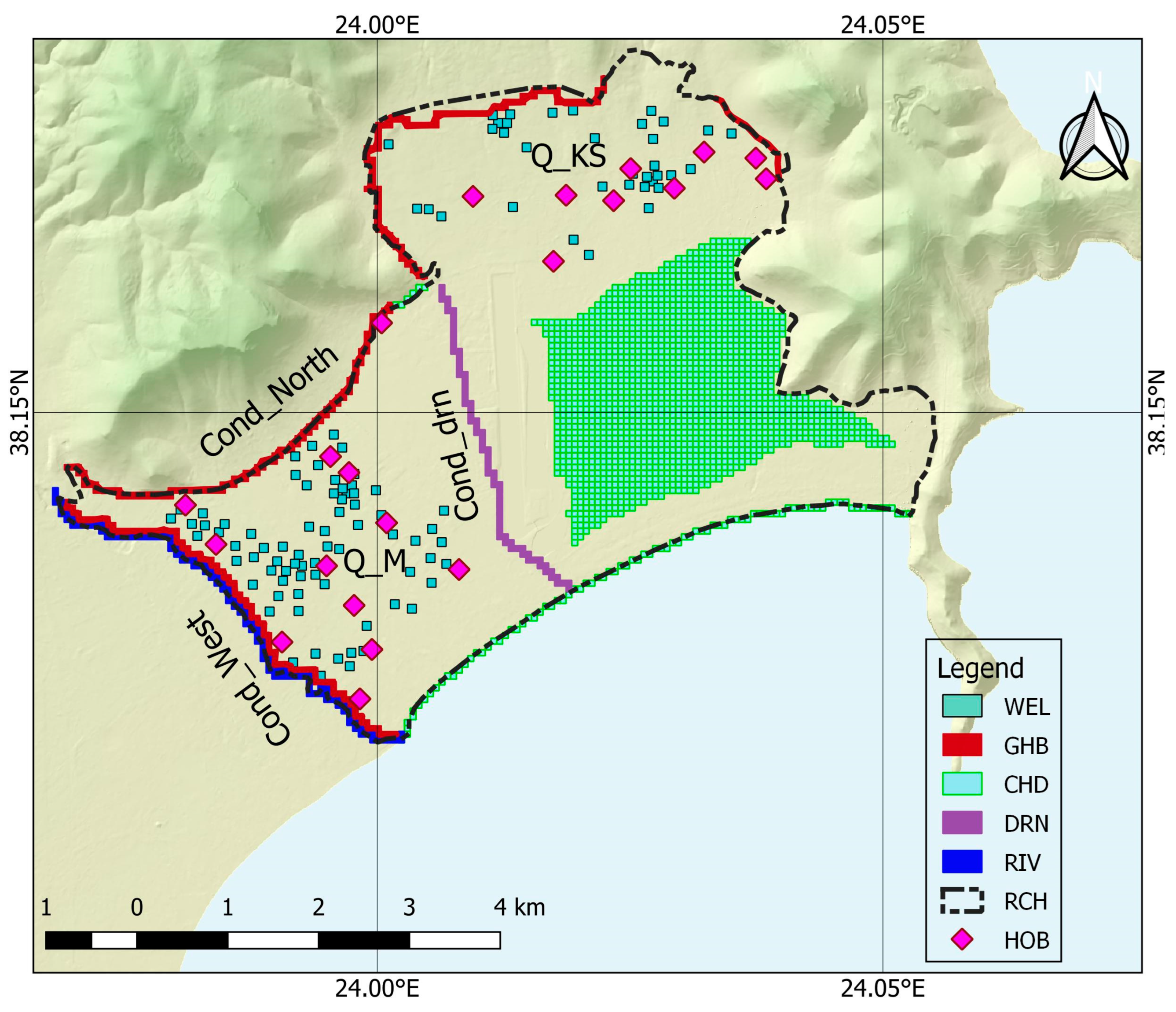
The major hydrologic compounds of the area are represented by different boundary conditions (Figure 2), as listed below and presented in Figure 5:
- 1.
- Dirichlet boundary conditions
- Coastline (Time-Variant Specified-Head package—CHD) at 0 m;
- Makaria Spring (Time-Variant Specified-Head package—CHD) at 2 m;
- Coastal Wetland (Time-Variant Specified-Head package—CHD) ranging from −1.2 m to 0.6 m to obtain observations in the vicinity of the wetland.
- 2.
- Neuman boundary conditions
- Abstraction wells and boreholes (Well package–WEL). Due to a lack of pumping rate data from the wells and drills, the pumping rate was determined based on data from the study of the Ministry of Agriculture [35] with an annual pumping rate of about 2 × 10⁶ m3;
- Percolation from precipitation (Recharge package—RCH). The distribution of rainwater percolation throughout the year was calculated through a model by employing different hydrological methods [38]. The model includes the Soil Conservation Service Curve Number (SCS-CN) approach [39], the Penman–Monteith method [40]) for Potential Evapotranspiration (PET), while the Soil Moisture Balance (SMB) [41] method was utilized to estimate the Actual Evapotranspiration and rainfall percolation in the aquifer.
- 3.
- Cauchy boundary conditions
- Inflows from the surrounding marble (General Head Boundary–GHB). For the boundary head of the GHB, several hydraulic head measurements were gathered during the field campaign (from October 2028 to September 2019). The hydraulic head of the karstic formation in the area varied from 2.5 m (during the dry season) up to 4 m (during the wet season);
- Drain canal (Drain package—DRN). For the elevation of the drain canal in the area, a Digital Elevation Model (DEM) was utilized.
- Haradros stream (River package—RIV). Since the stream has an ephemeral flow, a river stage of up to 1 m above the river bottom was utilized, according to the sparse observation data that were obtained during the field campaigns.
The Head Observation package (HOB) was also utilized in order to assign the observed values to the model.
Figure 5.
Model boundary conditions, sinks and sources.

To develop the variable density flow model, the MODFLOW and MT3DMS models were employed. The contaminant transport model was integrated into the flow model with common spatial and temporal discretization, enabling the Sink & Source Mixing Package (SSM). For the simulation, a type of pollutant was defined at the coastline as a constant concentration boundary condition representing the Mediterranean Sea. Initial conditions for the contaminant transport model were set from the chemical analysis data in terms of total dissolved solids (TDSs).
2.2.4. Parametrization
An important task during the conceptualization of a flow model is the determination of the type and value of the parameters and their spatial distribution. For the model of Marathon, parametrization was applied in order to define the parameters of the aquifers’ different zones and boundary conditions based on the collected data. Furthermore, the use of parameters is required for both the sensitivity analysis and calibration processes. In Table 1, the selected parameters for the aquifer of Marathon, as well as their initial values retrieved from past research [26,35,42], are presented.
3. Results
3.1. Sensitivity Analysis of MODFLOW Parameters
The results of the sensitivity analysis for the MODFLOW model were analyzed based on the CSS and PCC indices calculated by UCODE2014.
For the alluvial aquifer model, the results of the sensitivity analysis suggest that the model is highly influenced by the parameters related to the characteristics of the middle layer and sand–gravel zones, as well as the pumping parameters. The high values of the CSS index for the parameters HK2, SS_Par2, Q_KS and Q_M, as shown in Figure 6a, are partly due to the effect of pumping that takes place mainly in the middle layer formed entirely of sand–gravel. The specific yield (Sy) of the upper layer is less important for the simulation, while the parameters concerning the clay zones determine the result to an even lesser extent. The parameters concerning the boundary conditions and the model outputs (Cond_North, Cond_West and Cond_drn) have no significant sensitivity. A high correlation is observed between the Kato Souli pumping parameter (Q_KS) and the hydraulic properties of the sand–gravel (HK2, SS_Par2) and a smaller one with the Marathon pumping (Q_M) related to the effect of pumping on the middle layer, as described above and shown in Figure 6b.
3.2. MODFLOW Model Calibration and Results
Parameter estimation for the MODFLOW model was performed with respect to the sensitivity analysis results. The parameters selected for the UCODE2014 parameter estimation process concern the aquifer characteristics HK2, SS_Par2, Sy, HK1 and SS_Par1. The parameters Q_M and Q_KS were not included in the model calibration, and the initial values were used for the entire simulation. These parameters were primarily utilized to investigate the impact of withdrawals to the aquifer. The calibrated parameters are presented in the following table (Table 2).
The model improved significantly with respect to the measured hydraulic head after the calibration process. Furthermore, the statistics of the differences observed vs. the simulated hydraulic head, shown in Figure 7, present an acceptable agreement between the simulated and observed hydraulic head values.
3.3. Parameter Fitting in SEAWAT Model
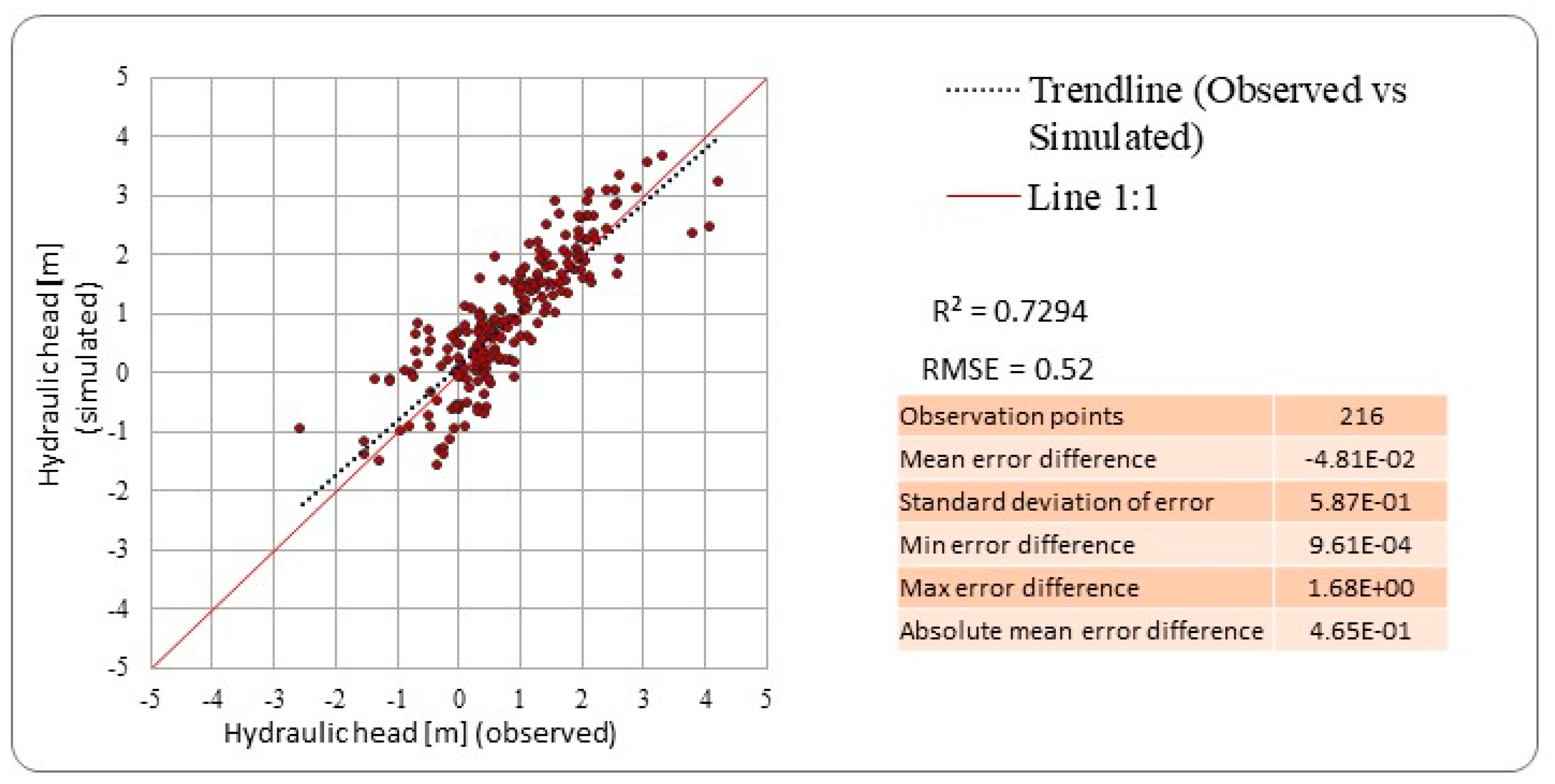
The parameters obtained from the MODFLOW-2005 calibration were used in the variable density flow model, SEAWAT. The Observation (OBS) Process, as described by Langevin et al. [43], was activated manually to test the fitting of the parameters in the SEAWAT model. The simulation results, in relation to the observed hydraulic head values, are presented in Figure 8. An acceptable agreement between the simulated and observed hydraulic head values was achieved in the SEAWAT model by utilizing the hydraulic parameters that were previously calibrated in the MODFLOW model. In fact, there is a slightly better match between the observed and simulated values with the SEAWAT model, as indicated by the metrics in Figure 8. The use of the SEAWAT model against the MODFLOW model in terms of the hydraulic head produced a greater match between the simulated and measured values and improved the results of the already calibrated flow model (MODFLOW-2005) without further calibration. The main difference between the two models is reflected in the near-the-shoreline observed vs. simulated values where the root-mean-square error (RMSE) is equal to 0.58 for the MODFLOW model, while for the SEAWAT model, the RMSE decreases to 0.50.
In addition, the simulation of the variable density flow model with the SEAWAT model produced different results in the distribution of the piezometric curves with respect to the MODFLOW model. The maps of iso-piezometric curves for the two models are presented in Figure 9 and Figure 10, for the simulated hydrological year (2018–2019). The main difference between the two models lies in the near-shoreline piezometric contours that are shifted further inland. This shift is due to the effect of the transition zone that cannot be captured by a non-variable density model. The difference between the two simulations is more pronounced during the period of extensive pumping, i.e., between July 2019 and September 2019.
Regarding the transport model parameters, no automatic calibration was performed due to the limited data. However, the manual calibration of longitudinal dispersivity and porosity was applied by assigning different parameter values utilized in the existing research [44,45,46,47,48,49]. The parameter calibration process revealed that no significant improvement in simulated–observed TDS values occurred. Nevertheless, there was an acceptable agreement between the observed vs. simulated TDS values (R2 = 0.9).
3.4. The Mechanism of Seawater Intrusion
In order to investigate further the mechanism of seawater intrusion in Marathon, the model was simulated for a longer period to achieve the natural mixing between the aquifer concentration and the seawater. The main goal was to investigate and determine the shape and the extent of the saltwater wedge in the coastal granular formation. According to Mabrouk et al. [50], two approaches are commonly used to determine the distribution of salinity in the aquifer: (a) assigning the initial salinity distribution spatially based on existing salinity data or (b) starting the simulation with a fully saline or fully freshwater aquifer and simulating for an extended period until the groundwater system reaches a dynamic equilibrium of a freshwater–seawater interface. Gomaa et al. [51], in their research in a coastal granular aquifer of Egypt, concluded that in the second case, freshwater occupied the development area, and the result did not match the salinity data. In contrast, the results of the first approach were in agreement with the observed values. Based on this conclusion and considering the existing salinity data, the first approach was adopted for the case of Marathon.
A reliable steady-state SEAWAT model was initially developed. To achieve steady-state conditions, the SEAWAT model was run for a “warm-up” period of 3000 timesteps. It must also be noted that the model was also run for a “warm-up” period of 10,000 timesteps, but the results revealed that steady-state conditions for the study area were achieved after 2000 timesteps. To this end, in order to reduce the computational burden, it was chosen to proceed with the modeling exercise using the initial model with the 3000 timesteps. The variable density flow was then simulated for 1827 timesteps under transient flow conditions for 5 hydrological years (2015–2020).
In Figure 11, cross-sections with the distribution of total dissolved solids (TDS) are plotted in the most affected areas of the aquifer as a result of the SEAWAT simulation.
In cross-section A-A’, a typical seawater intrusion wedge is formed. At this location, the extent of the freshwater–saltwater interface increases with depth toward inland. In the central part of the plain, the TDS concentration increases with depth up to 4 g/m3. The main cause of high TDS concentration is attributed to the cone of depression that appears during and after the dry period, a fact that is also validated by the chemical analysis and simulation results. During that season, extensive pumping led to upward movement of the freshwater–saltwater interface. The cone of depression is also validated by the hydraulic head in the area during the period of extensive pumping, i.e., from July to October (Figure 10). The upward movement of the interface is reflected in cross-section A-A as the TDS concentration is higher in the bottom layer (4 g/m3), and it is gradually decreased in the top layer (2.5 g/m3). Salinity is reduced toward the north where the karstic marble formation of lower salinity recharges the alluvial aquifer.
In cross-section B-B, the interface is moved further inland across the coastline, while in the northern part, the TDS concertation is lower than in cross-section A-A. The decrease in salinity is due to the seizing of groundwater withdrawals since the specific area is no longer cultivated.
Cross-section C-C presents the TDS concentration in the area of the wetland, where seawater intrusion extends further inland than in the western part of the plain. The extended transition zone is caused by the low topography of the wetland, as also stated by Margoni [37], in conjunction with the negative values of the hydraulic head that lower the hydraulic pressure in the aquifer, leading to extended seawater intrusion. In addition, the aquifer geological heterogeneity near the coastline (Figure 4) could have an effect on the extent and irregular shape of the transition zone.
4. Discussion
During the present research, an important issue arose related to the calibration process of the model since three different codes were implemented for the simulation of the coastal aquifer. Generally, for hydraulic parameter calibration, the MODFLOW model is utilized without taking into account the effects of the variable density flow that the SEAWAT code incorporates. Abd-Elaty and Zelenakova [47], in their research on the Nile Delta aquifer, calibrated the SEAWAT model with the trial-and-error method with respect to the TDS concentration. Ansarifar et al. [25] simulated the effect of sea level fluctuation with a calibrated MODFLOW model. Lyra et al. [24] utilized the MODFLOW model and PEST analysis to simulate and calibrate the hydraulic heads of a coastal aquifer, while solute transport parameters were calibrated through trial and error in the SEAWAT model. Nasiri et al. [52] in their research on seawater intrusion mitigation in coastal aquifers, calibrated hydraulic heads in the MODFLOW model and TDS concentration in the MT3DMS model before simulating the variable density flow with SEAWAT. In our research, the hydraulic heads were calibrated in the MODFLOW model and the TDS concentration in the SEAWAT model. In addition to methods used in the aforementioned studies, the OBS process was activated in the SEAWAT model [43]. This procedure revealed that the hydraulic parameters calibrated in MODFLOW produced better results for the observed vs. simulated head values of the SEAWAT model without further calibration by capturing the hydraulic head differences that the constant density flow model (MODFLOW) could not capture. Furthermore, this research reveals that the distribution of the hydraulic heads with SEAWAT differs from the piezometry produced by the MODFLOW model, especially in the areas of high TDS concentration (near the shoreline and at the wetland), where variable density effects are more pronounced. SEAWAT, the density-variant model, can be compared with MODFLOW, the density-invariant model, in which concentration or temperature changes do not affect the density. The results of the two cases are very similar or identical (Figure 7 and Figure 8) for the upstream part, where it can be observed that density is likely an insignificant part of the system behavior in that part of the two models. However, there is a significant difference between the two cases within the coastal zone, where it is proved that density is an important factor. As Post and Simmons [53] quote, the convective groundwater systems are mixed convection systems where forced convection (flow driven by pressure or hydraulic head gradients) and free convection (flow driven by density variations) co-exist.
As for the solute transport model parameters, in our case study, longitudinal dispersivity was of low importance for the TDS concentration, a result that is in accordance with Shoemaker’s research. Further validation of the model results can be carried out by obtaining hydraulic head and flow data near the coastline since effective locations for the calibration of SEAWAT with hydraulic head observations are the toe of the transition zone and areas near the coastline [54]. Unfortunately, during field research in the area, it was not possible to locate wells near the coastline, possibly due to the seizing of groundwater abstractions as a result of seawater intrusion. Furthermore, for the specific case study, the vertical discretization was decided with respect to the different hydrogeological zones of the alluvial aquifer, as indicated in Figure 4. Further vertical discretization would also improve the model. In order to apply vertical discretization and validate the produced results, an advanced research infrastructure (e.g., multilevel piezometers) is essential. As a result, this topic is reserved for future work.
Another outcome of the present research is the investigation of the seawater intrusion mechanism in the alluvial aquifer of Marathon. Considering the distribution and the shape of the hydraulic head in the aquifer (Figure 9 and Figure 10), the results of the simulation reveal that the aquifer is subjected to passive–active seawater intrusion, as analyzed by Werner [55]. In this situation, groundwater flows both inland and toward the sea. The phenomenon is more pronounced in the vicinity of the low-topography wetland, while at the central part of the plain, there is a temporal variability of the phenomenon. During the wet season, the hydraulic gradient is seaward, and a typical case of passive seawater intrusion occurs, while during the period of extensive pumping (July–October), the negative values of the hydraulic head increase the landward movement of seawater.
The extent and shape of the transition zone, as affected by the heterogeneity that characterizes the coastal formations, has been investigated through mathematical models by many researchers (e.g., refs. [56,57,58]), with the main conclusion that in heterogeneous porous formations, the freshwater–saltwater transition zone intensifies as a result of irregular flow conditions [1]. Across the wetland area, the transition zone does not form the typical saltwater wedge. In the middle layer of the aquifer, a much wider transition zone develops than in the lower layer, as it is affected by the different hydraulic properties of the aquifer’s zones. At the bottom layer, the zone of lower hydraulic conductivity (Figure 4c) prevents a faster development of seawater encroachment. The results are in accordance with Michael et al.’s [59] conclusion that geological heterogeneity has such a strong influence on the flow conditions that the salinity distribution and the shape of the freshwater–saltwater interface have an irregular and complex form, with no resemblance to the wedge-shaped interface consideration.
5. Conclusions
The present study involves the evaluation of variable density flow and assessment of the seawater intrusion mechanism in a coastal aquifer through modeling. The study area is a typical coastal Mediterranean hydrosystem located in Marathon, Greece.
The main conclusions derived from the use of MODFLOW and SEAWAT models to simulate groundwater flow are as follows: (i) the sensitivity analysis performed on the MODFLOW model with the UCODE_2014 code indicates that the most sensitive parameters are the hydraulic conductivity (HK) of the main aquifer layer (middle layer of the model), as well as the parameter of pumping (Q), concluding that the parameters related to the particular characteristics of the aquifer and the total water use (withdrawals) in the watershed have the greatest influence on the simulation of the aquifer, (ii) the use of the SEAWAT code to simulate flow under variable density conditions produced a greater match between the simulated and observed values of the hydraulic heads and, in this sense, further improved the results of the already calibrated flow model (MODFLOW-2005) and (iii) the distribution of hydraulic heads in the area produced with the MODFLOW model differ significantly with those produced with the SEAWAT model in the areas of high TDS concentration. Additionally, it appears that longitudinal dispersivity is not sensitive to the simulation. Regarding the “porosity” parameter, it appears that this parameter is more important for the simulation results in the variable density flow model than the “longitudinal dispersivity” parameter. However, the model results seem to be affected at very small porosity values (i.e., 0.05).
Parameter transferability seems to work, as even without calibration, the results of the SEAWAT model indicate a slightly better performance; thus, parameter transferability can take place between the two models. The limitations of this study lie in the lack of observed hydraulic head data near the coastline that would further validate the proposed framework since the most effective observation locations for the calibration of seawater intrusion models are those that are located near the coastline.
Finally, the mechanism of seawater intrusion in the area was assessed through the TDS concentration results produced from the SEAWAT model. The results indicate that the cone of depression at the central part of the plain is responsible for the high TDS concentration throughout the year. Furthermore, in the eastern part of the plain, the heterogeneity that characterizes the coastal formation in terms of the hydraulic parameters creates an irregular shape of the saltwater wedge in the specific area.
Author Contributions
Conceptualization, M.P., K.M. and A.K.; methodology, M.P., K.M. and A.K.; software, M.P., E.C., K.M. and A.K.; validation, M.P., E.C., K.M. and A.K.; formal analysis, M.P.; investigation, M.P., K.M. and A.K.; data curation, M.P.; writing—original draft preparation, M.P. and E.C.; writing—review and editing, M.P., E.C., K.M. and A.K.; visualization, M.P.; supervision, A.K. All authors have read and agreed to the published version of the manuscript.
Funding
This research was partially funded by the Special Account for Research Funding (E.L.K.E.) of the National Technical University of Athens (N.T.U.A.).
Data Availability Statement
The datasets generated and/or analyzed during the current study are available from the corresponding author upon reasonable request.
Acknowledgments
The authors would like to thank all the anonymous reviewers whose comments have greatly improved this manuscript.
Conflicts of Interest
The authors declare no conflicts of interest.
References
- Jiao, J.; Post, V. Coastal Hydrogeology; Cambridge University Press: Cambridge, UK, 2019; Volume 44, ISBN 9781139344142. [Google Scholar]
- Apostolopoulos, G.; Pouliaris, C.; Karizonis, S.; Perdikaki, M.; Kallioras, A. Integrated Analysis of the Coastal Aquifer System of Thorikos Valley, Attica, Greece. In Proceedings of the NSG2021 1st Conference on Hydrogeophysics, Bordeaux, France and Online, 29 August–2 September 2021; European Association of Geoscientists & Engineers: Utrecht, The Netherlands, 2021; pp. 1–5. [Google Scholar]
- Cosentino, P.; Capizzi, P.; Fiandaca, G.; Martorana, R.; Messina, P.; Pellerito, S. Study And Monitoring Of Salt Water Intrusion In The Coastal Area Between Mazara Del Vallo And Marsala (South-Western Sicily). In Methods and Tools for Drought Analysis and Management; Springer: Dordrecht, The Netherlands, 2007; pp. 303–321. [Google Scholar]
- Águila, J.F.; McDonnell, M.C.; Flynn, R.; Hamill, G.A.; Ruffell, A.; Benner, E.M.; Etsias, G.; Donohue, S. Characterizing Groundwater Salinity Patterns in a Coastal Sand Aquifer at Magilligan, Northern Ireland, Using Geophysical and Geotechnical Methods. Environ. Earth Sci. 2022, 81, 231. [Google Scholar] [CrossRef]
- Wilson, E.A.; Wells, A.J.; Hewitt, I.J.; Cenedese, C. The Dynamics of a Subglacial Salt Wedge. J. Fluid Mech. 2020, 895, A20. [Google Scholar] [CrossRef]
- Narayanan, D.; Eldho, T.I. Validation of Boundary Layer Solution for Assessing Mixing Zone Dynamics of Saltwater Wedge in a Coastal Aquifer. J. Hydrol. 2023, 617, 128899. [Google Scholar] [CrossRef]
- Torres-Bejarano, F.; González-Martínez, J.; Rodríguez-Pérez, J.; Rodríguez-Cuevas, C.; Mathis, T.J.; Tran, D.K. Characterization of Salt Wedge Intrusion Process in a Geographically Complex Microtidal Deltaic Estuarine System. J. S. Am. Earth Sci. 2023, 131, 104646. [Google Scholar] [CrossRef]
- Ke, S.; Chen, J.; Zheng, X. Influence of the Subsurface Physical Barrier on Nitrate Contamination and Seawater Intrusion in an Unconfined Aquifer. Environ. Pollut. 2021, 284, 117528. [Google Scholar] [CrossRef] [PubMed]
- Dokou, Z.; Karatzas, G.P. Saltwater Intrusion Estimation in a Karstified Coastal System Using Density-Dependent Modelling and Comparison with the Sharp-Interface Approach. Hydrol. Sci. J. 2012, 57, 985–999. [Google Scholar] [CrossRef]
- Diersch, H.-J.G. FEFLOW; Springer: Berlin/Heidelberg, Germany, 2014; Volume 9783642387, ISBN 978-3-642-38738-8. [Google Scholar]
- Stoeckl, L.; Walther, M.; Morgan, L.K. Physical and Numerical Modelling of Post-Pumping Seawater Intrusion. Geofluids 2019, 2019, 7191370. [Google Scholar] [CrossRef]
- Na, J.; Chi, B.; Zhang, Y.; Li, J.; Jiang, X. Study on the Influence of Seawater Density Variation on Sea Water Intrusion in Confined Coastal Aquifers. Environ. Earth Sci. 2019, 78, 669. [Google Scholar] [CrossRef]
- Xu, T.; Sonnenthal, E.; Spycher, N.; Pruess, K. TOUGHREACT User’s Guide: A Simulation Program for Non-Isothermal Multiphase Reactive Geochemical Transport in Variably Saturated Geologic Media, V1.2.1; Lawrence Berkeley National Laboratory: Berkeley, CA, USA, 2008. [Google Scholar]
- Langevin, C.D.; Thorne, D.T., Jr.; Dausman, A.M.; Sukop, M.C.; Guo, W. SEAWAT Version 4: A Computer Program for Simulation of Multi-Species Solute and Heat Transport; U.S. Geological Survey Techniques and Methods Book 6; U.S. Geological Survey: Reston, VA, USA, 2007; 39p.
- Dunlop, G.; Palanichamy, J.; Kokkat, A.; EJ, J.; Palani, S. Simulation of Saltwater Intrusion into Coastal Aquifer of Nagapattinam in the Lower Cauvery Basin Using SEAWAT. Groundw. Sustain. Dev. 2019, 8, 294–301. [Google Scholar] [CrossRef]
- Abd-Elhamid, H.F.; Abd-Elaty, I.; Sherif, M.M. Effects of Aquifer Bed Slope and Sea Level on Saltwater Intrusion in Coastal Aquifers. Hydrology 2019, 7, 5. [Google Scholar] [CrossRef]
- Gopinath, S.; Srinivasamoorthy, K.; Saravanan, K.; Prakash, R.; Karunanidhi, D. Characterizing Groundwater Quality and Seawater Intrusion in Coastal Aquifers of Nagapattinam and Karaikal, South India Using Hydrogeochemistry and Modeling Techniques. Hum. Ecol. Risk Assess. Int. J. 2019, 25, 314–334. [Google Scholar] [CrossRef]
- Harbaugh, A.W. MODFLOW-2005, The U.S. Geological Survey Modular Ground-Water Model—The Ground-Water Flow Process; U.S. Geological Survey Techniques and Methods; U.S. Geological Survey: Reston, VA, USA, 2005; p. 253. ISBN 6-A16.
- Zheng, C.; Wang, P. MT3DMS: A Modular Three-Dimensional Multispecies Transport Model for Simulation of Advection, Dispersion, and Chemical Reactions of Contaminants in Groundwater Systems Documentation and User ’s Guide; US Army Engineer Research and Development Center: Vicksburg, MS, USA, 1999. [Google Scholar]
- Akhtar, J.; Sana, A.; Tauseef, S.M.; Tanaka, H. Numerical Modeling of Seawater Intrusion in Wadi Al-Jizi Coastal Aquifer in the Sultanate of Oman. Hydrology 2022, 9, 211. [Google Scholar] [CrossRef]
- Chang, S.W.; Clement, T.P. Experimental and Numerical Investigation of Saltwater Intrusion Dynamics in Flux-controlled Groundwater Systems. Water Resour. Res. 2012, 48, W09527. [Google Scholar] [CrossRef]
- Khadim, F.K.; Dokou, Z.; Lazin, R.; Moges, S.; Bagtzoglou, A.C.; Anagnostou, E. Groundwater Modeling in Data Scarce Aquifers: The Case of Gilgel-Abay, Upper Blue Nile, Ethiopia. J. Hydrol. 2020, 590, 125214. [Google Scholar] [CrossRef]
- Carrera, J.; Hidalgo, J.J.; Slooten, L.J.; Vázquez-Suñé, E. Computational and Conceptual Issues in the Calibration of Seawater Intrusion Models. Hydrogeol. J. 2010, 18, 131–145. [Google Scholar] [CrossRef]
- Lyra, A.; Loukas, A.; Sidiropoulos, P.; Tziatzios, G.; Mylopoulos, N. An Integrated Modeling System for the Evaluation of Water Resources in Coastal Agricultural Watersheds: Application in Almyros Basin, Thessaly, Greece. Water 2021, 13, 268. [Google Scholar] [CrossRef]
- Ansarifar, M.-M.; Salarijazi, M.; Ghorbani, K.; Kaboli, A.-R. Simulation of Groundwater Level in a Coastal Aquifer. Mar. Georesources Geotechnol. 2020, 38, 257–265. [Google Scholar] [CrossRef]
- Perdikaki, M.; Makropoulos, C.; Kallioras, A. Participatory Groundwater Modeling for Managed Aquifer Recharge as a Tool for Water Resources Management of a Coastal Aquifer in Greece. Hydrogeol. J. 2022, 30, 37–58. [Google Scholar] [CrossRef]
- Psychoyou, M.; Mimides, T.; Rizos, S.; Sgoubopoulou, A. Groundwater Hydrochemistry at Balkan Coastal Plains—The Case of Marathon of Attica, Greece. Desalination 2007, 213, 230–237. [Google Scholar] [CrossRef]
- Perdikaki, M.; Manjarrez, R.C.; Pouliaris, C.; Rossetto, R.; Kallioras, A. Free and Open-Source GIS-Integrated Hydrogeological Analysis Tool: An Application for Coastal Aquifer Systems. Environ. Earth Sci. 2020, 79, 16. [Google Scholar] [CrossRef]
- Harbaugh, B.A.W.; Banta, E.R.; Hill, M.C.; Mcdonald, M.G. MODFLOW-2000, The U.S. Geological Survey Modular Graound-Water Model—User Guide to Modularization Concepts and the Ground-Water Flow Process; U.S. Geological Survey: Reston, VA, USA, 2000; p. 130.
- Winston, R.B. ModelMuse: A Graphical User Interface for MODFLOW-2005 and PHAST; U.S. Geological Survey Techniques and Methods 6–A29; U.S. Geological Survey: Reston, VA, USA, 2009; p. 52.
- Perdikaki, M. Modelling and Optimized Management in Coastal Aquifer Systems; National Technical University of Athens: Athens, Greece, 2022. [Google Scholar]
- Poeter, E.P.; Hill, M.C.; Lu, D.; Tiedeman, C.R.; Mehl, S. UCODE_2014, with New Capabilities to Define Parameters Unique to Predict Ions, Calculate Weights Using Simulated Values, Estimate Parameters with SVD, Evaluate Uncertainty with MCMC, and More; Integrated Groundwater Modeling Center (IGWMC), of the Colorado School of Mines: Golden, CO, USA, 2014. [Google Scholar]
- Banta, E.R. ModelMate—A Graphical User Interface for Model Analysis. In Techniques and Methods 6–E4; U.S. Geological Survey: Reston, VA, USA, 2000. [Google Scholar]
- Poeter, E.; Hill, M.; Banta, E.; Mehl, S.; Christensen, S. UCODE 2005 and Six Other Computer Codes for Universal Sensitivity Analysis, Calibration, and Uncertainty Evaluation; U.S. Geological Survey: Reston, VA, USA, 2005. [Google Scholar]
- Melissaris, P.; Stavropoulos, X. Hydrogeological Study of the Marathon Plain, Atticaq; Ministry of Agricultural Development: Department of Geology–Hydrogeology: Athens, Greece, 1999. [Google Scholar]
- Margoni, S. Research of the Environmental Evolution Processes of the Wetlands and Plain of Marathon during the Holocene with the Use of Geographic Information Systems; Aristotle University of Thessaloniki: Thessaloniki, Greece, 2006. [Google Scholar]
- Lozios, S. Tectonic Analysis of the Metamorphic Units of Northeastern Attica; National and Kapodistrian University of Athens: Athens, Greece, 1994. [Google Scholar]
- Perdikaki, M.; Kallioras, A. Estimating Groundwater Recharge from Precipitation in a Coastal Mediterranean Aquifer: The Case of Marathon. In Proceedings of the 12th World Congress of EWRA on Water Resources and Environment, Thessaloniki, Greece, 27 June–1 July 2023. [Google Scholar]
- Mckeever, V.; Owen, W.; Rallison, R.; Engineers, H. National Engineering Handbook Section 4—Hydrology; Soil Conservation Service: 1972. Available online: https://docslib.org/doc/4839451/national-engineering-handbook-section-4-hydrology (accessed on 22 January 2024).
- Allen, R. Penman–Monteith Equation. In Encyclopedia of Soils in the Environment; Elsevier: Amsterdam, The Netherlands, 2005; Volume 4, pp. 180–188. [Google Scholar]
- Thornthwaite, C.W.; Mather, J.R. Instructions and Tables for Computing Potential Evapotranspiration and the Water Balance. Drexel Institute of Technology. Laboratory of Climatology. Publ. Climatol. 1957, 10, 181–289. [Google Scholar]
- Siemos, N. Evaluation of Water Resources in Attica and Islands of Argosaronic Gulf; Institute of Geology and Mineral Exploration: Athens, Greece, 2010. [Google Scholar]
- Langevin, C.D.; Shoemaker, W.B.; Guo, W. MODFLOW-2000, the U.S. Geological Survey Modular Ground-Water Model-Documentation of the SEAWAT-2000 Version with the Variable-Density Flow Process (VDF) and the Integrated MT3DMS Transport Process (IMT); U.S. Geological Survey: Reston, VA, USA, 2003.
- Gelhar, L.W.; Welty, C.; Rehfeldt, K.R. A Critical Review of Data on Field-Scale Dispersion in Aquifers. Water Resour. Res. 1992, 28, 1955–1974. [Google Scholar] [CrossRef]
- Schulze-Makuch, D. Longitudinal Dispersivity Data and Implications for Scaling Behavior. GroundWater 2005, 43, 443–456. [Google Scholar] [CrossRef] [PubMed]
- Oude Essink, G.H.P.; Van Baaren, E.S.; De Louw, P.G.B. Effects of Climate Change on Coastal Groundwater Systems: A Modeling Study in the Netherlands. Water Resour. Res. 2010, 46, W00F04. [Google Scholar] [CrossRef]
- Abd-Elaty, I.; Zelenakova, M. Saltwater Intrusion Management in Shallow and Deep Coastal Aquifers for High Aridity Regions. J. Hydrol. Reg. Stud. 2022, 40, 101026. [Google Scholar] [CrossRef]
- Tran, D.A.; Tsujimura, M.; Pham, H.V.; Nguyen, T.V.; Ho, L.H.; Le Vo, P.; Ha, K.Q.; Dang, T.D.; Van Binh, D.; Doan, Q.-V. Intensified Salinity Intrusion in Coastal Aquifers Due to Groundwater Overextraction: A Case Study in the Mekong Delta, Vietnam. Environ. Sci. Pollut. Res. 2022, 29, 8996–9010. [Google Scholar] [CrossRef] [PubMed]
- Siarkos, I. Developing a Methodological Framework Using Mathematical Simulation Models in Order to Investigate the Operation of Coastal Aquifer Systems: Application in the Aquifer of N. Moudania; Aristotle University of Thessaloniki, School of Civil Engineering: Thessaloniki, Greece, 2015. [Google Scholar]
- Mabrouk, M.; Jonoski, A.; Oude Essink, G.; Uhlenbrook, S. Assessing the Fresh–Saline Groundwater Distribution in the Nile Delta Aquifer Using a 3D Variable-Density Groundwater Flow Model. Water 2019, 11, 1946. [Google Scholar] [CrossRef]
- Gomaa, S.M.; Hassan, T.M.; Helal, E. Assessment of Seawater Intrusion under Different Pumping Scenarios in Moghra Aquifer, Egypt. Sci. Total Environ. 2021, 781, 146710. [Google Scholar] [CrossRef]
- Nasiri, M.; Moghaddam, H.K.; Hamidi, M. Development of Multi-Criteria Decision Making Methods for Reduction of Seawater Intrusion in Coastal Aquifers Using SEAWAT Code. J. Contam. Hydrol. 2021, 242, 103848. [Google Scholar] [CrossRef]
- Post, V.; Simmons, C. Variable Density Groundwater Flow; The Groundwater Project: Guelph, ON, Canada, 2022; ISBN 9781774700464. [Google Scholar]
- Shoemaker, W.B. Important Observations and Parameters. GroundWater 2004, 42, 829–840. [Google Scholar]
- Werner, A.D. On the Classification of Seawater Intrusion. J. Hydrol. 2017, 551, 619–631. [Google Scholar] [CrossRef]
- Abarca, E.; Vázquez-Suñé, E.; Carrera, J.; Capino, B.; Gámez, D.; Batlle, F. Optimal Design of Measures to Correct Seawater Intrusion. Water Resour. Res. 2006, 42, W09415. [Google Scholar] [CrossRef]
- Kerrou, J.; Renard, P. A Numerical Analysis of Dimensionality and Heterogeneity Effects on Advective Dispersive Seawater Intrusion Processes. Hydrogeol. J. 2010, 18, 55–72. [Google Scholar] [CrossRef]
- Pool, M.; Post, V.E.A.; Simmons, C.T. Effects of Tidal Fluctuations and Spatial Heterogeneity on Mixing and Spreading in Spatially Heterogeneous Coastal Aquifers. Water Resour. Res. 2015, 51, 1570–1585. [Google Scholar] [CrossRef]
- Michael, H.A.; Scott, K.C.; Koneshloo, M.; Yu, X.; Khan, M.R.; Li, K. Geologic Influence on Groundwater Salinity Drives Large Seawater Circulation through the Continental Shelf. Geophys. Res. Lett. 2016, 43, 10782–10791. [Google Scholar] [CrossRef]
Figure 1.
Methodological framework.

Figure 2.
Study area—Marathon hydrosystem, with a hydrogeological cross-section.

Figure 3.
TDS concentration in Marathon Plain.

Figure 4.
Layer zonation in the (a) upper aquifer layer, (b) middle aquifer layer and (c) lower aquifer layer.
Figure 4.
Layer zonation in the (a) upper aquifer layer, (b) middle aquifer layer and (c) lower aquifer layer.

Figure 6.
Sensitivity analysis results: (a) Composite Scaled Sensitivities—CSS; (b) Parameter Correlation Coefficient—PCC.
Figure 6.
Sensitivity analysis results: (a) Composite Scaled Sensitivities—CSS; (b) Parameter Correlation Coefficient—PCC.

Figure 7.
Observed vs. simulated hydraulic head values for the MODFLOW model.

Figure 8.
Observed vs. simulated hydraulic head values for the SEAWAT model.

Figure 9.
MODFLOW vs. SEAWAT hydraulic head in meters—wet season.

Figure 10.
MODFLOW vs. SEAWAT hydraulic head in meters—dry season.

Figure 11.
Aquifer TDS concentration in cross-section as a result of SEAWAT model.


Table 1.
Model parameters.
| Parameter | Parameter Name | Initial Value |
|---|---|---|
| Hydraulic conductivity of clay zone | HK1 | 0.2 (m/day) |
| Hydraulic conductivity of sand–gravel zone | HK2 | 3.312 (m/day) |
| Specific yield for the upper layer | Sy | 0.02 |
| Conductance of the northern GHB boundary (marble) | Cond_North | 32210 (m2/day) |
| Conductance of the western GHB boundary (adjacent aquifer) | Cond_West | 7395.8 (m2/day) |
| Conductance of the DRN boundary | Cond_drn | 8.64 (m2/day) |
| Specific storage of clay zone | SS_Par1 | 8.24E−3 (m−1) |
| Specific storage of sand–gravel zone | SS_Par2 | 8.24E−3 (m−1) |
| Pumping rate (WEL package) at the W of the plain | Q_M | −60 (m3/day) |
| Pumping rate (WEL package) at the NE of the plain | Q_KS | −170 (m3/day) |
Table 2.
Parameter estimation results.
| Parameter | Calibrated Value |
|---|---|
| HK2 | 12.92 (m/day) |
| SS_Par2 | 7.79E−05 (m−1) |
| SY | 0.03927 |
| HK1 | 0.8061 (m/day) |
| SS_Par1 | 0.000542 (m−1) |
Disclaimer/Publisher’s Note: The statements, opinions and data contained in all publications are solely those of the individual author(s) and contributor(s) and not of MDPI and/or the editor(s). MDPI and/or the editor(s) disclaim responsibility for any injury to people or property resulting from any ideas, methods, instructions or products referred to in the content. |
© 2024 by the authors. Licensee MDPI, Basel, Switzerland. This article is an open access article distributed under the terms and conditions of the Creative Commons Attribution (CC BY) license (https://creativecommons.org/licenses/by/4.0/).
Share and Cite
MDPI and ACS Style
Perdikaki, M.; Chrysanthopoulos, E.; Markantonis, K.; Kallioras, A. Groundwater Flow Model Calibration Using Variable Density Modeling for Coastal Aquifer Management. Hydrology 2024, 11, 59. https://doi.org/10.3390/hydrology11040059
AMA Style
Perdikaki M, Chrysanthopoulos E, Markantonis K, Kallioras A. Groundwater Flow Model Calibration Using Variable Density Modeling for Coastal Aquifer Management. Hydrology. 2024; 11(4):59. https://doi.org/10.3390/hydrology11040059
Chicago/Turabian StylePerdikaki, Martha, Efthymios Chrysanthopoulos, Konstantinos Markantonis, and Andreas Kallioras. 2024. "Groundwater Flow Model Calibration Using Variable Density Modeling for Coastal Aquifer Management" Hydrology 11, no. 4: 59. https://doi.org/10.3390/hydrology11040059
Note that from the first issue of 2016, this journal uses article numbers instead of page numbers. See further details here.