Evaluation of Multiresolution Digital Elevation Model (DEM) from Real-Time Kinematic GPS and Ancillary Data for Reservoir Storage Capacity Estimation

Abstract

This study presents the estimation of reservoir storage capacity using multiresolution Real-Time Kinematic Global Positioning System (RTK-GPS) DEM, in comparison with ASTER and contour-derived DEM. Through RMSE comparisons of the elevation point uncertainty and error analysis, the results shows that the RTK-GPS DEM gave the best results for the reservoir capacity-area power curve estimation, defined by a convex slope with an exponential deterministic relationship given by $V=0.09\times A^{1.435}$. The results further show the existence an empirical relationship between the reservoir volume certainty and the GPS point density $d_i$ as $V_e=c\times d_i^{\rho }$. This relationship is dependent on the reservoir terrain, slope and surface area. Validation of the results with in situ data showed the differences between the simulated and observed storage volumes was less than +10%, and using the Nash-Sutcliffe coefficient of efficiency on the storage volumes, an average efficiency of +0.7 on the monthly observed and simulated reservoir storage volume was observed.

1. Introduction

With the variations of spatial-temporal distributions of runoff due in part to climate change, small reservoirs for water detention will continue to serve multipurpose uses including water supply, flood control, hydropower generation, navigation and recreation [1,2,3]. In this study, small-reservoirs are defined as those reservoirs storing less than one-million cubic meters of water, and are often used to capture and retain runoff water in the form of shallow lakes, wetlands or ephemeral ponds.

In the planning and maintenance of such structures, relationships between a reservoir’s surface area A, storage capacity or volume V, and the depth D of water, are significant in the evaluation of water and dissolved-mass balances of the reservoir system. The correlations amongst these reservoir parameters are equally significant in real-time and long-term monitoring of such water detention systems. Conventionally, reservoir characterization parameters and relationships such as A-D and V-D are often determined from fine-resolution topographical maps that are derived from detailed engineering surveys [4]. Such conventional methods are however time-consuming, field laborious and subject to observational errors.

As an alternative to topographic maps, the planning, design, construction and monitoring of reservoirs can automatically be accomplished through generation and analysis of digital elevation models (DEMs). Laser and LiDAR scanning techniques can now furnish guided results for 3Dcloud data acquisition of medium to high-resolution “bare-earth” DEM [5,6]. The authors of [7] concluded that every data source and method for reservoir storage analysis have their advantages and limitations, which can be attributed to the availability of data, reservoir size and location, among other variables. The exploration of modern data acquisition techniques should, however, be coupled with the development of suitable methods for reservoir capacity information derivation.

Because the spatial resolution of digital elevation model has a significant influence on the accuracy of reservoir storage estimation curves [7], it is desirable to use a higher resolution and more accurate DEMs. Real-Time Kinematic surveys using the Global Positioning Systems (RTK-GPS) can provide quick, cheaper and high-resolution data for terrain DEM representation [8], as has been used in reservoir water and underwater bathymetric surveys [9,10]. RTK-GPS, like LiDAR can also be used to create “bare-earth” elevation model that is free of man-made and natural features in the DEM representation. The only difference might be in the data capture and processing efficacy, and in the data quality and time-cost factors in the acquisitions of required data.

Based on the advantages of the RTK-GPS, the rationale of the current study is that using the near pinpoint accuracy provided by RTK-GPS with ground augmentations, accurate topographic DEM information can rapidly be obtained thereby significantly reducing the amount of time and labor that is normally required when conventional methods in determining the fundamental reservoir hydrologic characteristics.

Despite the applicability of DEM data, the spatially varying complexity of actual topography and its strongly anisotropic (or directional) behavior preclude a straightforward analytical approach to the interpolation of elevation DEM. These difficulties can be addressed with analytical methods, by dividing the region into small adjoining pieces, but problems remain in deciding the size of such pieces, how to join them together and how to address anisotropic behavior still within, and immediately beyond each piece.

To address these shortfalls and explore the potentials of RTK-GPS derived DEM, the objectives of the current study are four-fold: (i) set up an uncertainty and error analysis to optimize and define the optimal RTK-GPS point density for a given terrain case study through simulated comparative evaluation; (ii) compare the RTK-GPS results with ASTER Global DEM (ASTERGDEM) and planimetric (contour) interpolated DEM in order to understand the influence of point density distribution and interpolation on the reliability of gridded DEM; and (iii) apply the DEM sampling scheme from the results above to derive the reservoir surface hydrologic parameters, and compare the results with fitted reservoir storage capacity relationships as: A-D, V-D and V-A that are specific to a given site, but are important in the reservoir capacity monitoring once in operation; (iv) To compute the area of the reservoir, a modified reservoir area computation approach using surface to horizontal area ratio concept is proposed in this study and compared with the conventional GIS-based methods.

The rest of the paper is organized as follows: the second section presents a review on the conventional methods for reservoir storage capacity estimations, followed by a brief on the study area description. Section 4 is on RTK-GPS theory, and on the principles of DEM generation and uncertainty-error analysis with test results. The fifth and sixth sections of the paper respectively presents the methodological approaches for determination of the reservoir geometric characteristics using RTK-GPS DEM in comparison with ASTERGDEM and contour generated DEMs, and the model validation results. The study discussions, conclusions and recommendations are respectively presented in sections seven and eight.

2. Brief Review on Reservoir Storage Capacity Estimation

The traditionally used methods for reservoir capacity estimation depict a reservoir as presented in Figure 1. Using direct computational methods, the storage volume is estimated from the reservoir width, the throwback, and maximum impounded water depth [11]. Due to the complexities involved in deriving these reservoir geometric elements, most small-reservoirs are often constructed without considering the requisite topographic and or surface spatial information.

The direct methods for estimating small-reservoir storage capacities are based on the defined and measured dimensions as depicted in Figure 1a. These spatial elements are connected mathematically according to Equation (1) [12,13].

$$V=k\times D\times W\times T$$

(1)

where: k is a constant related to the size of the valley cross-section and dam length; D is the maximum water depth (m), i.e., difference in elevation between the dam at the spillway crest level); W is the width (m) of water surface at the spillway crest level, and T is the throwback at the spillway crest level (m), i.e., distance from the dam wall along the reservoir axis usually to the point where river enters.

The constant k varies according to the geometric size of the reservoir and was formulated by [12], with varying reservoir results as shown in Figure 1b. Figure 1b shows that a higher k value corresponds to higher surface area A and subsequently to a higher reservoir capacity V. The variations in V-A-D is schematically depicted in Figure 1a, where the change in water level $(\Delta z=\Delta D)$ is defined by the differences in elevation $(\Delta \mathrm{z}={\mathrm{Z}}_{\mathrm{i}+1}-{\text{ Z}}_{\mathrm{i}})$.

If the reservoir surface is of an unusual shape, Equation (2) is used to provide a better capacity estimate. In Equation (2), the constant $k_1$ related to the shape of the reservoir is introduced. Previous studies by [4] and [14] showed that the value of $k_1$ ranges between 0–1, while $k_2$ (a factor related to reservoir sizes) values are typically above 0.5.

$$V=k_1\times k_2\times D\times W\times T$$

(2)

To improve on the traditional-direct reservoir parameter estimation methods, either the mid-area (Equation (3)) or the prismoidal (Equation (4)) [12] formulae for volume computations can be used.

$$V={\displaystyle \sum _{i=1}^n\left(\frac{A_i+A_{i+1}}{2}\right)\times \Delta z}$$

(3)

$$V={\displaystyle \sum _{i=1}^n\left\{\Delta z\times \left[A_i+\left(\sqrt{A_i+A_{i+1}}\right)+A_{i+1}\right]/3\right\}}$$

(4)

where: $A_i$ = surface area at contour interval ${\mathrm{Z}}_{\mathrm{i}}$; $A_{i+1}$ = surface area at the next contour level above contour level $Z_{i+1}$ and $\Delta z$ is the corresponding contour interval. From Equations (3) and (4), the storage $V_{i+1}$ at level $Z_{i+1}$ can be defined by the expression $V_{i+1}={\displaystyle \sum _{k=0}^i{\nu }_{k+1}}$.

The mid-area formula assumes that the areas contained within successive contours represent cross-sections $Z_i$ and $Z_{i+1}$, and the distances between the respective contours is the contour interval $(\Delta z)$. The prismoidal method on the other hand assumes that the capacity enclosed by two contour intervals represents a prism. With respect to accuracy, the mid-area method is more suitable where the contour interval $(\Delta z)$ is small.

Figure 1b implies that within a geomorphologically homogenous region, a good correlation between the reservoir’s surface area and the capacity is expected. Such a correlation however depends on the general shape of the slopes (convex, through straight, to concave). For straight slopes, the reservoir is expected to have the shape of half a pyramid, with the dam forming the base of the (half) pyramid. For such straight slopes, it is expected that the volume will depend on the area to the power of one and a half, as depicted in the deterministic V-A function (Equation (5)). In reality, however, slopes tend to be convex, resulting in the power relationship being less than the exponent of 1.5, hence triangular reservoirs.

$$\mathrm{V}=\text{k}\times {\mathrm{A}}^{1.5}$$

(5)

Besides the direct methods, indirect methods for estimating surface areas from remote sensing imaging and Global Positioning Systems (GPS) can also be adopted. While the former has been investigated, e.g., [12,15], the latter has not been investigated due to the initially low vertical and positional accuracies [16,17].

Table 1. Summary of literature review on reservoir storage capacity estimations and geometric analysis from digital elevation model (DEM) and related studies.

Study/Reference	Data Used/Data Compared	Location/Number of Test Sites	Reservoir Parameters Derived from DEM	Study Approach, Result(s) and Recommendations
Magome et al. [7,11]	LandSat data DEM from GTOPO30 Lake water levels from altimetry data	Yagisawa Reservoir in Japan (2002) and Akosombo dam in Ghana (2003)	Area-Volume (A–V) curve, Height or Depth-Volume (H–V) and Height-Area (H–A) relationships	Multiemporal monitoring of seasonal and interannual variation of water storage of the reservoirs Estimated the reservoir storage capacity using remote sensing data and DEM for ungauged basins Resolution of DEM influences the accuracy of storage power curves, and recommended higher spatial resolution DEM
Peng et al. [12]	LandSat data Topographic maps Hydrographic surveys	Fengman reservoir basin in China	No application of DEM	Use of LandSat data in reservoir surface area determination yielded similar results to the traditional approach Used 4th order polynomial to determine a new storage curve for the reservoir
Vaze et al. [19]	LiDAR and contour map used to derived DEM with a resolution of 25 m	NSW Australia in the Koondrook–Perricoota forest area	Multigrid DEM of 1 m, 2 m, 5 m, 10 m and 25 m resolutions	DEM accuracy and resolution impacts on the quality of topographic indices The quality of DEM-derived hydrological features is sensitive to both DEM accuracy and DEM grid size (resolution)
Venkatesan et al. [20]	Topographical maps 90 m DEM from SRTM Differential GPS	14 small tanks (reservoirs) in the Sindapalli Uppodai sub-basin, Tamil Nadu, India	90 m SRTM DEM used to derive the reservoir capacity	Reservoir surface area determination using DGPS Water surface area-storage capacity relationship using log capacity-area approach
Lee [21]	LiDAR Multibeam echo sounders KTK-GPS	Randy Poynter Lake in Rockdale County, Georgia	Multisource and multiresolution DEM combined for 3D reservoir model generation	The datasets combined to create a 3D model of the reservoir for the generation of a stage-storage curve. Accurate 3D model of the lake provides the storage capacity used to establish a baseline for monitoring future sedimentation
Zhang and Chu [18]	Physical and simulated watershed surface	Simulated DEM and case study of smooth and mountainous areas	Multiple DEM grid spacing (20 m–500 m) and effect on surface topographic detail representation and volume computation	DEMs and their accuracy depend on their resolutions or grid sizes, the acquisition technologies, sources of the original data and interpolation/aggregation methods). Recommended use of LiDAR for high-accuracy and high-resolution DEMs
Current study	DEM from RTK-GPS ASTER Global DEM Topographic map contours	Kesses reservoir in Kenya	Multi-grid DEM analysis at 0.1 m, 1 m, 3 m, 10 m, 30 m, 90 m resolutions Elevation, slope and surface area	From the above literature surveys, there is demand for higher resolution and more accurate DEM. The following are the contributions of the current study: Method for estimating potential reservoir storage capacity based on higher resolution and accurate DEM using RTK-GPS. Only two studies [20,21] respectively used DGPS and RTK-GPS A derivation of the relationship between the reservoir storage elements (volume-area-depth (V-A-D))for the proposed reservoir Useful in normal terrain in areas with scarce gauge data The quality of DEM-derived hydrologic features is sensitive to both DEM accuracy and DEM grid size, and a relationship between capacity and grid density is established for the case study

presents a summary of related studies on the estimation and monitoring of reservoir storage capacities. From the literature review, the following conclusions are made: (i) initial studies on DEM based reservoir capacity estimation using non-traditional methods (e.g., [7,11,12] observed that the accuracy of DEMs significantly influences the accuracy of reservoir storage estimation curves. As such it is desirable to use higher resolution and more accurate DEMs in reservoir storage capacity estimations; (ii) Most of the studies have concentrated on the development of reservoir storage capacities using remote sensing data for monitoring existing reservoirs, and not on the development of the potential storage capacities for proposed reservoirs; (iii) Most of the case studies that utilized DEMs relied on either topographical map contours or on coarse resolution 90 m DEM from Shuttle Radar Topography Mission (SRTM) or Advanced spaceborne Thermal Emission and Reflection Radiometer (ASTER). The studies recommended the use of high resolution DEMs and also the determination of the optimal DEM resolution or grid size for higher accuracy in reservoir capacity estimations; (iv) [18,19] emphasized on the influence of terrain variations in reservoir storage capacity estimations and on multigrid analysis respectively for general terrain DEM analysis, with [19,20,21] utilizing LiDAR, Differential GPS (DGPS) and RTK-GPS for reservoir elevation derivations.

GPS observations allows for the collection of spatially-distributed 3D coordinates, from which the surface digital terrain modelling (DTM) of a reservoir can be derived. Terrain attributes can then be readily estimated from GPS-derived DEMs, and depends on the accuracy with the DEM represents the terrain. Using the results of the high-accuracy GPS surveys, high-resolution DEMs can be derived as the observational grid network can be set out to vary according to the nature of the surface or terrain under survey. DEM accuracy and grid cell size are intrinsically related to the data source and sampling method. In order to understand the role of DEM accuracy and grid cell size on terrain parameters analysis, this study compares the derivation of gridded DEM and terrain attributes from RTK-GPS with spatially interpolated ASTER Global DEM (30 m) and topographic or planimetric contour with vertical interval of $Z_i$ = 20 m for reservoir volume estimation.

3. Study Area: Kesses Reservoir in Uasin Gishu County in Kenya

The study area for the proposed reservoir (Kesses reservoir II) is located within the proximity of an existing reservoir (Kesses reservoir I). Kesses reservoir I is one of the 75 small reservoirs in Uasin Gishu County, in Kenya. The reservoir is located at longitude 35°20′ E and latitude 0°16′ N (Figure 2). At an altitude of 2750 m, the catchment area of the reservoir is about 140 km². Kesses reservoir I receives most of its waters from River Endaragwa and River Endaragwet, with the main outlet from the reservoir being Sambul River (Figure 2).

Because of the increased population and related agricultural activities, there has been an exponential rise in the water demand. The demand is coupled by the temporal variabilities in rainfall frequency, patterns and amounts. To cope with this demand, Kesses reservoir II has been identified and proposed for additional water storage. The specific area identified for the construction of Kesses reservoir II is indicated in Figure 2.

Reservoirs serve the purpose of storing water, and their storage capacities are governed by the source and the volume of water to be stored. The volume of water to be stored is influenced by the variability of the available inflow. The proposed Kesses reservoir II is unique because it has the dual categorization of an impounding or storage reservoir, because River Sambul (Figure 2) naturally drains into it, and it will also serve as a service or balancing reservoir since it will be designed to receive water supplies that are pumped or channeled into it from the existing Kesses reservoir I.

4. Real-Time Kinematic GPS Technique and DTM Generation Principle

To obtain accurate 3D positional data from a GPS receiver, DGPS is often used. RTK-GPS is a special form of DGPS that gives about one-hundred times greater accuracy [22]. In field survey, the two types of GPS surveys supported by most receiver types: (a) stop-and-go or rapid-static; and (b) continuous kinematic or simply kinematic. In this study, the rapid-static method was employed to enable the collection of as many GPS points as possible. More GPS point density enables the representation of accurate digital terrain model [23].

In the GPS observational implementation, first, the accuracy of the GPS was tested using the base station and ground control stations. Then the terrain triangulated irregular networks (TIN) and the corresponding DEM are generated from the RTK-GPS observations. Model equations relating the physical reservoir elements to the geometric characteristics of the reservoir were then generated and comparative analysis between the RTK-GPS DEM and the ASTERGDEM and contour interpolated DEMs carried out. The implementation steps are schematically presented in Figure 3.

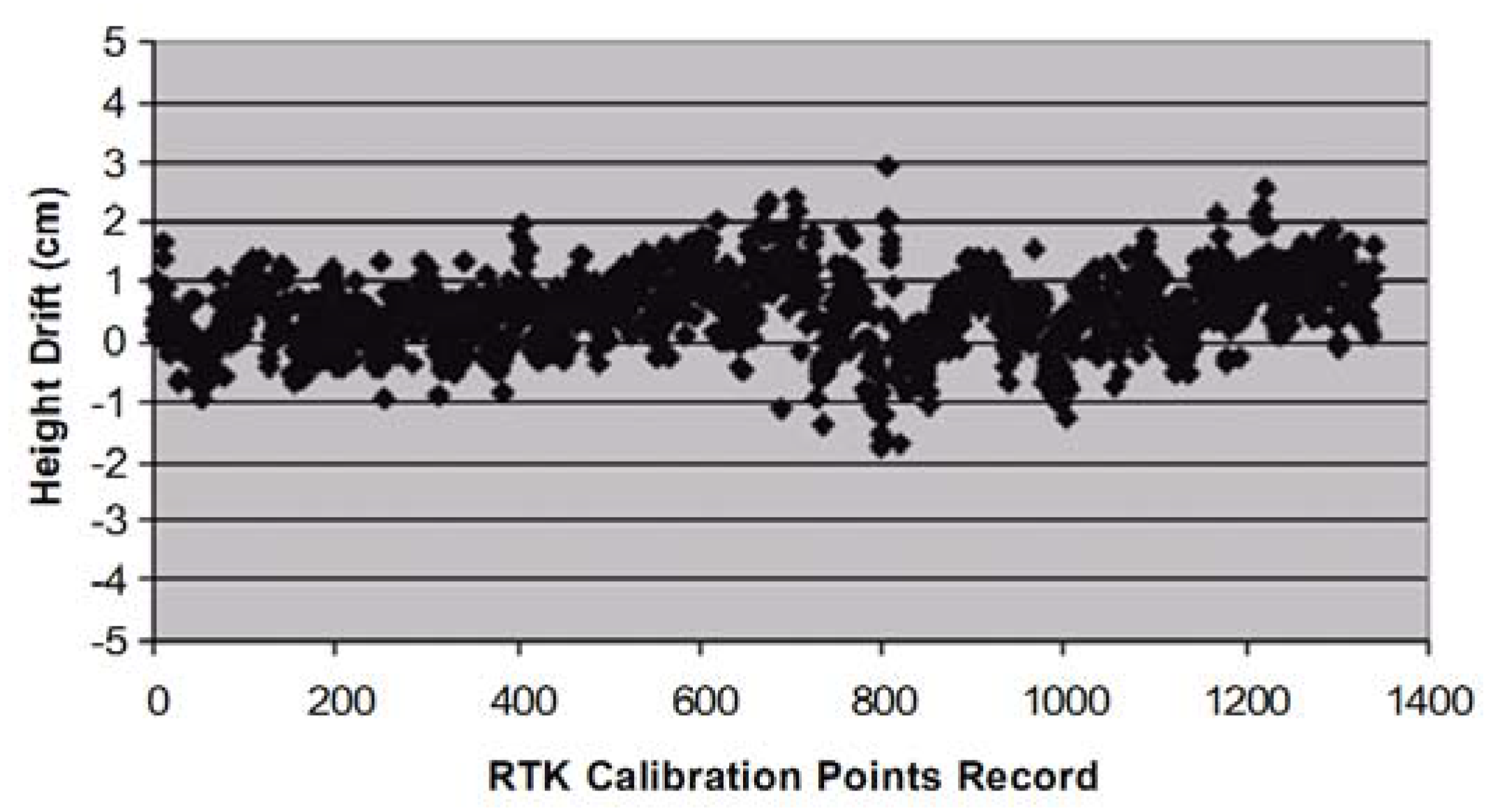
4.1. Testing of RTK-GPS Field Measurements

In order to determine the performance accuracy of the used RTK-GPS Topcon Hiper receiver, measurements over a short baseline connecting two known control stations was carried out. The accuracy of the receiver was determined by comparing the measured coordinates to the true coordinate values of known control survey station, over a baseline distance of 105.55 m. The rover receiver was set to collect coordinates continuously within an interval of 25 s. The total duration of the experimental measurement was approximately 2 h, with 1352 collected points. The results of the horizontal $(x,y)$ and vertical $(z)$ drifts are respectively presented as scatter plots in Figure 4 and Figure 5.

As depicted in Figure 4, the maximum value of horizontal position drift was 2.13 cm for easting and 0.97 cm for northing, with the trend of the horizontal position drift leaning to the negative (easting) values. The results for the vertical drift (Figure 5) values were lower than 2.00 cm. Overall, the GPS test results showed that the height drift was larger than the horizontal position drift, and confirms the fact that height accuracy of GPS should always be lower than the horizontal accuracy. Further, the receiver test root mean square errors (RMSE) summarized in

Table 2. Summary statistics for the RTK-GPS field evaluation.

Positional Drift	Minimum (cm)	Maximum (cm)	Average (cm)	Root Mean Square Error (RMSE) (cm)
Easting (x)	0.11	2.11	1.17	0.021
Northing (y)	0.10	0.84	0.48	0.026
Height (z)	0.15	2.92	1.21	0.017

indicates that the accuracy of the RTK-GPS is very high and fits to the specified Topcon Hiper instrument accuracy specification of (10 mm ± 1 ppm).

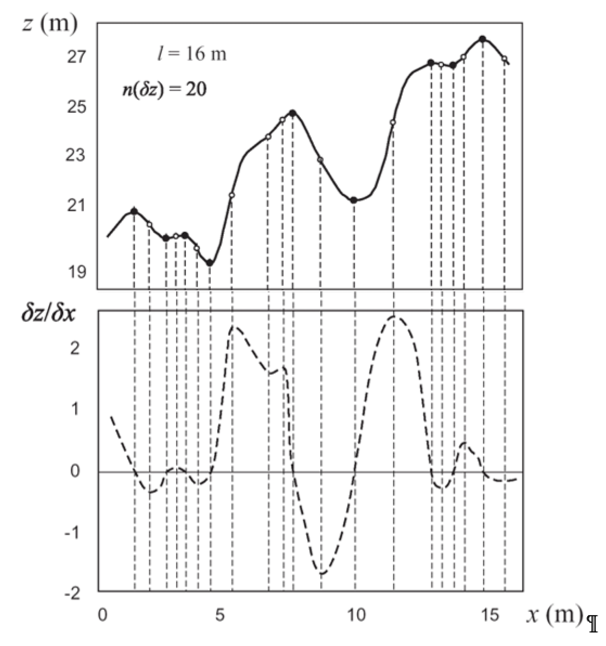
4.2. Selecting Suitable Grid-Size for DEM Generation Using RTK-GPS Surveys

In determining the optimal DEM grid size for terrain representation, the horizontal and vertical data resolutions are critical components [24]. In general, an increase in the detail in the DEM will also mean more accurate terrain parameters. This increase, however, depends on the general variability of the landscape. For example, a generally simple and smooth landscape might not need a fine resolution DEM. It would imply that the pixel size should be smaller than the average distance at which a distinct change in landform occurs.

The concept above can be illustrated by considering one-dimensional topography with specific number of inflection points, as depicted in Figure 6. An inflection point can be defined location at which the second derivative of a function (z) changes sign, i.e., location at which a function changes from being convex to concave and vice versa. Theoretically, the largest grid size $(g_{\max })$ should be at least the average spacing between the inflection points, and is represented by Equation (6).

$$g_{\max }\le \frac{l}{n\left(\delta z\right)}$$

(6)

where $l$ is the length of a transect and $n(\delta z)$ is the number of inflection points observed in the vertical (z) domain.

In Figure 6, there are 20 inflection points within the DEM, with an average spacing of 0.8 m between them. Hence, a grid size of at least 0.8 m is recommended. However, the selection of the most suitable grid size is not as simple as it seems. Because topography is a fractal feature, its roughness is practically immeasurable [24]. Hence, the number of inflection points also depends on the size of the argument $(\Delta z)$, which is somewhat similar to the concept of the grid size. This means that one can estimate the number of inflection points only after defining a certain grid size. With advancements in technology, this can be viewed to depend on the specific application and the limitations of the terrain data capture source, which with the availability of LiDAR point cloud data survey may not pose a limitation.

4.3. Uncertainty and Error Analysis for Optimal RTK-GPS Point Density

With the objective of illustrating how RTK-GPS can be used for storage capacity (volume) estimation for a proposed reservoir, this section presents an uncertainty and error analysis to define the appropriate point density. The point density variation is set so as to capture the required spatial data of the DTM representation.

To achieve this, the point density of the GPS survey was increased by varying the sampling grid sizes from regular square grids of 90 m to 0.1 m—through decimation by a factor of 3. The sampling scheme adopted in this study is depicted in Figure 7, whereby the grids are defined lengthwise (${}_l{g}_i$) and width-wise (${}_w{g}_i$). Such a scheme is expected to capture the critical points and features of the terrain such as pits, peaks, gully valleys ridges, hence taking into account the inflection points, as illustrated in Figure 6.

For the comparative analysis, both 90 m × 90 m and 30 m × 30 m ASTER Global DEM for the study area were downloaded. The decimation on the ASTERGDEM was carried out on the 30 m × 30 m DEM using nearest-neighbor resampling to correspond to the RTK-GPS point density. For the contour-based DEM generation, the 20 m contour interval lines were transformed from the topographic map into digital coordinate data using the sequential steps comprising of: scanning, georeferencing, digitizing and interpolation. The interpolation was based on natural neighbor method, because it is suitable for the interpolation and extrapolation of the digitized elevation contours.

Table 3. Size and distribution of DEM point densities for the study area.

Terrain Grid Size (gi)	Grid Points along the Length (gli)	Grid Points along the Width (gwi)	Maximum Number of Grids (ni) for a Grid (gi)	Maximum Point Density (di = Area/ni) (m2/point)
90 m × 90 m	13	3	39	6390
30 m × 30 m	38	10	380	874
10 m × 10 m	115	29	3335	100
3 m × 3 m	381	97	36,957	9
1 m × 1 m	1142	291	332,322	1
0.3 m × 0.3 m	3 807	970	3,692,970	0.09
0.1 m × 0.1 m	11,421	2908	33,212,268	0.01

presents a summary of the definition and distribution of point density for the study area, based on the grid sampling scheme in Figure 7. In practical implementation, point density must be high enough to capture the smallest terrain features, yet not too fine so as to grossly over-sample the surface, in which case there will be unnecessary data redundancy in certain areas [25]. This is the basis on which the RTK-GPS data collection for the reservoir area was implemented.

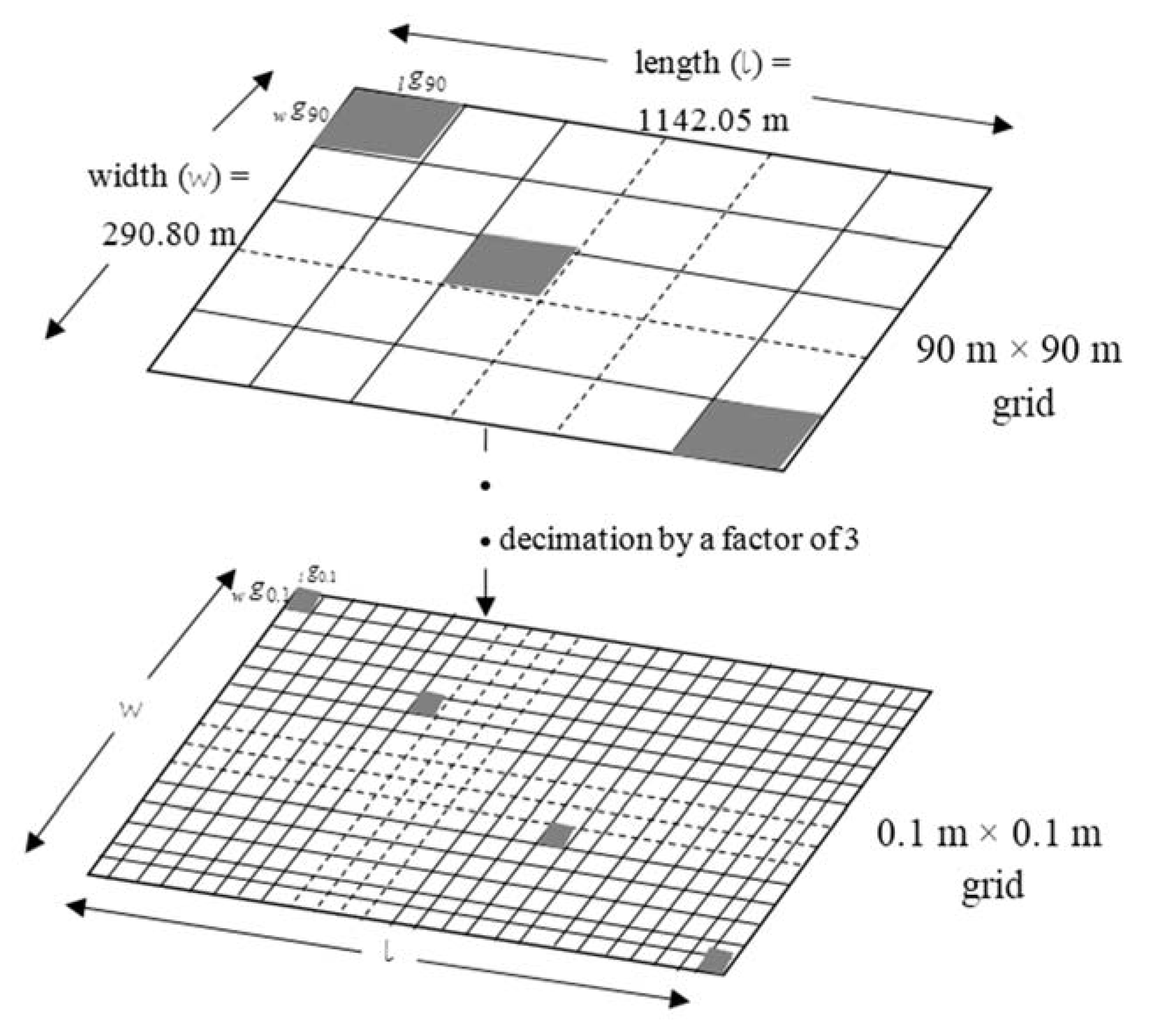
4.4. Procedure for Generation of the Proposed Reservoir Elevation Points

In this case study, the formal topological structure and variability of the terrain was taken into account, whereby the regular grid DEM data structure comprising of a matrix of elevations, sampled at regular intervals in both the $(x)$ and $(y)$ planes, according to the grid point density established in Table 3 were collected.

The initial survey of the points defining the proposed reservoir perimeter was carried out, and then merged to define the perimeter and the corresponding surface area. The results of the proposed reservoir defining perimeter points and area are respectively shown in Figure 8a,b.

Based on the pre-determined survey network of the reservoir perimeter, a dense network of gridded elevation points was observed and plotted, with illustrative results shown in Figure 8c, for the 30 m × 30 m grid size (corresponding to an average point density of 874 m²/point). In Figure 8c, section A-A represents a sample cross-section, while sections Y-Y and X-X are the representative long-sections. From the 3D RTK-GPS observed coordinates (Figure 8c), the reservoir terrain TIN was derived (Figure 8d).

TIN-based DEM is computationally efficient because of its coordinate random, but surface-specific characteristics. For accurate reservoir storage capacity/volumetric computations, the real surface depressions in the DEM are kept, i.e., the sinks and peaks are taken care of by defining the suitable transects. This is because generalized GPS sampling on large regular grids is inefficient for detailed and actual terrain features capture, especially for landscapes with varying slopes.

For the ASTER and contour DEM data sets, regularly-spaced elevation data were interpolated to grid DEMs by ordinary kriging based on the eight nearest neighbors. Semivariogram models were fitted to separation distances required to achieve eight neighboring elevation values. Cross validation, where each measured elevation point was removed individually and recomputed by the interpolation method, was used to evaluate interpolation errors. The semivariogram models and parameters were chosen to minimize these errors. For the study area, the Gaussian model was found to be optimal.

4.5. DEM Uncertainty and Error Analysis

Determination of errors in DEMs is often impossible because the true value for every geographic feature or phenomenon represented in a geographic data set is rarely determinable [26]. Uncertainty determination and error analysis can be used to describe the quality of a DEM especially at very high spatial resolutions [27,28].

Quantifying uncertainty and the resulting error in DEMs requires comparison of the original elevations with elevations in a DEM surface. To analyze the pattern of deviation between two sets of elevation data, conventional ways to yield frequency distribution of the statistical expressions of the accuracy, such as the dispersion measures, standard deviation, mean and root mean square error can be used [29]. In this study, RMSE (Equation (7)) was used as it measures the dispersion of the frequency distribution of deviations between the original elevation data and the DEM data.

$$RMS{E}_Z={\left[\frac{1}{n}{\displaystyle \sum _{i=1}^n{\left(Z_{di}-Z_{ri}\right)}^2}\right]}^{\frac{1}{2}}$$

(7)

where: $RMS{E}_Z$ is the root mean square error in the elevation $(Z)$; $Z_{di}$ is the i^th elevation value measured on the DEM surface; $Z_{ri}$ is the corresponding original elevation, and $n$ is the number of elevation points checked.

The larger the RMSE, the greater the discrepancy between the two data sets. When the true values (ground truth) are used as the reference data, the “uncertainty” becomes “error”. Accuracy is the reverse measurement of error. The accuracy of a DEM can be defined as the average vertical error of all potential points interpolated within the DEM grid [30]. In other words, it is the vertical root-mean-square accuracy of all points (infinitely many) interpolated in the DEM grid. Hence in this study the DEM uncertainty and error was analyzed, instead of the accuracy.

In assessing the accuracy of the results of the three DEM elevation sources, a suitable representative test area of 3600 m² with varying slopes, peaks and pits was chosen.

Table 4. Effects of DEM grid size and the accuracy measure in terms of root mean square errors (RMSE).

Grid Cell Size and DEM Data Source		$\mathit{R}\mathit{M}\mathit{S}{\mathit{E}}_{\mathit{Z}}$ (Meters)
0.1 m × 0.1 m	RTK-GPS	0.182
	ASTER	0.194
	Contour (planimetric)	0.198
1 m × 1 m	RTK-GPS	0.212
	ASTER	0.241
	Contour (planimetric)	0.202
3 m × 3 m	RTK-GPS	0.051
	ASTER	0.287
	Contour (planimetric)	0.293
10 m × 10 m	RTK-GPS	0.467
	ASTER	0.501
	Contour (planimetric)	0.525
30 m × 30 m	RTK-GPS	0.815
	ASTER 30 m Global DEM	0.866
	Contour (planimetric)	0.889
90 m × 90 m	RTK-GPS	0.922
	ASTER 90 m Global DEM	0.971
	Contour (planimetric)	0.986

shows the results of the comparative evaluation of grid resolutions at different elevation grid cell sizes as set out in Table 3. The true ground elevations were determined using conventional topographic surveying method, following the nature of the terrain. The results of the topographic surveying were aggregated and interpolated to suitable grid sizes as illustrated in Table 4.

The results in Table 4 show that the lower the spatial resolution of the interpolated DEM, the higher the RMSE. Notably, at 10 m and below there were significantly lower errors, as compared to larger and nearly equal errors at 30 m and 90 m sampling resolutions. RTK-GPS gave the least RMSE, followed by the contour-based DEM with ASTERGDEM giving the largest RMSE. The subsequent analyses in this study are thus based on RTK-GPS data, since it exhibited much higher accuracy for terrain parameter mapping. For further analysis, 3 m × 3 m grid size was chosen since it was considered not too fine to grossly over-sample the surface, and does not result into unnecessary data terrain capture redundancy.

Fundamentally, as the pixel size increases, a single DEM pixel value reflects more landscape area by averaging values within the pixel. For example, the 90 m resolution ASTERGDEM and contour DEM data have a single DEM elevation value for an area that is modeled by 9 elevation values in the ASTERGDEM and 30 m contour DEM and 81 values in the 10 m contour DEM. The effects of averaging elevation values for larger resolution models make them inherently less able to accurately model smaller variations found within the terrain. Thus, overall $RMS{E}_Z$ values increased with resolution as shown in Table 4. This implies that the horizontal resolution affects the vertical accuracy of the DEM data.

5. Estimation of Proposed Reservoir Surface Geometric Parameters from RTK-GPS Observations

This section presents the results of the estimation of the proposed reservoir’s surface area, slope geometry and the representative cross-sections and long-sections from the DEM.

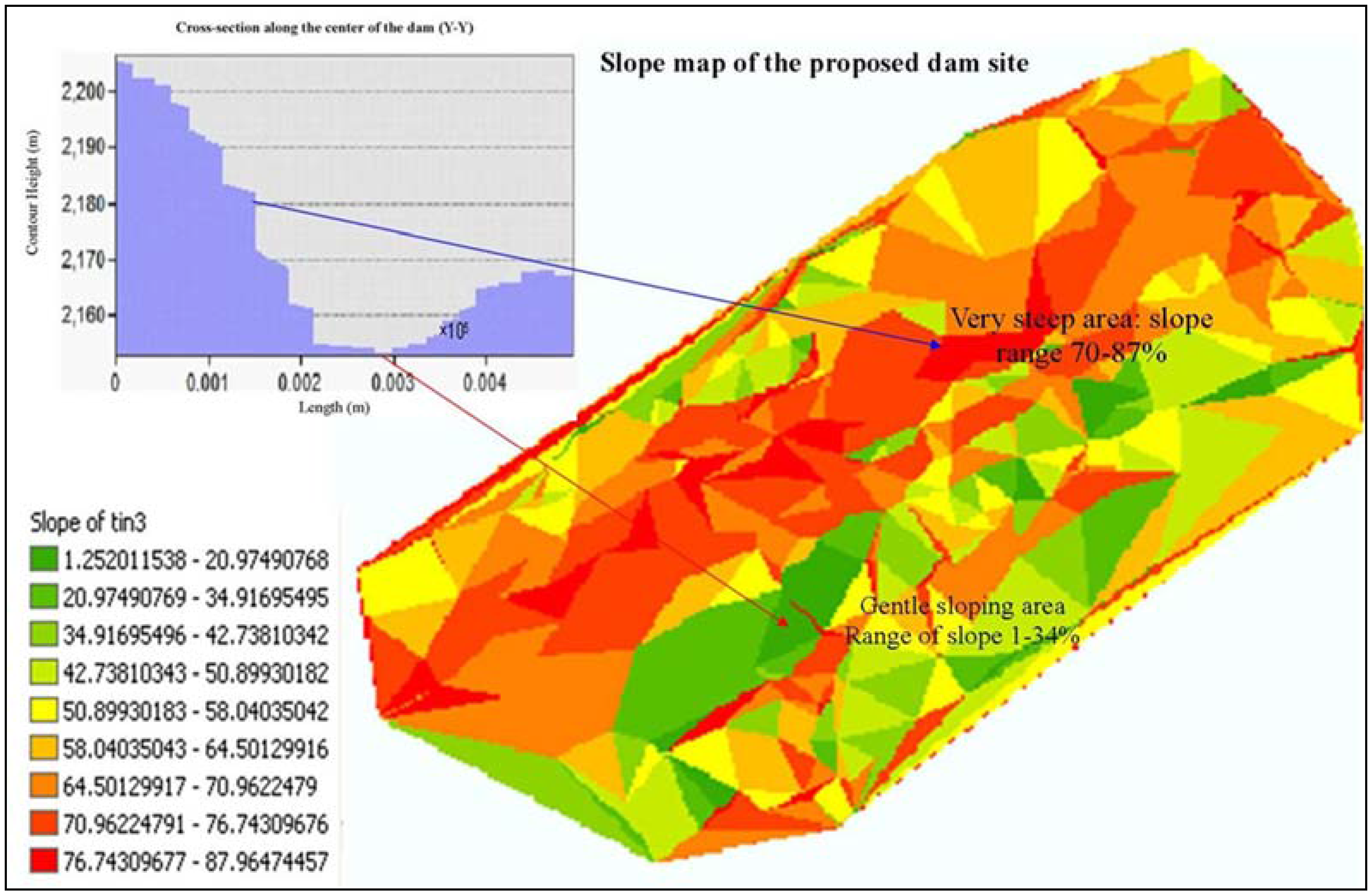
5.1. Reservoir Slope Derivation from DEM

In reservoir capacity estimation studies, very steep slopes may be unsuitable since they can be prone to erosion and landslides, as determined by the internal angles of friction of the soils. The following three methods as proposed by [31] were compared for slope calculation from the DEMs: (i) the Four Contiguous Right Triangles (FCRT) method; (ii) Maximum Downward Gradient (MDG); and (iii) Bicubic Spline First Derivatives (BSFD).

While the FCRT method takes into account the local elevation pattern and slope is calculated for a sub-pixel, the MDG method employs a comparison of the elevation of the central pixel in a 3 × 3 window with the neighboring eight pixels. The BSFD technique is based on the bicubic splines of the first derivative of the DEM, and tends to smooth out sharp slopes thereby having a tendency to present more gradient values ranging between 0° to around 45°. On the other hand, FCRT operator is complicated to process and the outputs are larger than the original DEM file, which is highly undesirable when dealing with vast data sets [31].

Since the MDG [32] operator gives a better approximation of terrain slope gradient as compared to FCRT and BSFD [31], it was adopted in this study for DEM slope computation. The results using the 3 m × 3 m RTK-GPS DEM (Figure 9) shows that while the upper sections of the reservoir are very steep, the lower ends tended to be fairly gentle. The average slope for the proposed reservoir varied between 40°–43° (i.e., slightly less than 50%), depicting fairly stable and suitable slope.

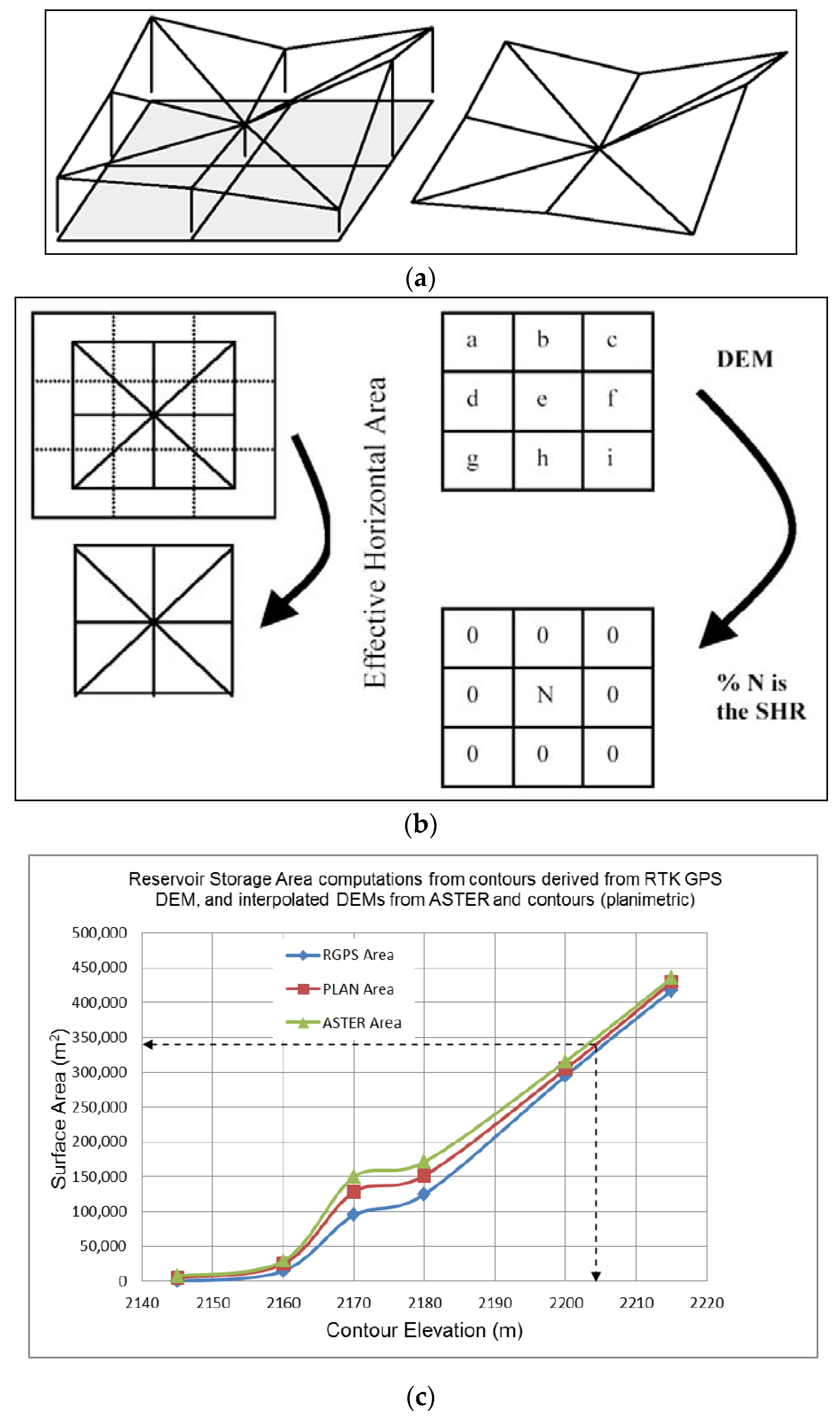
5.2. Reservoir Surface Area Computation Using Surface to Horizontal Area Ratio (SHAR) Based on Terrain Slope

An algorithm was developed for the surface area computation using a 3 × 3 moving window operator that triangulates the pixels in the optimal 3 m × 3 m GPS-derived DEM window into eight triangles, and then by extracting the elevation values from the nine pixels, the algorithm computes the surface area for each of the 8-triangular faces as demonstrated in Figure 10a. The equivalent horizontal area is then calculated for the corresponding region within the window (i.e., 4 times the pixel area), and then its ratio to the former is stored in the central pixel. This approach is advantageous as compared to conventional GIS approaches, where a linear relationship between vertices is assumed, while a bilinear representation is assumed within each DEM grid cell. The advantage of this approach is that slope surface area is calculated, and is a better indicator of the surface area than the conventional GIS-methods.

As depicted in Figure 10b, the program operates on a 3 × 3 window basis and calculates the surface area of the window by triangulation. The Surface to Horizontal Area Ratio $\left(SHAR\right)$, which is equivalent to the Surface to Horizontal Ratio $\left(SHR\right)$ (Equation (8)) is stored as a percentage so as to minimize errors in float to integer conversions [33].

$$SHAR=\left\{\left(SA\right)/\left(HA\right)\right\}\times 100$$

(8)

where $SA$ is the summation of surface area for each 8-triangles (Figure 10b), and $HA$ is 4-times the pixel resolution area.

The surface area for each pixel $S{A}_P$ is then calculated from the $SHAR$ according to Equation (9).

$$S{A}_P=\left\{SHAR\times A_P\right\}/100$$

(9)

where $A_P$ is the area of each pixel in the generated raster DEM.

As in Equation (8), the value of $SHAR$ can never be less than one since the surface area is greater than or equal to the horizontal area. Moreover the upper limit of this value though theoretically is infinity, but practically it is finite since a slope value of 90° is not practically derivable from a DEM. $SHAR$, being the focal function equivalent of the areal parameter (which is a global function), is suitable for further local, focal, zonal or global comparative overlaying operations.

Using the $SHAR$ based area computations, the surface area of the proposed reservoir was determined to be 332,109 m². The RTK-GPS DEM-surface area was compared with the ASTER and the planimetric (contour-based) surface areas with results shown in Figure 10c. The optimal elevation corresponding to the $SHAR$ determined area is about 2205 m. The results show that ASTER and planimetric data marginally overestimated the reservoir surface area, as compared to the GPS data source, especially between elevations 2155 m–2185 m (Figure 10c). At lower and higher elevations, the results of the three data sets were comparable. This observation corresponds to the RMSE results in Table 4.

A quantitative comparative fit of the area results showed that the planimetric (PLAN_AREA) and RTK-GPS (R_GPS_AREA) surface areas are related according to the deterministic relationship: $PLA{N}_{AREA}=0.915\times RGP{S}_{AREA}$; while the ASTER (ASTER_AREA) and RTK-GPS areas area related by: $ASTE{R}_{AREA}=0.922\times RGP{S}_{AREA}$. The closeness of the constant factors between the two area relationships validates the $SHAR$ computational results.

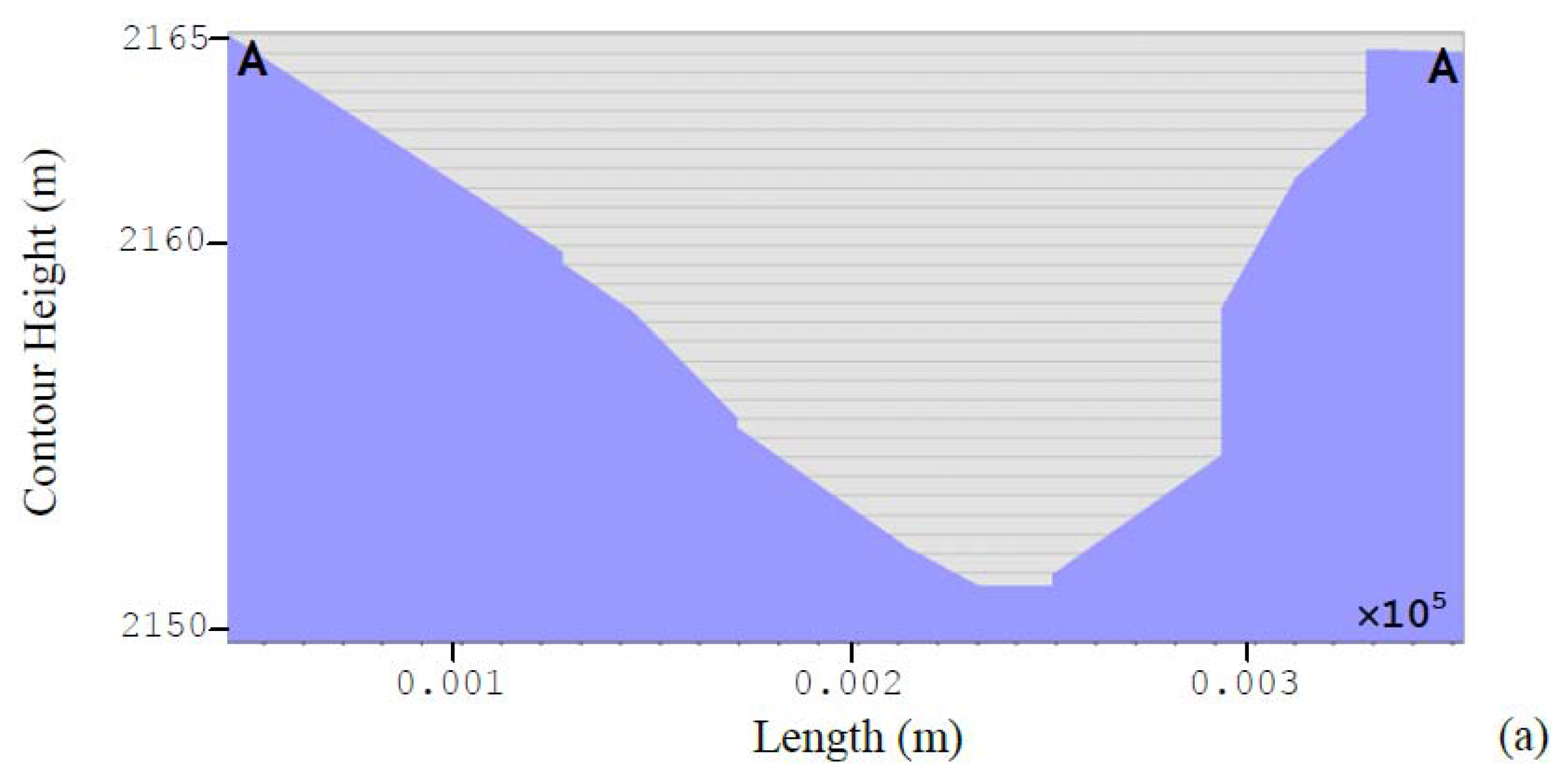
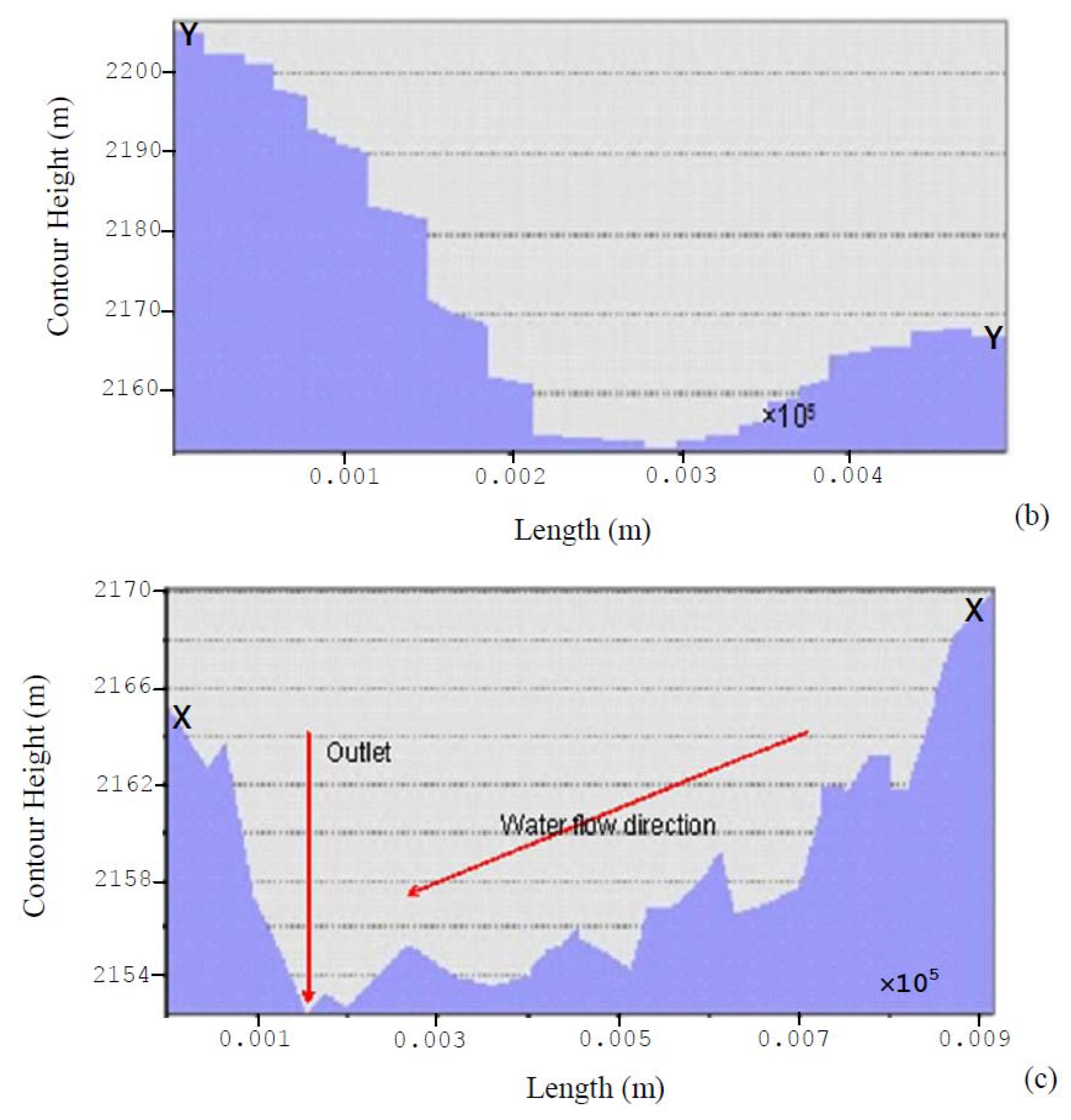
5.3. Reservoir Cross-Sections and Long-Sections

Characterization of reservoir cross-sectional information is significant in hydrologic studies for dam design. Cross-sectional geometric elements are useful in the determination of the reservoir formation levels, computations of the volumes of earthworks and in the determination of the potential reservoir storage capacity. From the 3 m × 3 m GPS DEM, representative cross-sections and long-sections were derived. These sections depict the transverse and longitudinal nature of the existing reservoir topographical surface, and the vertical alignment of the reservoir surface segments. The derived cross-sections (A-A) and long-sections (Y-Y and X-X) depicted in Figure 8c are represented in Figure 11, for the proposed reservoir.

As in Equation (1), the Y-Y and X-X sections approximately represents the length of the dam and the dam reservoir throwback or fetch, from which the surface area and capacity can be estimated using the direct methods as introduced in Section 2 of this study.

6. Comparative Evaluation of Reservoir Storage Curve Determination

This section presents the results of the reservoir storage volumetric computations using RTK-GPS-based DEM in comparison with the ASTER Global DEM and planimetric interpolated contour based DEM. Derivation of storage curve elements as defined by the volume-depth and volume-area power curve relationships are also presented as essential reservoir planning, design and monitoring parameters.

6.1. On the Influence of Sampling Point Density on Reservoir Storage Volumetric Computations

Storage volumes computed from the three DEM sources were compared in order to understand the significance and effects of the DEM data source and the spatial density sample spacing (grid cell size) on reservoir terrain attribute characterizations. Results of the comparative volumetric computations are presented in Figure 12. The differences in data sources were measured relative to RTK-GPS—as the most accurate data source, from the RMSE results presented in Table 4. Figure 12 presents the results for the volume computations based on the variations of the grid sizes for the elevations derived and interpolated from the three elevation data sources. The area used in the computation is from the SHAR approach. The empirical analysis of the relationship between the volume and the point density is then used to derive their mathematical relationship.

Storage volumetric computation results in Figure 12 shows that for the three datasets, the maximum storage volumes were comparable, with a maximum storage volume of 4.35 × 10⁵ m³ being observed from the contour-based planimetric method, and a minimum storage volume of 3.96 × 10⁵ m³ being determined from RTK-GPS based DEM. The differences in the results could be attribute to the fact that the interpolation process in creating the DEMs resulted in generally higher volumes from the planimetric and ASTER DEMs.

The reservoir capacity results of the lower grid cells (0.1 m–3 m) were generally closer, as was also observed between 30 m and 90 m. In overall, ASTER and contour-based volumes were consistently higher than the RTK-GPS-based volumetric computations. These results depict the fact that apart from the point density (which is directly proportional to the grid cell size), the intervals and transects between the grids also impacts on the storage-stage curve.

The results in Figure 12 and Table 3 illustrate the fact that the capacity of a reservoir is a function of the DEM point density $(d_i)$ according to Equation (10). This empirical relationship illustrates the fact that reservoir volume and the certainty of determination, as derived from GPS point data, is dependent on the point density variations. The significance of this relationship is that it enables the determination of the “saturation” point density size or grid cell size, below which the computed volume will be statistically unchanged.

$$V_e=c\times d_i^{\rho }$$

(10)

where: $V_e$ is the difference between the estimated and true volume of the reservoir; $c$ is a regression constant of $V$ on $d_i$; $d_i$ is the point density (m²/point) corresponding to the grid cell size of $i$ × $i$, and $\rho$ is an exponent of the power relationship for $V-d_i$.

The factors $k$ and $\rho$ are site specific variables that depend on the optimal grid cell size $i$ (or $g$). Further experimentation needs to be carried out on other sites of varied terrain shapes and characteristics, slope (peaks and pits) and area extent in order to generalize the relationship proposed in Equation (10).

6.2. Reservoir Volume-Depth Estimation

Using the predetermined surface areas and the corresponding reservoir depths D, the surface area-depth $(A-D)$ relationship was derived and used to calculate the reservoir capacity $(V)$, according to [34] Takeuchi (1997). The storage capacity of the reservoir was computed with the results in Figure 13. In Figure 13, the volume is computed directly from DEM by multiplying the proposed water level surface difference raster with the grid cell area. The results in Figure 13 (main figure and the inset) represent the same data, with the main line graph showing the depth increasing from 2150 m to 2210 m and the inset figure representing the critical volume-depth relationship from 2150 m to 2170 m. In practice, the main figure gives the overall volume-depth relationship which can be used during the designs stages and for post-design reservoir monitoring and or expansions. The inset figure is for the visualization, planning and design decisions in the specified elevation regions of the V-D curve.

The results in Figure 13 depict the expected relationship that the volume contained within a reservoir increases with an increase in depth. In this case study, the depths can be segmented into two zones of 20-m each: i.e., 2150 m–2170 m and 2170 m–2190 m, with the former being the optimal depth. Further, the obtained reservoir $V-D$ relationship is significant in evaluating: (i) the length of the dry period over which a given level of supply can be maintained; (ii) the water level during supply that can be maintained during a given dry period; and (iii) in assessing the relative significance of the evaporation losses as compared to the water consumption.

From the results in Figure 10, Figure 12 and Figure 13, the RTK-GPS results are consistently in the lower bound estimation of the storage volume as compared to the ASTER and planimetric-contour results. By evaluating the different data sources as in this study, the optimal storage capacity in terms of the possible minimum and maximum can be inferred. In practice, it is better to slightly underestimate than to overestimate the reservoir capacity so as to achieve an optimal design in the end. At the design stage, the reservoir is usually slightly overdesigned to take care of excess water availability and to compensate for the operational storage; equalizing storage; standby storage; fire suppression storage, and dead storage.

6.3. Storage Capacity-Area Power Relationship

From the surface area and depth variations, changes in the water storage volumes $(\Delta V)$ can indirectly be regressed from changes in the surface area. According to [34] Takeuchi (1997), the relationships between $D,A$ and $V$ can be expressed according to the following Equations (11)–(13).

$$A=\alpha \times D^{\beta }$$

(11)

$$V=\gamma \times D^{\eta }$$

(12)

$$V=a\times A^b$$

(13)

where: $\alpha ,\gamma \text{ and }a$ are constants, and $\beta ,\eta \text{ and }b$ are the respective exponents of the power relationships for the A-D, V-D and V-A relationship curves.

The results for the analysis of the storage capacity variations with the reservoir surface area and multiresolution DEMs are presented in Figure 14a. The results indicate that the 3 m grid size is the balance V-A line, whereby DEM resolution does not grossly overestimate and underestimate the reservoir storage capacity as the surface area increases [35]. While the accuracy of DEMs depends on their grid sizes or resolutions, the acquisition technologies, sources of the original data and interpolation methods [18], and that higher resolution DEMs provide more accurate representations of topographic features, [36] found out that much higher improvements in DEM resolutions did not necessarily result into improved watershed hydrologic modeling. This implies, as observed in this study, that grid resolutions of less than 1 m may not only be practically difficult to acquire using terrestrial surveys, but may also not result into better accuracy.

Adopting the [34] V-A power curve relationship in Equation (13), this study determined that for the proposed reservoir, the volume-area storage power curve was defined by the deterministic exponential function: $V=0.09\times A^{1.435}$ for the RTK-GPS model. The determination coefficient for this relationship was highly correlated at $96.8\%$ confidence. The $V-A$ relationship result in Figure 14b indicates that the disparities between the determinants marginally increase with the increase in surface area.

In practice, for effective reservoir utility, the storage volume of the reservoir should not exceed 10% of the annual catchment contribution. With an estimated annual catchment contribution of 3.8 × 10⁶ m³, the results in Figure 14b shows that an optimal capacity of 4.0 × 10⁵ m³ is possible from the 3 m grid size (Figure 12). This is within the acceptable value, i.e., 9.5%, of the catchment rainfall contribution.

The determined reservoir volume and surface area can also be used to derive the maximum relative storage capacity index $(S_R=V/A_r)$, which is a measure of the runoff height that can be stored in the reservoir relative to the total area of the reservoir $(A_r)$. For the case study, the $S_r$ index was calculated as 1.2 m. This is greater than the reservoir volume to catchment surface area ratio, meaning there are lower chances of flooding or overflow at optimal or peak performance.

6.4. Reservoir 3D Storage Capacity Simulation

Once the optimal storage area and volume have been determined, reservoir 3D representation is useful in the capacity simulation and visualization of the related hydrologic and spatial attribute data. Simulated reservoir water levels and capacity supports in spatial and attributes information inquiry, in the real-time monitoring and management, and can also be used to monitor and simulate flood submergence and drought conditions.

The results of the simulated waters for the proposed reservoir, using the RTK-GPS survey results is presented in Figure 15. The 3D representation further shows that the right side of the reservoir will have to be elevated to contain the desired optimal capacity. Inset in Figure 15, is the cross-sectional area relative to the embankments at contour elevation of 2165 m. An additional elevation of 5 m will realize the proposed optimal maximum depth of 2170 m, hence reaching the optimal reservoir capacity of 4.0 × 10⁵ m³.

6.5. Validation of the Proposed Model with in Situ Data

The reliability of model output depends on how well the model structure is defined and how well the model is parameterized. Estimation of model parameters is normally sensitive and challenging due to uncertainties associated with the determination of parameter values that cannot be obtained straight from the field. By comparing in situ storage reference data from the existing storage curve with the simulation results, the reliability of the proposed model was assessed.

Since the storage volume in reservoirs at the beginning and end of the rainy seasons is a key variable of water availability in semi-arid areas, such as the case study area, the percentage differences between the simulated and observed in situ storage volumes in the corresponding months of May, June, July, August ($d_{V,t}$) for the existing Kesses reservoir I (Figure 2) were used to determine the deviation reliability of the model. The four months were chosen since they represent the minimum to maximum storage volumes and depths in the reservoir.

In order to evaluate the model performance in simulating the temporal behavior of storage volumes in the Kesses reservoir I, the Nash-Sutcliffe coefficient of efficiency ($e_V$) [37], based on the monthly observed and simulated reservoir storage volumes ($V_{obs,t},V_{sim,t}$) was computed as expressed in Equation (14), in order to assess the predictive power of model for reservoir storage volume determination. For model validation, observed average time series were compared to the simulated series of the mean reservoir.

$$e_V=1-\frac{{\displaystyle \sum _t{\left(V_{obs,t}-V_{sim,t}\right)}^2}}{{\displaystyle \sum _t{\left(V_{obs,t}-\overline{V_{obs}}\right)}^2}}$$

(14)

where: $V_{obs,t}$ is the observed volume and $V_{sim,t}$ is the simulated volume from RTK-GPS, both at time $t$, and $\overline{V_{obs}}$ is the mean observed monthly storage volume.

The validation results showed that in terms of water storage volumes, the model deviations from the observations at the beginning and end of the rainy seasons ($d_V$) were less than +10% (Figure 16a). The 12-month variations in the model performance efficiency ($e_V$) varied between +0.9 to +0.4, with an average model efficiency of +0.7 as shown in Figure 16b. The validation results show that there is no major tendency of systematic over- and or underestimation, meaning that the model reasonably estimated the average water storage volumes.

7. Results and Discussion

In this section, considerations of the potential reservoir capacity and geometrical elements are outlined and analyzed based on the results of the current study.

(a)

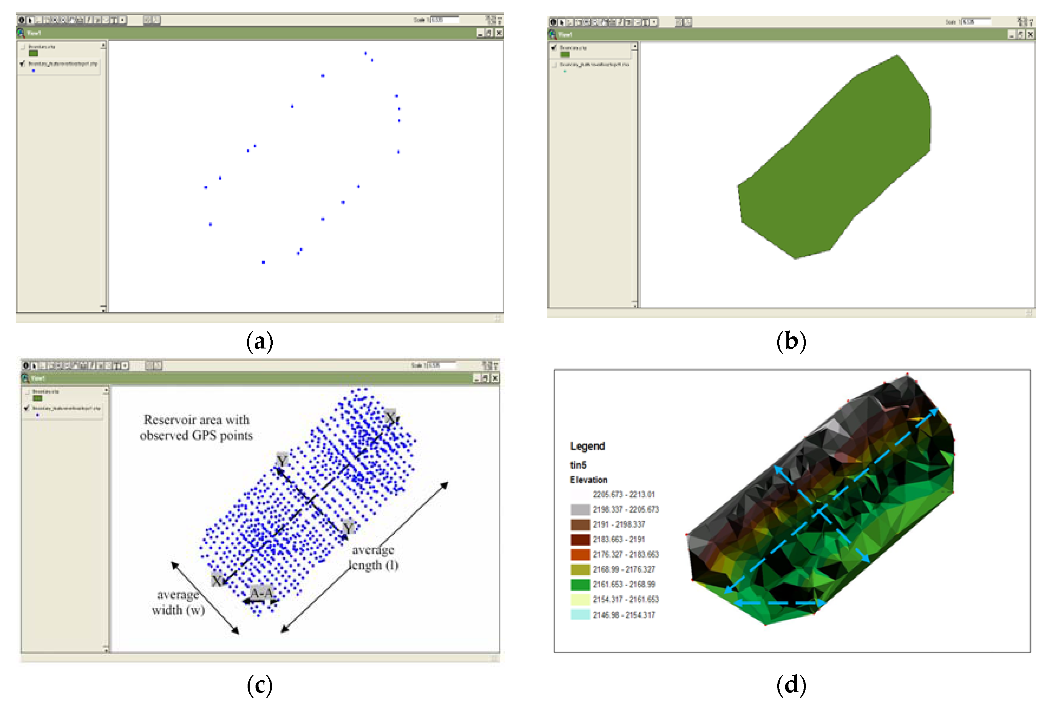
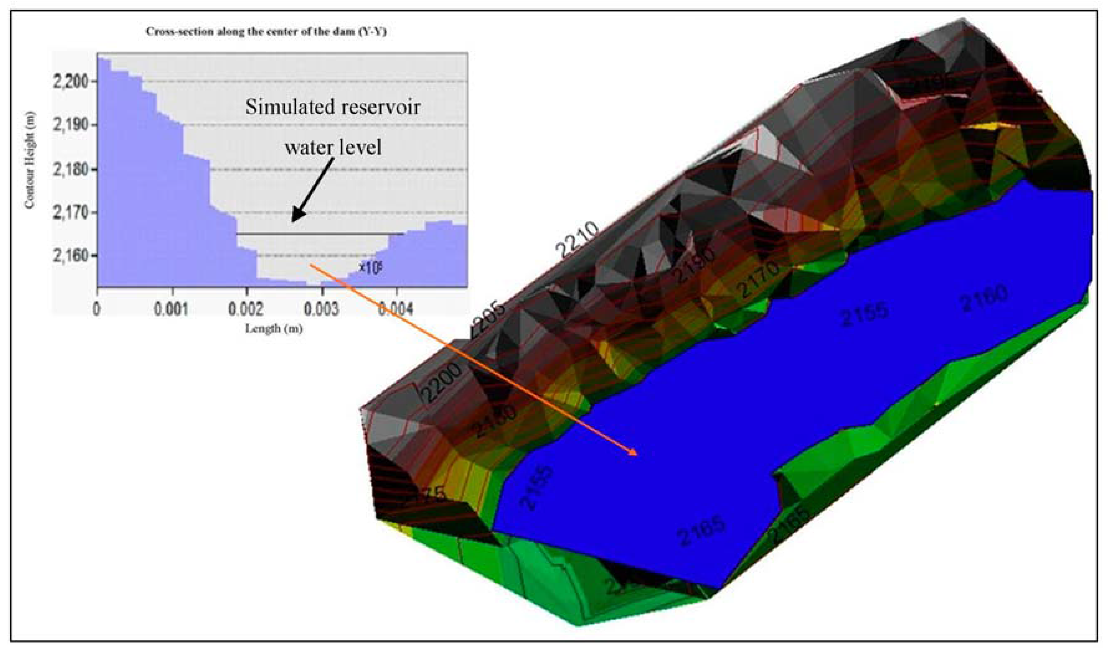
Reservoir topography and dam site selection: The slope results show that the proposed reservoir site has a uniform steep-slope, which is suitable in supporting the reservoir embankments. Under ideal conditions, the dam should be located in the narrow sections of the river, just downstream of relatively wide stretch, and with minimal slope angles. This condition requires narrow valley stretches with relatively steep sides up to the required water level, above which one of the embankments flattens considerably. With this consideration, the cross-section along the reservoir axis A-A (Figure 11a), and as depicted in the inset in Figure 15, was suggested as the suitable dam site for the proposed reservoir.

Further, the inclinations of the surfaces from the terrain aspect, shows that there are three major slope directions in this area. These directions form a V-shaped configuration which represents the suitability of the proposed site as being a basin, enabling the retention of water over longer temporal intervals and provides the catchment outlet in a narrow valley that is suitable for locating the dam axis.

(b)

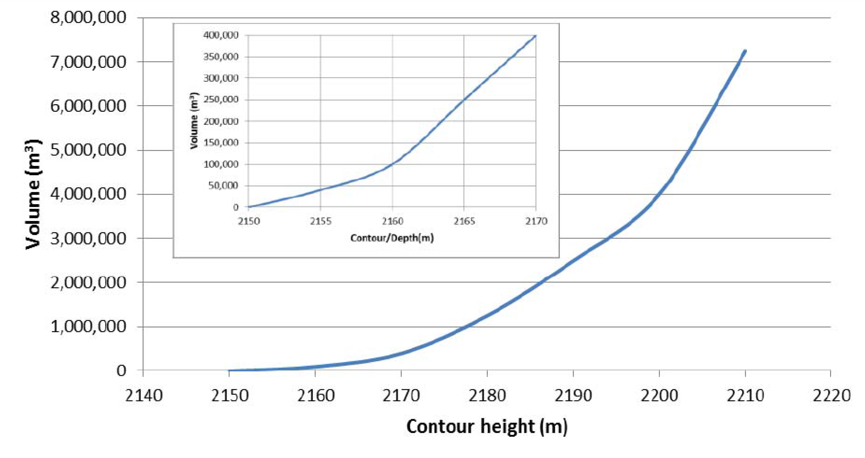
Size of the catchment area and area of proposed reservoir: For sustainable water supply, it is required that the catchment or watershed area should be large enough to ensure replenishment of the reservoir even in moderately dry seasons. Considering the entire catchment area, the reservoir will receive most of its waters from the existing Kesses reservoir I.

The study results show that the surface areas increase with increase in contour height. This is expected to be so because the land does not slant vertically, but is gradually inclined with a mean slope angle of 41.5°. Based on the results, if the maximum contour depth difference $(\Delta D)$ is set to be 20 m, then the corresponding water surface area and capacity can be monitored from the resulting V-A and V-D plots.

(c)

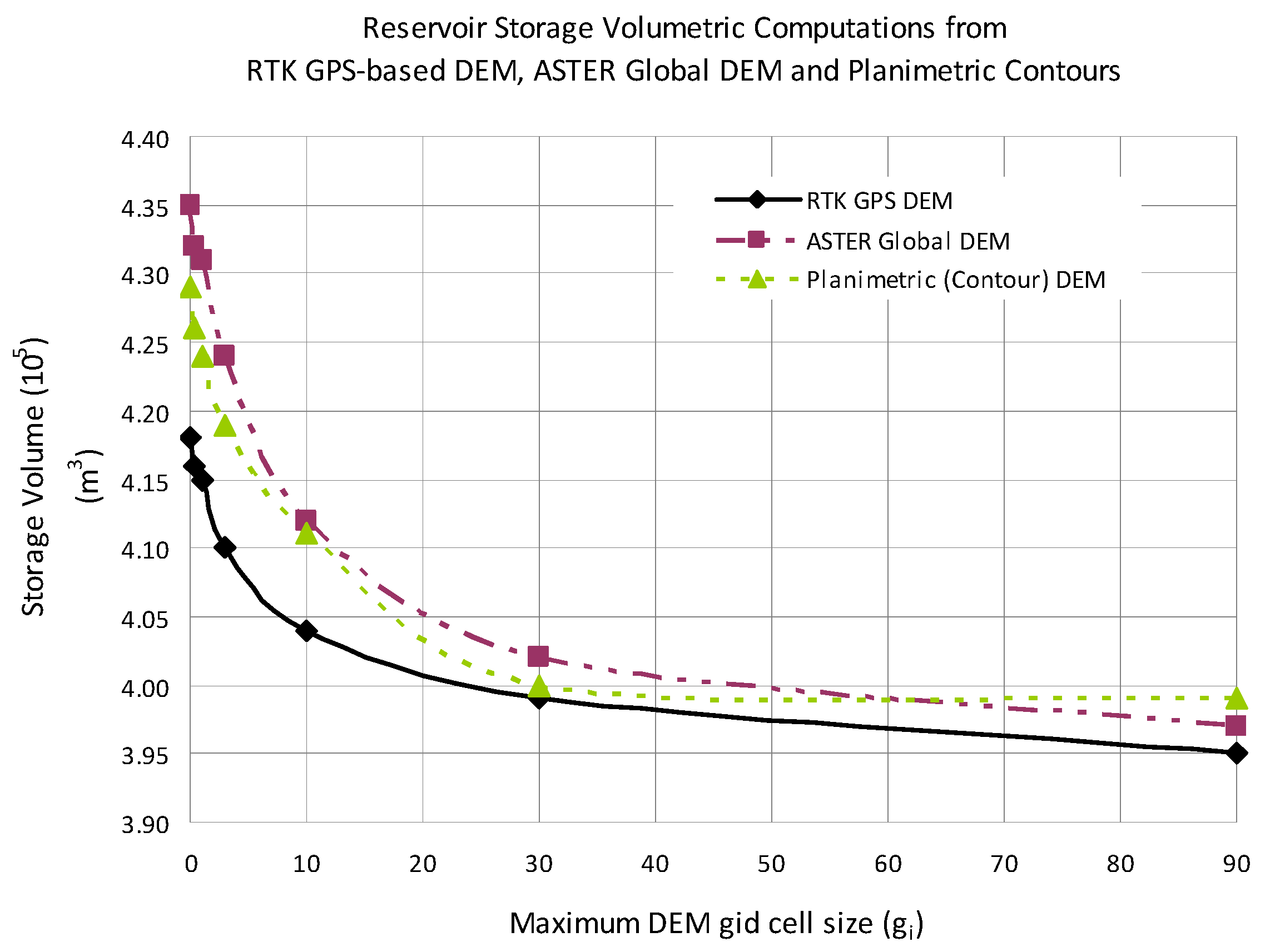
Quality of DEM generation: The results and discussions in (a) and (b) above are based on the RTK-GPS generated DEM. These results shows that the quality of a DEM is dependent on a number of interrelated factors, such as the methods of data acquisition, the nature of the input data, and the methods employed in generating the DEMs [38]. Notably, the higher values of the storage volumes determined from the ASTER DEM and planimetric contour interpolation, as compared to the RTK-GPS observations could be attributed to the fact that the interpolation procedures for DEM generation in the former data sets are generally not accurate.

Based on the results from this study, the DEM data spatial resolution and point distribution is the most critical factor as depicted in Figure 17. Figure 17 illustrates the significances of different spatial resolutions on detail representation (Figure 17a–d), and the corresponding 3D terrain geometric computations, e.g., slope (Figure 17e). In Figure 17f, the 10 m DEM (i) depict slopes from 10° to areas of greater than 50°. The 30 m DEM (ii) represents highest slope, in this example, greater than 30°, while the 90 m DEM (iii) shows only slopes of no more than 20°. These disparities in slope calculations clearly imply that the spatial resolution of a DEM is critical in capturing the terrain derivatives. The observation in Figure 17 confirms the proposed mathematical correlation between the storage volume and the smallest size of pixel representing the DEM terrain as expressed in the proposed model in Equation (10).

(d)

Correlation between DEM uncertainty, accuracy and GPS point density: Uncertainty and error analysis using root-mean-square-error showed that the inherent errors in DEM were mainly due to the data acquisition process, source and the interpolation process. The results showed that high uncertainty and therefore DEM error tended to concentrate in rugged terrain areas, especially when the densities were high (corresponding to high grid cell sizes). On the variability of the topography and DEM resolution, it is noted that even in naturally varying topography, it may not be accurate to generalize that the lower the grid size, the more accurate the results will be. Rather, this should be dependent on a specific scene and also on the morphologic features of interest.

(e)

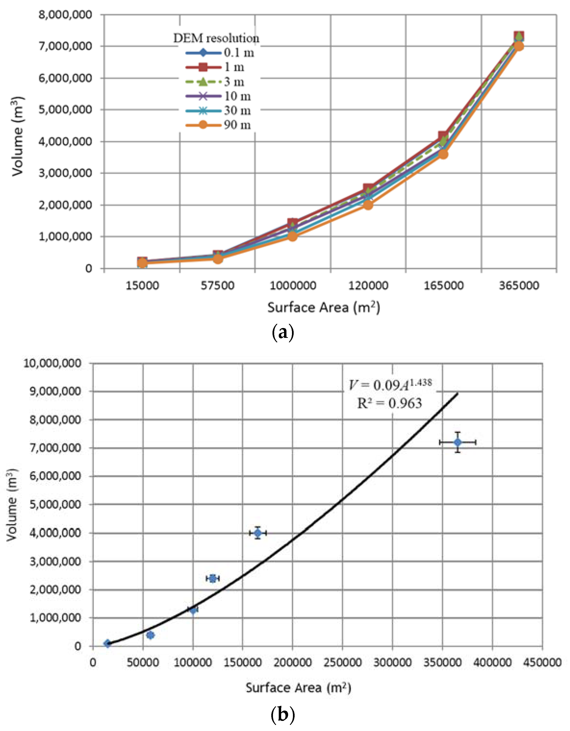
On the relationship between elevation and GPS point density for optimal DEM determination: From the results in Figure 10, it is observed that the surface area computation results for the three DEM data sources do not deviate so much from each other, with RTK-GPS results consistently giving a lower bound estimate of the reservoir surface area. The same consistency is observed in Figure 12, with saturation in the reservoir volume being observed at 30 m × 30 m grid resolution. In Figure 12, a higher storage capacity is observed between 0.1 m and 3 m. The results in Table 4 confirm that 0.1 m to 1 m grid sizes may overestimate the proposed reservoir storage capacity and this is also observed the in the RMSE results in Table 2. The results in Figure 10 imply that for more accurate surface area determination, the higher grid density is more suitable in nearly smooth and natural terrain. This is because DEM grid sizes and the corresponding reservoir surface areas tend to reach a peak beyond which further potential reservoir storage information may not be feasible. The implication is that there is a corresponding linear relationship between the surface area-elevation (Figure 10) and the volume-GPS DEM point density (Figure 12), which are important in the derivation of the V-D power curve as systematically derived in Section 6.1 above.

An analysis should be extended into the impacts of different data collection patterns, e.g., random versus systematic; significant points versus terrain contouring. This is because the accuracy of the spatial interpolation of elevations is subject to input data points density and distribution, which in turn determines the estimated volumes.

8. Summary and Conclusions

This study explored the potential and efficacy of deriving high-resolution DEM from RTK-GPS for reliable reservoir storage capacity estimation and geometrical characterization for a simple terrain. The study proposed an approach for the estimation of the reservoir storage curve and the geometric properties by using a suitable multi-grid analysis method. This approach resulted into a near-continuous surface representation from the discrete RTK-GPS observations. The approach is considered advantageous to GIS methods, where a linear relationship between vertices is assumed, while a bilinear representation is assumed within each DEM cell.

The results for the proposed Kesses reservoir II showed that RTK-GPS approach can be used to accurately determine and predict the desired reservoir capacity-area power curve and the related geometric surface parameters by setting up suitable sampling techniques, based on GPS point density and observational transects.

The findings from the study further shows that the power relationships between the reservoir surface area and the simulated storage capacity was defined by the deterministic function $V=0.09\times A^{1.435}$. In terms of accuracy measurements, confidence testing at 95% limit using Pearson correlation analysis indicated that the variances of the reservoir surface areas as determined from the RTK-GPS, ASTER and planimetric DEMs were slightly different, i.e., $\left(p<0.20\right)$. These depicted that the critical issue of estimating the storage capacity of a reservoir is not only on the accuracy of measurement, but on the ground data sampling and interpolation strategies that influences the ability to cover area with optimally representative sample points. The model validation against observed reservoir storage volume shows that the proposed approach is reasonable in assessing the surface water availability, and can accurately be used to infer the reservoir stage-storage relationship (SSR).

While the results of this study are site specific, they can methodologically be replicated to: (i) infer the A-D and V-D correlations; (ii) approximate the unknown A-D and V-D relations for a proposed reservoir; and (iii) serve as a model for the simulation, design and future monitoring of the reservoir. The proposed methodology can be used as an alternative to the conventional methods of topographic data acquisition and processing for reservoir designs, and offers the advantage for reservoir monitoring. While the current results are for simple terrain, the same DEM acquisition method and methodological approach can be applied for any type of terrain where there is need for reservoir planning, design and construction. For an existing reservoir with design data, the method can be used to compare and automate the reservoir monitoring and redesign. Thus being an advantageous technique to the conventional reservoir or lake monitoring and reservoir re-design.

In recommendation, further studies should be carried out evaluate the quality and efficiency factors between RTK-GPS surveys and InSAR and LiDAR data in reservoir DTM surface representations and analyses. Also the proposed volume-point density relationship should be further investigated on for generalization.

References

1. Guo, S.L.; Zhang, H.G.; Chen, H.; Peng, D.Z.; Liu, P.; Pang, B. A reservoir flood forecasting and control system for China. Hydrol. Sci. J. 2004, 49, 959–972. [Google Scholar] [CrossRef]
2. Keller, A.A.; Sakthivadivel, R.; Seckler, D. Water Scarcity and the Role of Storage in Development; IWMI Research Report 039; International Water Management Institute: Colombo, Sri Lanka, 2000. [Google Scholar]
3. Van der Zaag, P.; Gupta, J. Scale issues in the governance of water storage projects. Water Resour. Res. 2008, 44. [Google Scholar] [CrossRef]
4. Hayashi, M.; van der Kamp, G. Simple equations to represent the volume–area–depth relations of shallow wetlands in small topographic depressions. J. Hydrol. 2000, 237, 74–85. [Google Scholar] [CrossRef]
5. Mongus, D.; Zalik, B. Parameter-free ground filtering of LiDAR data for automatic DTM generation. ISPRS J. Photogramm. Remote Sens. 2012, 67, 1–12. [Google Scholar] [CrossRef]
6. Wang, L.; Yu, J. Modeling detention basins measured from high resolution LiDAR data. Hydrol. Process. 2012, 26, 2973–2984. [Google Scholar] [CrossRef]
7. Magome, J.; Ishidaira, H.; Takeuchi, K. Method for satellite monitoring of water storage in reservoirs for efficient regional water management. In Water Resources System—Hydrological Risk, Management and Development; Bloschl, G., Franks, S., Kumagai, M., Musiake, K., Rosbjerg, D., Eds.; IAHS Publ.: Sapporo, Japan, 2003; pp. 303–310. [Google Scholar]
8. Nico, G.; Leva, D.; Fortuny, J.; Antonello, G.; Tarchi, D. Generating digital terrain models by a ground-based synthetic aperture radar interferometer. IEEE Trans. Geosci. Remote Sens. 2005, 43, 45–49. [Google Scholar] [CrossRef]
9. Ferrari, R.L. Lake Arrowhead 2008 Reservoir Survey; Technical Report No. SRH-2009-9; U.S. Department of the Interior: Washington, DC, USA, 2009.
10. Wilson, G.L.; Richards, J.M. Procedural Documentation and Accuracy Assessment of Bathymetric Maps and Area/Capacity Tables for Small Reservoirs; U.S. Geological Survey Scientific Investigations Report 2006-5208; USGS: Reston, VA, USA, 2006.
11. Magome, J.; Takeuchi, K.; Ishidaira, H. Estimating water storage in reservoirs by satellite observations and digital elevation model: A case study of the Yagisawa Reservoir. J. Hydrosci. Hydraul. Eng. 2002, 20, 49–57. [Google Scholar]
12. Peng, D.; Guo, S.; Liu, P.; Liu, T. Reservoir storage curve estimation based on remote sensing data. J. Hydrol. Eng. 2006, 11, 165–172. [Google Scholar] [CrossRef]
13. Stephens, T. Handbook on Small Earth Dams and Weirs; Cranfield Press: Bedford, UK, 1991. [Google Scholar]
14. Nelson, K.D. Design and Construction of Small Earth Dams; Inkata: Melbourne, Australia, 1985. [Google Scholar]
15. Liebe, J.; van de Giesen, N.; Andreini, M. Estimation of small reservoir storage capacities in a semi-arid environment: A case study in the Upper East Region of Ghana. Phys. Chem. Earth 2005, 30, 448–454. [Google Scholar] [CrossRef]
16. Ludwig, R.; Scheider, P. Validation of digital elevation models from SRTM X-SAR for applications in hydrologic modeling. ISPRS J. Photogramm. Remote Sens. 2006, 60, 339–358. [Google Scholar] [CrossRef]
17. Bayazit, M.; Önöz, B. Conditional distributions of ideal reservoir storage variables. J. Hydrol. Eng. 2000, 5, 52–58. [Google Scholar] [CrossRef]
18. Zhang, J.; Chu, X. Impact of DEM resolution on puddle characterization: Comparison of different surfaces and methods. Water 2015, 7, 2293–2313. [Google Scholar] [CrossRef]
19. Vaze, J.; Teng, J.; Spencer, G. Impact of DEM accuracy and resolution on topographic indices. Environ. Model. Softw. 2010, 25, 1086–1098. [Google Scholar] [CrossRef]
20. Venkatesan, V.; Balamurugan, R.; Krishnaveni, M. Establishing water surface area-storage capacity relationship of small tanks using SRTM and GPS. Energy Procedia 2012, 16, 1167–1173. [Google Scholar] [CrossRef]
21. Lee, K. Estimation of reservoir storage capacity using terrestrial LiDAR and multibeam sonar, Randy Poynter Lake, Rockdale County, Georgia. In Proceedings of the 2013 Georgia Water Resources Conference, Athens, Georgia, 10–11 April 2013.
22. Mowafy, A. Performance analysis of the RTK technique in an urban environment. Aust. Surv. 2000, 45, 47–54. [Google Scholar] [CrossRef]
23. Riley, S.; Talbot, N.; Kirk, G. A new system for RTK performance evaluation. In Proceedings of the 2000 IEEE Position Location and Navigation Symposium, San Diego, CA, USA, 13–16 March 2000; pp. 231–236.
24. Shearer, J.W. The accuracy of digital elevation models. In Terrain Modeling in Surveying and Engineering; Patrie, G., Kennie, T.J.M., Eds.; Whittles Publishing Services: Caithness, UK, 1990; pp. 315–336. [Google Scholar]
25. Petrie, G.; Kennie, T.J.M. Terrain modeling in surveying and civil engineering. Comput. Aided Des. 1987, 19, 171–187. [Google Scholar] [CrossRef]
26. Hunter, G.J.; Caetano, M.; Goodchild, M.F. A methodology for reporting uncertainty in spatial database products. J. Urban Reg. Inf. Syst. Assoc. 1995, 7, 11–21. [Google Scholar]
27. Gonga-Saholiariliva, N.; Gunnell, Y.; Petit, C.; Mering, C. Techniques for quantifying the accuracy of gridded elevation models and for mapping uncertainty in digital terrain analysis. Prog. Phys. Geogr. 2011, 35, 739–764. [Google Scholar] [CrossRef]
28. Hall, M.; Tragheim, D.G. The Accuracy of ASTER digital elevation models, a comparison to NEXTMap Britain. Available online: http://sp.lyellcollection.org/content/345/1/43.abstract (accessed on 20 April 2016).
29. Weng, Q. Quantifying uncertainty of digital elevation models derived from topographic maps. In Symposium on Geospatial Theory, Processing and Applications; ISPRS: Ottawa, ON, Canada, 2002; p. 16. [Google Scholar]
30. Ackermann, F. Techniques and strategies for DEM generation. In Digital Photogrammetry: An Addendum to the Manual of Photogrammetry; Greve, C., Ed.; American Society of Photogrametry and Remote Sensing: Falls Church, VA, USA, 1996; pp. 135–141. [Google Scholar]
31. Onorati, G.; Poscolieri, M.; Ventura, R.; Chiarini, V.; Crucilla, U. The digital elevation model of Italy for geomorphology and structural geology. Catena 1992, 19, 147–178. [Google Scholar] [CrossRef]
32. Skidmore, A.K. Comparison of techniques for calculating gradient and slope from a gridded digital elevation model. Int. J. GIS 1989, 3, 323–334. [Google Scholar]
33. Kundu, S.N.; Pradhan, B. Surface Area Processing in GIS. In Proceedings of the Map Asia 2003, PWTC, Kuala Lumpur, Malaysia, 13–15 October 2003; pp. 1–6.
34. Takeuchi, K. On the scale diseconomy of large reservoirs inland occupation. Available online: https://www.google.com/url?sa=t&rct=j&q=&esrc=s&source=web&cd=1&ved=0ahUKEwjipsi70aHMAhWH2CwKHS3ID74QFggcMAA&url=http%3a%2f%2fhydrologie.org%2fredbooks%2fa240%2fiahs_240_0519.pdf&usg=AFQjCNFviMORvAqqLF4zYmekzOIEu5ktAg&sig2=PLHjUx9t6RtdX965Kryzrg&cad=rja (accessed on 20 April 2016).
35. Zsuffa, I.; Galai, A. Reservoir Sizing by Transition Probabilities: Theory, Methodology, Application; Water Resources Publication: Littleton, CO, USA, 1987; p. 186. [Google Scholar]
36. Yang, P.; Ames, D.P.; Fonseca, A.; Anderson, D.; Shrestha, R.; Glenn, N.F.; Cao, Y. What is the effect of LiDAR-derived DEM resolution on large-scale watershed model results? Environ. Model. Softw. 2014, 58, 48–57. [Google Scholar] [CrossRef]
37. Nash, J.E.; Sutcliffe, J.V. River flow forecasting through conceptual models part I—A discussion of principles. J. Hydrol. 1970, 10, 282–290. [Google Scholar] [CrossRef]
38. Jarihani, A.; Callow, J.; McVicar, T.; Van Niel, T.; Larsen, J. Satellite-derived Digital Elevation Model (DEM) selection, preparation and correction for hydrodynamic modelling in large, low-gradient and data-sparse catchments. J. Hydrol. 2015, 524, 489–506. [Google Scholar] [CrossRef]
Figure 1. (a) Schematic representation of reservoir storage estimation and dimensional parameters; (b) Gulley profiles for reservoir definition according to shape ( k ) factors (adapted from [7] and [12]).
Hydrology 03 00016 g001
Figure 2. Topographical map of the study site showing the location of the existing Kesses reservoir I and the proposed Kesses reservoir II.
Hydrology 03 00016 g002
Figure 3. Schematic approach for the reservoir geometric parameters estimation and reservoir power curve model equation development.
Hydrology 03 00016 g003
Figure 4. Scatter plot of the Real-Time Kinematic Global Positioning System (RTK-GPS) horizontal ( x , y ) position drift from the field evaluation over control survey stations.
Hydrology 03 00016 g004
Figure 5. Scatter plot of the RTK-GPS height z drift results from the field evaluation measurements.
Hydrology 03 00016 g005
Figure 6. Terrain analysis concept for the selection of suitable grid size, depicting the variation of elevation (z), the slope (first derivative) of the terrain ( δ z / δ x ) and the number of inflection n ( δ z ) points over a given length l.
Hydrology 03 00016 g006
Figure 7. Grid based sampling approach for the RKT GPS point densification within the study area. The grid sizes are taken and varied along the length ( l g i ) and width ( g w i ).
Hydrology 03 00016 g007
Figure 8. Proposed Kesses Reservoir II: (a) point coordinate data of the reservoir perimeter; (b) area polygon after merging points in (a); (c) location and distribution of measured 3D points within with an average point density of 874 m2/point; and (d) the derived terrain triangulated irregular networks (TIN) from (c).
Hydrology 03 00016 g008
Figure 9. Slope surface of the proposed reservoir surface derived from the 3 m × 3 m RTK GPS-TIN using the maximum downward gradient (MDG) method.
Hydrology 03 00016 g009
Figure 10. (a) Pixel base (left) and corresponding surface (right) in a DEM; (b) 3 × 3 moving window for Surface to Horizontal area Ratio ( S H A R ) calculation; (c) Resulting reservoir surface area versus elevation as derived from high-resolution GPS DEM and as interpolated from Advanced spaceborne Thermal Emission and Reflection Radiometer (ASTER) and contour (PLAN) based observations.
Hydrology 03 00016 g010
Figure 11. Cross-sections along: (a) the proposed dam axis A-A; (b) longitudinal section (Y-Y) of the center of the dam site (length of the dam); and (c) the dam throwback or fetch (X-X) at 3 m × 3 m spatial resolution.
Hydrology 03 00016 g011aHydrology 03 00016 g011b
Figure 12. Results of volumetric computations from RTK GPS-DEM, ASTER-Global DEM and planimetric (contour) data sources in comparison with grid sizes.
Hydrology 03 00016 g012
Figure 13. Curve plot of the proposed reservoir storage capacity versus estimated depth— ( V D ) curve. Inset is a magnification of the storage volume between 2150 m and 2170 m.
Hydrology 03 00016 g013
Figure 14. (a) Reservoir capacity-area power relationship for the different DEM grid sizes; (b) Simulated trendline of the 3 m × 3 m grid V-A storage power curve for the proposed reservoir.
Hydrology 03 00016 g014
Figure 15. 3D-simulated reservoir water level at contour height of 2165 m depicting the maximum possible water level in the proposed reservoir overlaid on the 3 m × 3 m TIN.
Hydrology 03 00016 g015
Figure 16. Performance evaluation of the proposed reservoir power curve estimation based on: (a) differences between the simulated and observed reservoir storage volumes ( d V ); and (b) the Nash-Sutcliffe coefficient of efficiency ( e V ) trend over 12-months.
Hydrology 03 00016 g016aHydrology 03 00016 g016b
Figure 17. Differences in detail representation due to representation of DEM at different spatial resolutions (a)–(d); (e) depicts the represented detail at 10 m, 30 m and 90 m, and (f) represents the corresponding slope details from (i) 10 m; (ii) 30 m and (iii) 90 m DEMs.
Hydrology 03 00016 g017