Evaluation of Variations in Frequency of Landslide Events Affecting Pyroclastic Covers in Campania Region under the Effect of Climate Changes

Abstract

In recent years, pyroclastic covers mantling slopes in the Campania region of southern Italy have frequently been affected by flowslides. Due to high exposure and demographic pressure in these areas, assessment of the potential effects of climate change on the frequency of such events has become a crucial issue. In this regard, our paper proposes a simulation chain comprising three main elements: (i) climate simulation at the highest horizontal resolution available for Italy (8 km); (ii) a bias correction procedure in an attempt to remove systematic errors in the entire weather forcing probability distribution; (iii) the data obtained used as input for an interpretative tool estimating the evolution of soil pore water pressure and water storage (bulk water content) by means of a well-calibrated coupled thermo-hydraulic approach able to adequately take into account soil-atmosphere interaction dynamics. The predictive ability of the geotechnical model to reproduce failure conditions was tested by forcing it with temperature and precipitation observations. Subsequently, the performance of the entire modeling chain was evaluated for a period from 1981 to 2010. Lastly, variations in landslide occurrence were assessed up to 2100 under two concentration scenarios. An increase with different features was estimated under both scenarios depending on the time horizon and the severity of the concentration scenario.

1. Introduction

Over the past few years, investigations into how variations in the hydrological cycle, potentially induced by climate changes (CC), are affecting or might affect the magnitude and frequency of weather-induced landslides has met with limited interest, compared to interest in other geo-hydrological hazards (i.e., droughts or pluvial flooding), especially given the greater occurrence of the latter in recent years, and often with catastrophic consequences (in this regard, see related datasets such as MunichRe, Em-DAT [1]). At institutional level, the Intergovernmental Panel on Climate Change (IPCC) Assessment Report [2] provides no indications about ongoing or future trends in global and regional landslide activities (which are provided, however, for flooding). Nevertheless, based on available research and evidence, Seneviratne et al. (2012) [3] assess with “high confidence” in the IPCC Special Reports that an increase in landslide activities could occur in relation to events regulated by heavy rainfall events and snow melting processes and with “medium confidence” that rock slopes could be subjected to glacial retreat or permafrost degradation [4]. Likewise, on the continental scale in Europe, a tool similar to the Flood Directive (2007/60/EC) for landslide risk, requiring regular updates in risk management processes based on new available climate projections or evidence, is still missing. Similarly, over recent years, the increase in papers accounting for the effect of climate change on landslide activities is nevertheless less than that of papers concerning landslide issues in general ([4,5]). On the whole, they tend to carry out analysis on the local scale (slope or basins), for which they adopt two main approaches: (i) assessment of past/ongoing variations in landslide occurrence based on long datasets of weather forcing and induced landslide events (e.g., [6,7]); or (ii) evaluations of future trends in landslide activities coupling climate and slope stability models (e.g., [8,9,10,11,12]).

The impact tool used can substantially differ according to scale and the complexity of the site (e.g., empirical thresholds, statistical approaches, physically-based models). Moreover, further research exploits paleo-environmental data to retrieve long-term trends in landslide activity [13] under the influence of different modifications to the climate system. However, differences in simulation chains and their complexity or emission/concentration scenarios make comparison complex. Nevertheless, Gariano & Guzzetti (2016) [5], using these findings as input and the variations in weather patterns returned by an ensemble of regional climate models, attempt to provide a framework for expected changes in landslide activity according to geographical area and slope materials. In the same way, Rianna et al. (2016) [14], working on a typical Mediterranean mountainous slope, assess variations in the soil water budget regulating mean slope stability conditions in “virtual soil columns” composed of homogeneous materials characterized by significant differences in hydraulic behavior (namely hydraulic conductivity and Soil Water Characteristic Curve, SWCC). Both, following also the early indications of Dixon & Brooks (2002) [15], show how landslides occurring in coarse-grained soils could generally increase in frequency due to increments of heavy rainfall events, while slope stability conditions in fine-grained soils controlled by water balance on monthly/seasonal time scales, could improve under the coupled effect of increased evapotranspiration and reduced infiltration. Such distinctions fail to provide evaluations for future variations of landslide events affecting soil with “intermediate” hydraulic properties for which the triggering weather patterns are known to be induced by heavy rainfall events acting jointly with antecedent wet periods (i.e., time windows during which influx precipitations remarkably exceed evaporative losses increasing soil water values).

Taking into account the limited State-Of-The-Art (SOTA) on this issue but also the results of the preliminary analysis encouraging some more detailed analysis, this work has the aim to assess potential future variations in occurrences of landslide events affecting pyroclastic covers (“intermediate” hydraulic properties with saturated hydraulic conductivity, k_sat, ranging between 10⁻⁶ and 10⁻⁸ m/s) mantling slopes in the Campania Region (Southern Italy). Specifically, the evaluations concern the Nocera Inferiore area affected by several landslide events in recent years (1960, 1961, 1967, 1997, 2005) ([16,17]) entailing fatalities and economic damages. The area represents a very interesting case study as it could also be subject to a substantial increase in demographic pressure in areas at slope toes with a consequent significant increase in exposure [18]. Moreover, as recently illustrated by [19], the Mediterranean area represents an interesting hot spot where global climate variation may be particularly exacerbated in terms of frequency and magnitude of weather extreme events. Previous works have already investigated potential variations in the same or similar geomorphological contexts; Damiano & Mercogliano (2013) [20] used a 3D hydrological slope model to assess an increase in occurrences of landslide events for slopes already involved in the events that took place in Cervinara (Avellino, Italy) in 1999, assuming simplified variations in weather patterns according to the expected changes. Reder et al. (2016) [21], again for the Nocera Inferiore area, evaluate the variations in landslide activity adopting a high-resolution climate modeling chain and different empirical thresholds widely used also for civil protection purposes; also in this case, they found increases in frequencies, mainly as a function of the scenario investigated and the time horizon.

In our work, a fully coupled thermo-hydraulic model is used to evaluate future variations in soil water pressures and water storage (or bulk water content), to which slope stability conditions are strictly linked. Using this predictive tool, it is possible to consider the soil water budget at the soil-atmosphere interface in a more consistent way, also estimating the effects of the evaporative processes. Indeed, as suggested by different works (e.g., [16]), the triggering of landslides in pyroclastic covers can be assumed regulated by joint effect of an heavy rainfall event on 1–2 days following a period of different length according local geomorphological conditions acting as predisposing condition. During such antecedent time window, evaporative fluxes, persistent also if not daily intense, can reach significant amounts playing a key role in contrasting rainfall infiltration effects. Then, although interpretative tools neglecting evaporation contribution result time-saving and conservative, they can induce a substantial overestimation in number of attainments of potential slope failures mining the reliability of the simulation chain.

In what follows, this paper first introduces in “Material and Methods” the “Geomorphological contexts” investigated and the “ingredients” utilized in the work: the “Current climate conditions and modeling chain for estimating future variations”, the “Physical model” developed to characterize the thermo-hydraulic behavior of such soils and the physically-based “Interpretative tool” used to retrieve slope stability conditions and forced by climate data. Its predictive capabilities when forced by observed data are also tested. Then, the potential effects of CC on landslide occurrence are evaluated and broadly discussed in “Results and Discussion”. Lastly, the main findings are recalled and summarized in the Conclusions.

2. Materials and Methods

2.1. Geomorphological Contexts

In attempting to detect the natural factors regulating the trigger of landslide phenomena in pyroclastic soils, some basics about the geological framework of the Campania Region have to be borne in mind. During the Quaternary, the area currently occupied by Campania was subject to different tectonic phenomena and associated explosive volcanic activity primarily caused by different eruptive centers: Roccamonfina, the Phlegrean Fields and Mount Somma-Vesuvius. In these contexts, apart from the differences in morphological features (e.g., slope angle or exposure), the typical granulometries and depths of the covers are strongly influenced by their distance from the eruptive centers (Vesuvius and the Campi Flegrei) and wind (magnitude and direction) during the eruptions. These pyroclastic soils are generally found in partial saturation conditions (soil water does not completely fill the pores) continuously modified by the interaction fluxes between soil and atmosphere (primarily precipitation and evapotranspiration). This condition leads to a tightening between the soil particles, providing additional resistance to that caused by friction. Infiltration processes induced by rainfall can bring about a gradual increase in saturation and a consequent reduction of this tightening and consequently in soil resistance until slope failure conditions are reached. In this regard, Picarelli et al. [22,23], analyzing the filtration and stability mechanisms under the simple conditions of an infinite slope, try to detect the critical slope angles for reference pyroclastic soils and thus identifies those potentially more susceptible to fail. For areas where a pyroclastic cover overlies a fractured carbonate bedrock (assumed as a pervious bottom boundary), the slope tends to fail in nearly saturated conditions induced by a vertical flow for critical slope angles close to the angle of friction (35–39°). On the other side, where the pyroclastic cover mantles argillaceous flysch (assumed as an almost impervious boundary), the slope tends to fail when there is flow parallel to the bedrock also in slopes with a much gentler angle.

Among the different morphological contexts characterizing the Campania Region, this study focuses on the Lattari Mountain chain. It forms the backbone of the Sorrento Peninsula, which bounds the south side of the Bay of Naples. According to the macro-zoning attested by [23] (Figure 1), two subareas can be detected for the Lattari: the former (indicated as Fd in Figure 1), located in the Northern sector, is characterized by pyroclastic covers whose thicknesses barely exceed 2 m, while the latter, located in the Southern sector (Fe), is characterized by pyroclastic covers less than 1 m thick. In both cases the covers rest on highly fractured limestone [24]. The study area selected in this work includes the pyroclastic covers of Nocera falling in the Northern sector (Fd subarea). Since 1960 such covers have been mobilized by different rainfall events. In particular, for Nocera, five events have been recorded (1960, 1961, 1972, 1997, 2005). The last one (4 March 2005) involved a triangular shaped area of 24,600 m² and a soil mass of 33,000 m³ covering a 36° open slope. In the uppermost part of the landslide, the slope angle is almost 39° and the pyroclastic cover consists of 2 m thick loose non-plastic silty sand (volcanic ash) with a locally interbedding of pumice lenses. The bedrock—highly fractured limestone located at a depth of about 2 m—has some parallel morphological steps, in line with the direction of the slope, which are revealed by the same profile as the ground surface. This event was probably triggered in the uppermost part of the slope, spreading downward. Rapid post-failure movement caused the death of three people whose house was destroyed by the impact of the soil mass. At the same time, two smaller landslides occurred on slopes located at less than 1 km from the main one. On the other side, other hillslopes with the same geomorphological features remained stable, revealing the importance of local factors in triggering a landslide.

2.2. Current Climate Conditions and Modeling Chain for Estimating Future Variations

This study considers six 30-year datasets of atmospheric boundary conditions (namely precipitation and max/min temperature) at daily resolution (see

Table 1. 30-year datasets of atmospheric boundary conditions.

Dataset	Time Horizon
Observed data (data available over 1983–2008)	1981–2010
Simulated climate data over current period	1981–2010
Simulated climate data—RCP4.5	2021–2050
Simulated climate data—RCP4.5	2071–2100
Simulated climate data—RCP8.5	2021–2050
Simulated climate data—RCP8.5	2071–2100

). Such duration follows World Meteorological Organization (WMO) indications that they permit to reliably take into account intrinsic interannual variability in weather patterns, reducing the effect of external forcing (i.e., anthropogenic global warming) that may induce statistically significant trends and thus undermine the homogeneity of the datasets. The six 30-year datasets are constituted by:

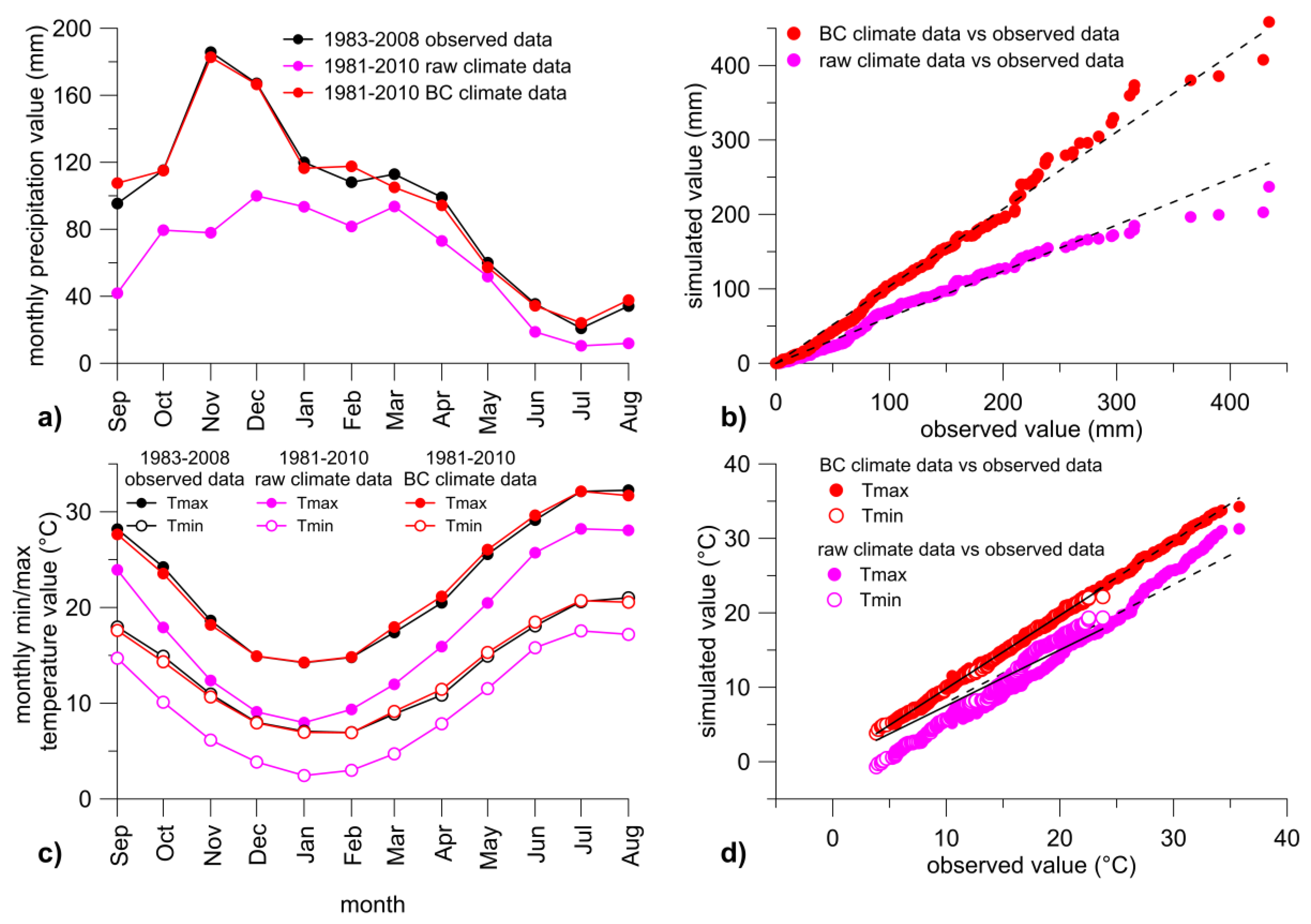
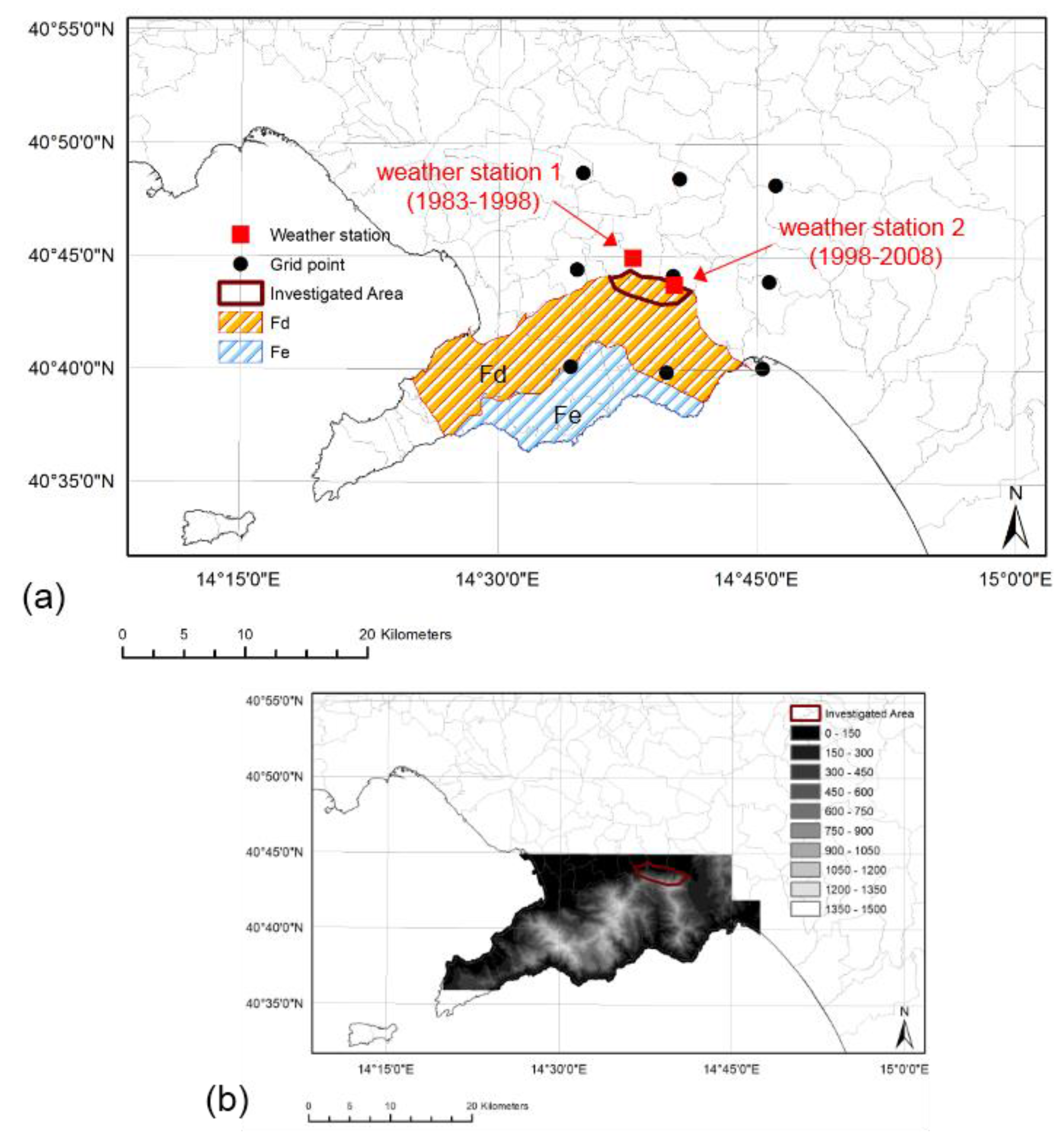
• data obtained from weather stations located very close to the slopes investigated in Nocera Inferiore town (Figure 1); specifically, the first one, included in the Servizio Idrografico e Mareografico Nazionale (SIMN, Hydrographic and Tidal National Service) network was located at about 3 km from the most affected areas and it recorded daily precipitation and the maximum and minimum temperatures from 1950 to 1999. After a fatal event in 1997, another weather station with hourly resolution was installed at the foot of the hill slopes rising behind Nocera Inferiore. This weather station collected weather values during the timespan ranging from 1 January 1998 to 1 November 2008. Unfortunately, the dataset provided by the first weather station is not complete due to occasional malfunctions and out of order (e.g., on 1981–1982 time window). Thus, assuming as the current reference time window 1981–2010, the data do not cover the entire period, but only from 1983 to 2008 (two landslide events occurred in the area during this period). Moreover, proper checks about the reliability and homogeneity of resulting time series have been carried out through SNHT and RH test ([25,26]) to evaluate the presence of breakpoints while, for the absence of statistically significant trends, Mann-Kendall test has been performed.
• simulated data provided by the bias corrected dynamical downscaled climate simulation chain (CSC) ([27,28]), presented below, on 1981–2010 time span. Data from the CSC refer to the mean spatial value computed on 3 × 3 grid points surrounding the area in which the weather stations were installed (Figure 1);
• projected data provided by the same CSC for two future time spans: 2021–2050 and 2071–2100 under two different scenarios of future concentrations of Greenhouse Gases, GHG, aerosols, A, and chemically active gases, CAG (GHG-A-CAG). Representative Concentration Pathways (RCPs) 4.5 and 8.5 are used as described below in detail. Moreover, the two periods are considered as representative for the short and long term climatology.

The CSC comprises four elements: (i) Representative Concentration Pathways (RCPs); (ii) General Circulation Models (GCMs); (iii) Regional Climate Models (RCMs); (iv) Bias Correction (BC) approaches.

RCPs provide assessments of future trajectories in concentrations of GHG-A-CAG resulting from land use changes and anthropic activities [2]. Assessments consistent with different socio-economic and demographic scenarios are provided as dependent in time on regular grids (about 60 km). More specifically, four scenarios are assumed as “references”: RCP2.6, RCP4.5, RCP6 and RCP8.5 where the suffix stands for the expected increase in radiative forcing in 2100 compared with the preindustrial era (1765) ([29,30]). RCPs are used as forcing for GCMs, which simulate atmospheric patterns on large spatial grid scales (currently in the order of 1 °C), today including models of sea ice, the carbon cycle, ice sheet dynamics and even atmospheric chemistry (Earth System Models, ESMs). Different investigations (e.g., [2,31]) have verified their ability to reproduce current climate conditions and the response to GHG-A-CAG variations with higher reliability for some weather variables (e.g., temperature) and less for others (e.g., precipitation). Nevertheless, current resolutions make them inaccurate at reproducing regional weather patterns. Consequently, several regional climate downscaling (RCD) techniques are proposed: limited area RCMs, empirical statistical downscaling methods, and variable and high-resolution atmospheric GCMs. All approaches use large-scale variables produced by GCMs as input to generate spatially refined climate information [32]. Even if this refinement makes it possible to accurately evaluate a remarkable fraction of weather patterns, RCD may misrepresent orography, land surface feedbacks and sub-grid processes, thus inducing biases preventing their use for impact analysis ([33,34,35,36]). To overcome this issue, different approaches, known as Bias Correction (BC) methods, have been proposed in recent years ([10,37,38]). They can be defined as statistical regression models calibrated, for current periods in order to detect and correct biases, assumed to systematically affect the climate simulations. Although the advantages, limitations and warnings regarding their adoption are widely debated in recent literature ([36,39]), they are currently recognized as a necessary stage in producing weather variables to use as inputs for impact predictive tools.

In particular, RCP4.5 and RCP8.5, representing a “midway” and a pessimistic but business as usual scenario respectively, are used in this study to estimate future concentration gases (in the historical period up to 2005, the IPCC dataset reporting observed GHG-A-CAG concentrations, 20C3M, is used). They force the GCM model, CMCC_CM [40] with a horizontal resolution of about 80 km; it is dynamically downscaled using the RCM COSMO_CLM model [41] at a horizontal resolution of 8 km, in the optimized suite on Italy carried out by Bucchignani et al. [22]. They show how, in terms of average values, the model performances are substantially in line with those achieved using ensemble approaches (e.g., EURO-CORDEX or ENSEMBLE experiments) while, in terms of extreme values, they usually perform better than the ensemble approaches also thanks to their higher resolution [42]. Lastly, model outputs are bias-corrected (BC) using an empirical quantile-mapping approach that makes use of a quantile-based transformation of distributions where “a quantile of the present day simulated distribution is replaced by the same quantile of the present-day observed distribution” [36]. This approach has proven outperforming the others for different weather variables or geographical areas ([10,37,43]).

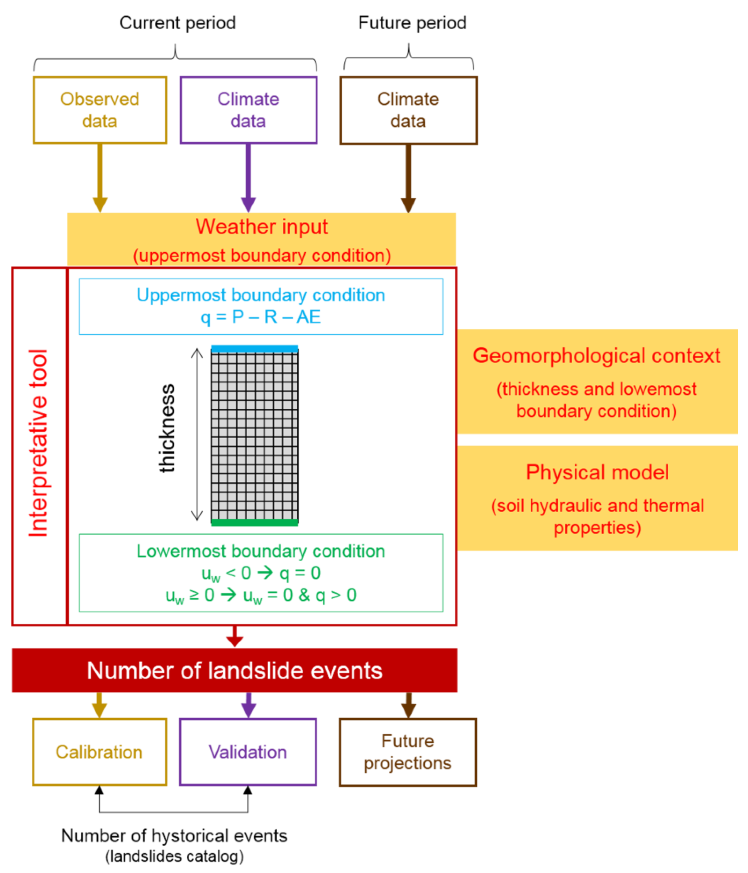
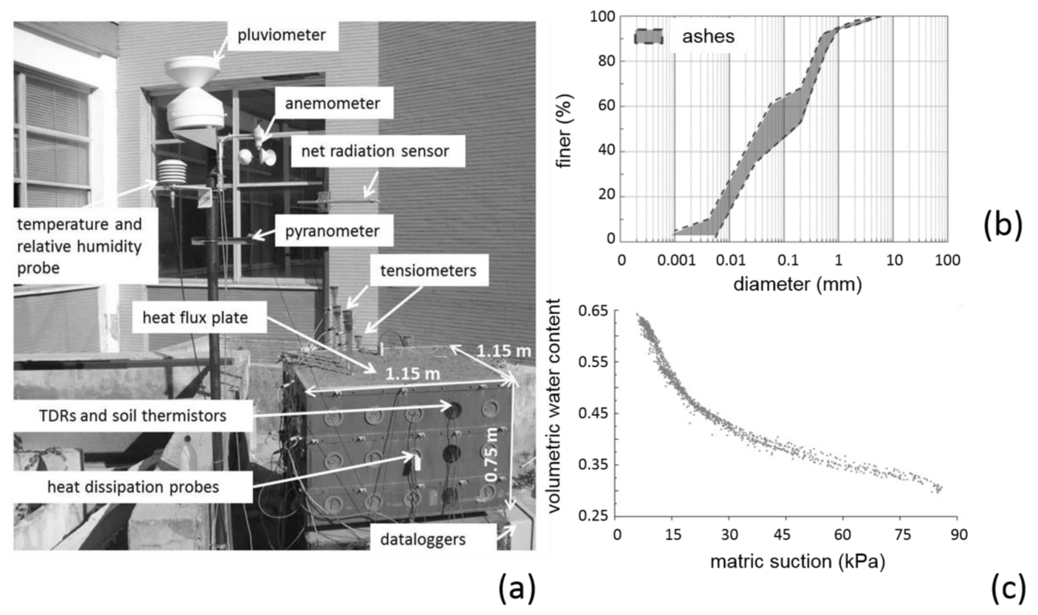
2.3. The Physical Model

A well-instrumented physical model exposed to the atmosphere (Figure 2a) was developed and monitored ([44,45]) to understand the predisposing factors and investigate the hydrological behavior of a typical pyroclastic cover under bare soil condition.

It consists of a wooden tank made of 3 cm thick boards placed on a metallic base. The tank is a parallelepiped with a square horizontal section (1.15 × 1.15 × 0.75 m). It is filled with about 1 m³ of material with a porosity of about 70%, similar to those commonly found for such covers in the field; this value was reproduced by positioning the layer using the pluvial deposition technique.

The soil investigated during the experiment is non-plastic silty sand coming from the Monteforte Irpino test site. This choice was made due to the soil’s grain size distribution (Figure 2b) that is approximately equivalent to those of the material involved in the Nocera Inferiore (southern Italy) flowslide on 4 March 2005 [16]. Mechanical and hydrological behaviors were extensively investigated through laboratory tests [46], and field monitoring of soil suction and water content [47]. Specifically, the material is cohesionless and its strength is due to a friction angle of 39°.

As for the soil-controlled boundary conditions, the lateral boundaries are impervious; moreover, the uppermost surface is left bare and the water flow considered is due to the natural interaction between soil and atmosphere. Lastly, the tank base was holed and the layer was brought into contact with a geotextile interposed between the soil layer and the holed tank base itself. From the hydraulic viewpoint, the geotextile behaves as a capillary barrier allowing drainage only at or above zero pore water pressure. Several sensors permit monitoring as atmospheric (wind, temperature, relative humidity, precipitation, net and solar radiation, soil heat flux) and soil (pore pressures, water content and soil temperature at different depths within the volume) variables.

2.4. The Interpretative Tool

The interpretative tool adopted to turn meteorological variables into hydrological soil variables related to slope stability conditions (suction and water storage) is the Wilson model ([48,49]), implemented in the Finite Element Method (FEM) code VADOSE/W 2007. It is based on the hypothesis of a rigid-soil skeleton which corresponds to neglect the effects of possible changes in soil porosity due to soil collapse upon wetting; moreover, the total stresses are considered to remain constant as far as the problems in hand are concerned (low thickness of the cover).

From the physical viewpoint, the Wilson model schematizes both liquid and vapor water flow by accounting for hydrothermal coupling and incorporates evaporation as both boundary and internal phenomenon [50]. Evaporation is quantified according to the approach suggested by [51], based on an estimation of potential evaporation using the FAO approach [52] reduced according to surface suction levels. On the other hand, the soil surface temperature, the boundary conditions of the thermal issue, is assumed equal to the temperature of the atmosphere. From this perspective it worth recalling also that the evolution of soil temperature over current and future periods are relevant for prediction of evaporative fluxes as Wilson model taking into account the effect of both internal and surface evaporation.

2.5. Conceptual Framework

The different “ingredients” introduced in previous paragraphs have been combined to obtain a conceptual framework for evaluation of potential effects of CC on landslide occurrence (Figure 3).

The analysis of geomorphological context and the monitoring and interpretation of physical model behavior was used to define geometry, lowermost boundary condition and soil parameters of the interpretative tool.

Based on these findings, a mono-dimensional domain is adopted. Such assumption has been recognized as reliable on the basis of field monitoring and sensitive analysis carried out on similar geomorphological contexts. For instance, Pirone et al. [53], interpreting in situ measurements for a pyroclastic cover during the wet season, show how seepage vectors are practically vertical towards the fractured pervious bedrock. On the other side, during the dry season the vectors are again characterized by 1D conditions although directed orthogonal to soil surface. Furthermore, again for wet season mainly interesting for the triggering of landslide events, Pagano et al. [16] compared the findings of filtration analysis carried out on 1–2D domains suggested that time-saving 1D analysis may be reliably adopted instead of 2D time-consuming for the usual bottom boundary conditions retrievable in situ.

In terms of soil properties, the interpretative tool requires a characterization of both hydraulic (soil water characteristic curve and permeability function) and thermal properties (soil thermal conductivity and volumetric specific heat). They have been assessed by referring to data provided by the physical model. Some soil properties (soil water characteristic curve and soil thermal conductivity) have been quantified merely from measurements. From this perspective, Figure 2c shows the pairs of suction and water content values measured at a depth of 15 cm from ground level. In a similar way, thermal conductivity was assessed using the heat dissipation probe and TDR measurements. Lastly, other soil properties (permeability function and volumetric specific heat) have been obtained from a trial-and-error back-analysis of the observed behavior (water storage, suction and temperature) during monitoring activity. For further details, the reader may refer to [50].

As a hydraulic bottom condition, a capillary barrier is assumed to subsist at the interface between soil and bedrock and on the basis of this assumption, impervious conditions are estimated for suction values higher than 0 kPa while for lower values water fluxes are discharged from the soil column. These conditions tend to reproduce the contrast in hydraulic permeability between the pyroclastic mantle and the highly fractured calcareous bedrock (and or pumiceous layer) [54].

As a hydraulic upper condition, the potential fluxes (precipitation and potential evaporation) derived from the six 30-year datasets of atmospheric boundary conditions (Table 1) were adopted. Regarding thermal boundary conditions, for the upper condition we assumed the soil surface temperature to be equal to the temperature of the atmosphere while, for the bottom condition we assumed a constant value of 15 °C.

Firstly, the interpretative tool was forced adopting as hydraulic upper condition the observed data available over 1983–2008. During this time span, two landslide events actually occurred (10 January 1997–4 March 2005). In correspondence of such events, the interpretative tool returns the higher values of water storage (bulk water content) along the entire soil profile (2 m). It is then adopted as proxy for landslide occurrence (calibration). So derived thresholds are maintained forcing the model through climate simulation: on 1981–2010, it allows verifying the reliability of the entire simulation chain (validation). Finally, the threshold was adopted to evaluate the potential effects of CC on landslide occurrence considering as hydraulic upper condition the BC climate data for the two RCPs over 2021–2050 and 2071–2100 (future projections).

2.6. Analysis of Uncertainties in Climate Modeling

Due to the high computational costs linked to the adoption of a physically based approach, a single modeling chain is used to force the predictive tool even though two RCPs are taken into account. However, as is well known, greater uncertainties currently affect climate modeling and the weight of contributions related to single elements of the simulation chain are often a function of the area investigated, the weather variables or season ([28,55]). On the other hand, having feedback or information about how the expected variations provided by the adopted climate chain agree or disagree from the other available SOTA climate simulations can provide valuable indications about the retrieved findings. To this end, the study considered the ten climate simulations currently available up to 2100 under RCP4.5 and RCP8.5 for the European domain within the CORDEX program (EURO-CORDEX) at a resolution of about 12 km ([56]). Data from EURO-CORDEX was elaborated computing for indicators generally assumed having higher information content in explaining landslide occurrences. To this end, the Reliability Ensemble Averaging (REA) approach proposed by [57,58] was implemented. It is based on the assumption that some models are “better” than others, and the “better” models should receive more weight when the models are combined [59]. For this reason, in this approach, reliability factor R is introduced for each model i:

$$R_i={\left[{\left(R_{b,i}\right)}^m{\left(R_{d,i}\right)}^n\right]}^{\frac{1}{mn}}={\left[{\left(\frac{{\epsilon }_T}{abs\left(B_{T,i}\right)}\right)}^m{\left(\frac{{\epsilon }_T}{abs\left(D_{T,i}\right)}\right)}^n\right]}^{\frac{1}{mn}}$$

(1)

$R_{b,i}$ measures the model’s reliability as a function of model bias $B_{T,i}.$

$R_{d,i}$ evaluates the model’s reliability in terms of distance $D_{T,i}$ of the change calculated by a given model from the REA average change.

${\epsilon }_T$ assesses natural variability; here, it is computed through a bootstrapping approach for 1000 iterations, as the standard error of the average value of the observed indicator; the exponents m and n serve as relative weight for the two contributions.

Tebaldi et al. [60] and Smith et al. [61] demonstrate how assumptions on which a heuristic REA approach is based can be traced back to a more rigorous Bayesian approach. In accordance with [57] and [58], the REA average does not represent actual climate response to climate forcing scenarios; however, the REA average represents the best estimate of this response.

The probability of a climate change exceeding a certain threshold $\Delta {\mathrm{X}}_{\mathrm{th}}$ is given by the weighted sum of all reliability factors associated to models for which an equal or higher anomaly value is returned:

$$P_{m\Delta X_{th}}={{\displaystyle \sum }}_i{P}_{mi}={{\displaystyle \sum }}_i\frac{R_i}{{{\displaystyle \sum }}_{i=1}^n{R}_i}\Delta X_i\ge \Delta X_{th}$$

(2)

3. Results and Discussion

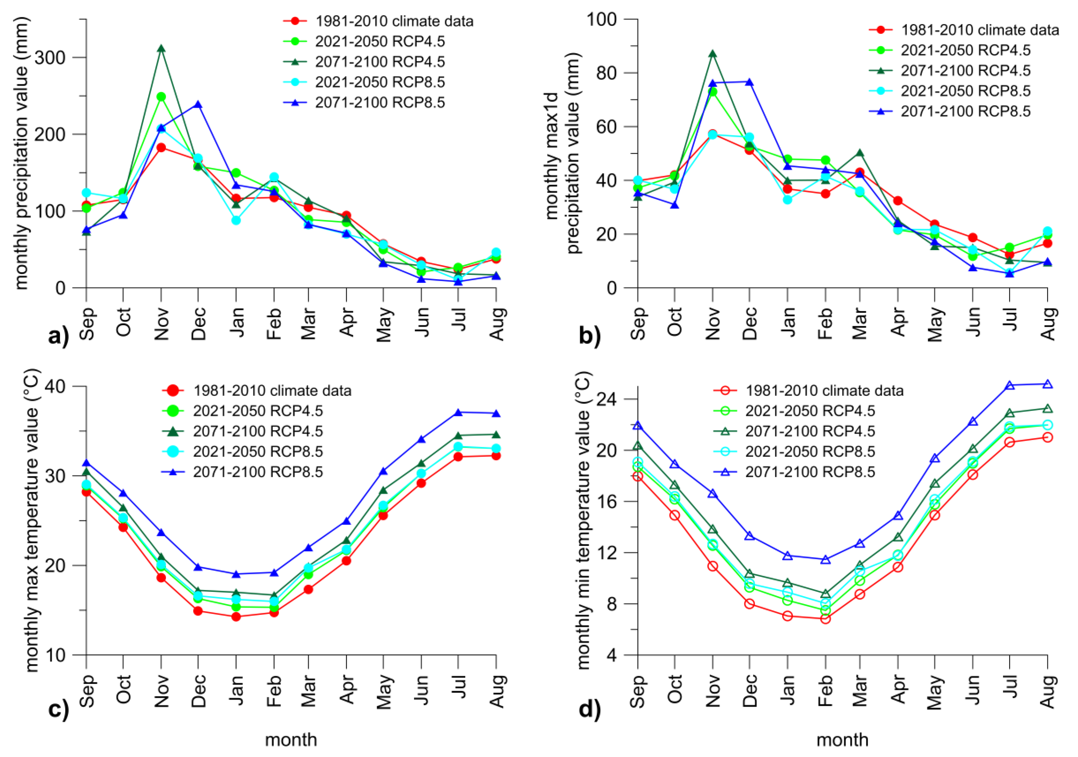
3.1. Climate Projections

Figure 4a–c shows the monthly precipitation values and the min/max temperatures observed or returned by raw and bias-corrected climate modeling for the current period. From the observations, weather patterns typical of the Mediterranean area clearly arise.

Seasonal temperature patterns return higher values in JJA with maximum temperatures exceeding 32 °C, while minimum values, ranging from 5 °C to 10 °C, are registered in DJF. On the other hand, two distinct periods, respectively wet and dry, can clearly be recognized: the first one approximately coincides with autumn and winter, and the second one includes the other months. Higher cumulative precipitation values are observed in November and December (160–200 mm). As for findings from a raw CSC, they are able to replicate seasonal patterns in a satisfactory way but with substantial underestimations for both weather variables; however, the adoption of BC approaches permits a significant reduction of biases over the entire year. From this perspective, the results depicted in Figure 4b,d result very interesting. In them, for the period 1983–2008, monthly precipitation (Figure 4b) and max/min temperature (Figure 4d) observed and returned by raw/bias corrected data are sorted and compared. Observed and bias corrected data are characterized by highly satisfying values of correlation coefficients: 1.03 for precipitation (R² = 0.99), 0.99 per T_max (R² ~ 1) and 0.98 per T_min (R² ~ 1). On the other side, several deficiencies currently making the adoption of bias correction approaches necessary, are revealed by the comparison between observed and raw climate data; in this case, correlation coefficients are 0.62 for precipitation (R² = 0.97), 0.79 for maximum temperature (R² = 0.90) and 0.75 for minimum temperature (R² = 0.89).

In terms of climate projections, substantial increases in temperature are assessed (Figure 5c,d): for RCP4.5, they are, on average, 1.5 °C for a close time horizon and in the long term, between 2.8 °C (wet season) and 3.5 °C (dry season). These increases are exacerbated for RCP8.5 with values of approximately 2 °C for 2021–2050 and 5–6 °C for 2071–2100. On the other hand, for precipitation, Figure 5a,b shows the monthly cumulative and daily maximum values. For the first, large increases are estimated in November under RCP4.5 where it attains values about equal to 135% and 170% compared to the actual ones respectively on short and long time horizon while, under RCP8.5, the largest variations are estimated for November (114%) and December (about 150%) on 2071–2100 time window. Conversely, substantial decreases, a consequence of the time horizon and the severity of the RCPs, are estimated during the dry season (up to −50/60%). Similar conclusions can be drawn for daily maximum values even if the increases during the wet season (Nov–Feb) are often estimated for both RCPs and/or time horizons (only in January are values lower than the current ones simulated for RCP4.5 in 2021–2050).

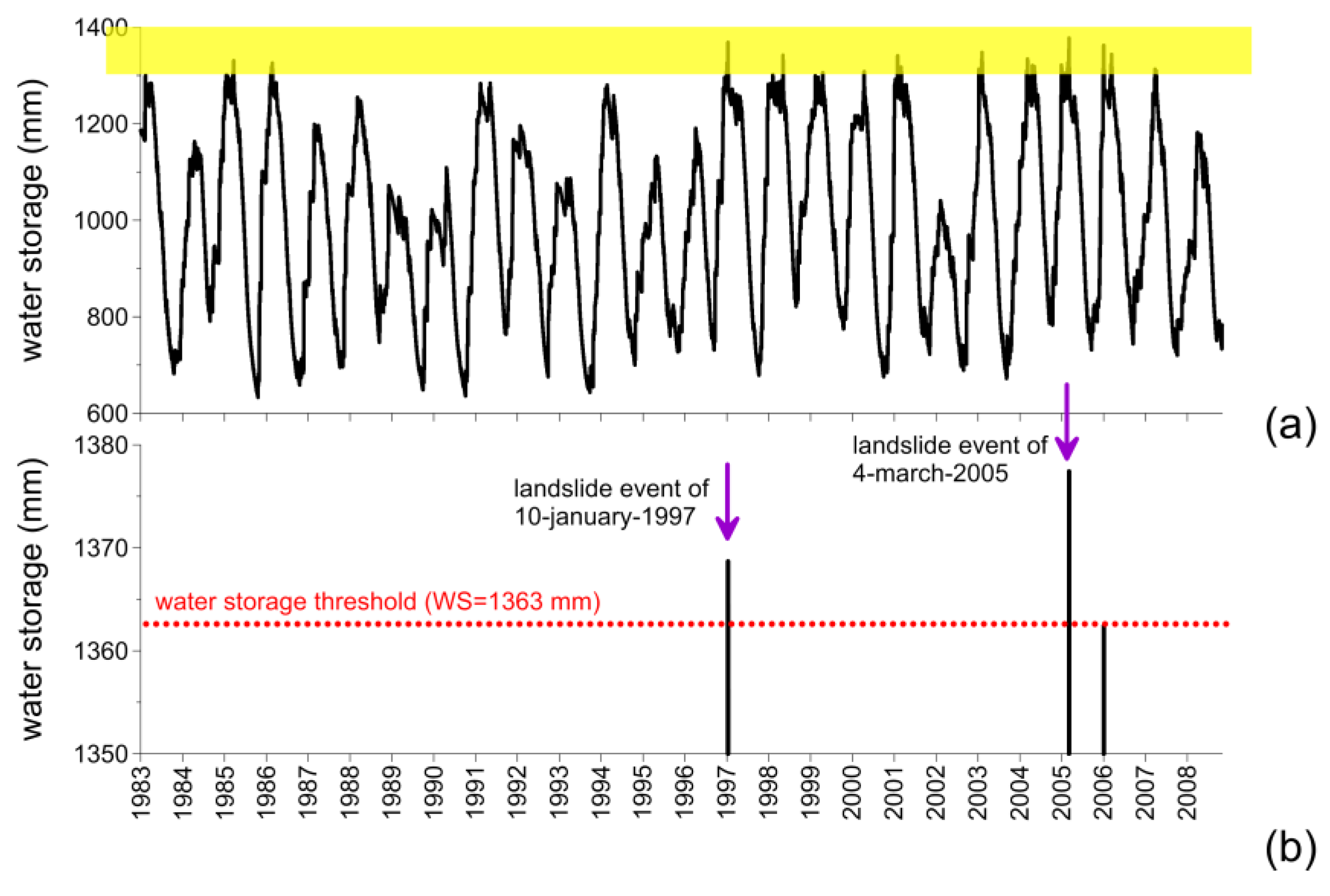
3.2. Definition of a Landslide Physically-Based Threshold (Calibration)

The calibrated thermo-hydraulic interpretative tool was adopted to reinterpret the history of the observed weather patterns, available for the years 1983–2008 in terms of pore water pressures and water storage, which were assumed as proxies to detect conditions prone to slope instability. The aim is to retrieve a physically based threshold capable of reproducing landslide events actually occurred, minimizing the number of false alarms.

Figure 6 shows the evolution of water storage estimated for the observation period. Of course, it follows a seasonal pattern driven by the weather conditions discussed in 2.2 with two clearly recognizable periods: October–March, characterized by wet and cold conditions and April to September, where opposite conditions are observed. Nevertheless, great interannual variation can be observed for both minimum and maximum values. The minimum values, obtained at the end of the dry season, range from between 650 mm and 800 mm (the degree of bulk saturation ranges from 0.45 to 0.6); on the other hand, the maximum values, reached in the second part of the wet season, display a more accentuated spread: in ten out of twenty-six hydrological years, peak values much lower than 1200 mm are reached (with a bulk saturation degree approximately equal to 0.85) while in ten other cases, they exceed 1300 mm (with a bulk saturation degree approximately equal to 0.9). However, the maximum values, highlighted in Figure 6b, are attained for the weather patterns that induced the two landslide events that occurred during the observation period, namely 10 January 1997 and 4 March 2005. Then, for the sake of simplicity, the water storage threshold determining the potential occurrence of landslides can be fixed at the first peak for which landslide events did not occur; this value is 1363 mm (about 97%). Nevertheless, no other values higher than 1350 mm are estimated throughout the entire weather history. It should be stressed that, using such thresholds, no assumptions are formulated about the triggering mechanism; furthermore, it entails substantial simplifications for soil water pore pressure distributions inducing the event, and details about the sliding surface cannot be obtained.

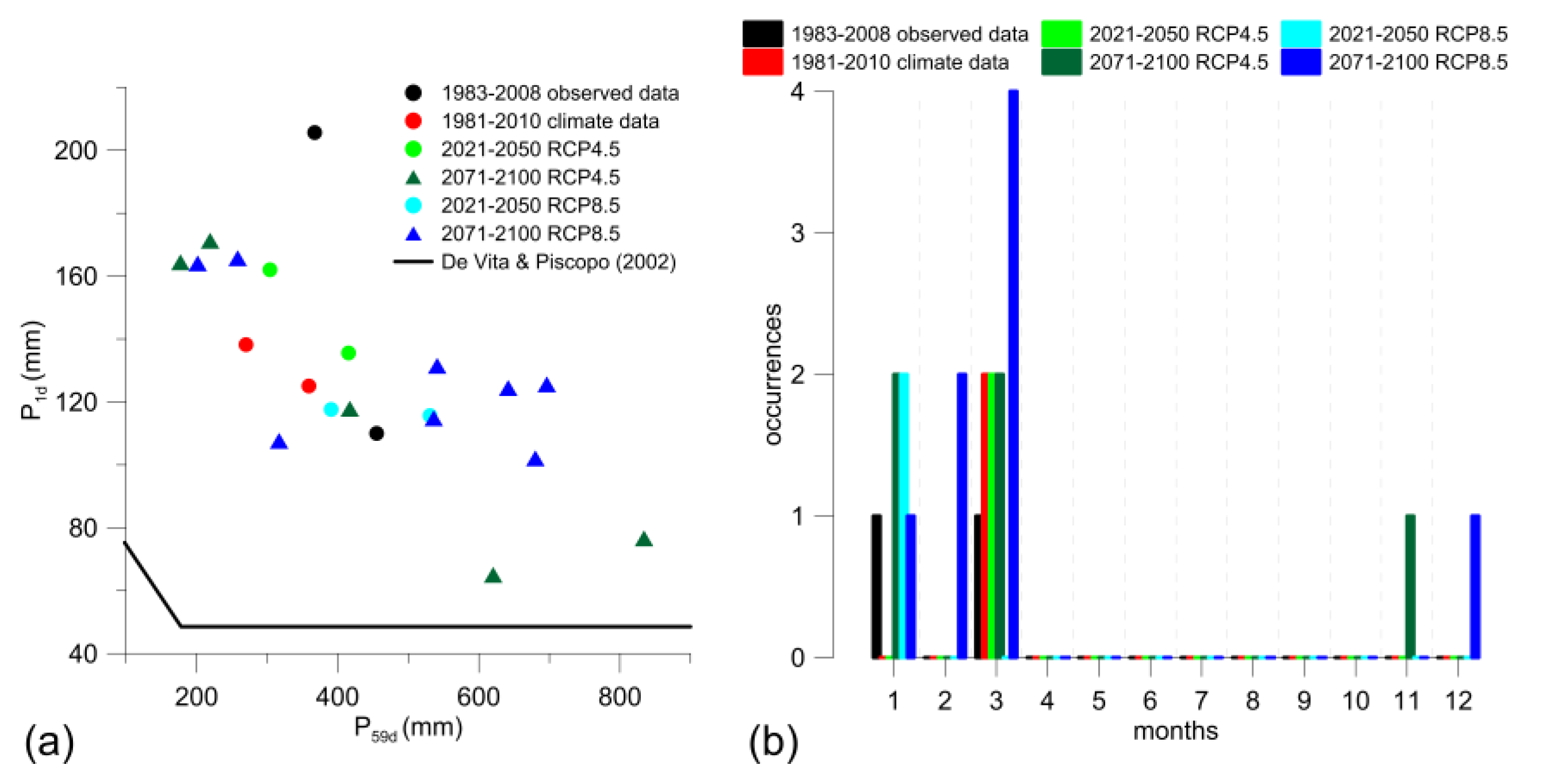
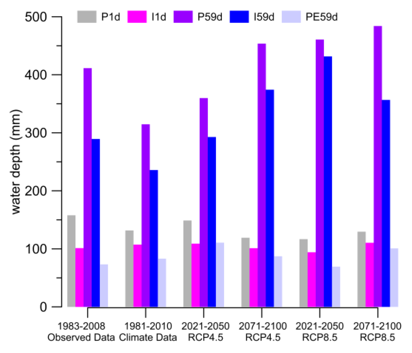
3.3. Validation of Simulation Chain and Landslide Projections over Future Periods

Weather patterns for which estimations are made for exceeding the water storage threshold (Figure 6) using the interpretative tool are reported in Figure 7a in terms of precipitation observed on the day of occurrence, P_1d and cumulative precipitation over the previous 59 days, P_59d. They are assumed as synthetic indicators (proxies) for landslide occurrence in pyroclastic covers of Lattari Mountains; in the specific, the first one tends to account for the effect of “precipitation triggering event” that could be even characterized by longer duration while the second one tends to summarize the effect of antecedent conditions. The pairs of points P_1d-P_59d are shown for both observed and simulated (bias corrected) data for current and future time spans. For the current time window, the interpretative tool driven by climate simulation data returned the same number of occurrences (two events, red dots in Figure 7a) as were actually verified and returned using forcing observations (black dots in Figure 7a); however, in these cases, potential conditions for landslide occurrence are reached with lower P₁ and P₅₉ values. In the short term (2021–2050), no variations were detected (two events) for either RCPs; furthermore, for both indicators the occurrence is estimated in association with values close to those for current conditions. On the other hand, on the farthest time horizon, a substantial increase in number of potential events was returned: five events under RCP4.5 and eight under RCP8.5. For the “middle-way” scenario, occurrences are associated in two cases with high P_1d values and in two other cases with P_59d much higher than those estimated for the current time window (in the remaining case, the values are similar to those for the present time window of reference). Lastly, for a more pessimistic scenario, in two cases, once more, potential occurrence is associated with a particularly high P_1d value and in five cases with P_59d values higher than those for current conditions. Nevertheless, in any case, P_1d reaches or exceeds the value observed on the day of 4 March 2005 (205.6 mm).

In order to investigate the factors might regulate future expected increase, Figure 8 shows the average values associated to potential failure events every 30 years for the observed data and climate simulations, and the estimated infiltration rate for the two previous indicators (P_1d, P_59d) on the day of potential occurrence (I_1d) and the previous 59 days (I_59d). The cumulative potential evaporation over the previous 59 days (PE_59d) is also given. Comparison between the first two bar groups related to the observed and modeled data on current periods displays how, using forcing modeled data, somewhat lower values in precipitation patterns are, on average, required to achieve slope failure conditions. For projections, the increase in cumulative antecedent values seems to have a greater influence on expected growth in occurrences. Indeed, while the precipitation intensity (and associated infiltration rates) estimated for the triggering day have values comparable to those in the current period, the mean future P_59d values are considerably higher. In particular, under RCP8.5 and on long time horizon for RCP4.5 they exceed 450 mm with infiltration rates of approximately 350–400 mm while for the other cases they are lower than 300 mm. Finally, on average, PE_59d does not display significant variations between current and future periods given also the particularly wet conditions required for exceeding the water content threshold.

Figure 9 shows the expected variations in maximum cumulated precipitations for 1 and 59 days. They are calculated using the Generalized Extreme Value (GEV) approach on observed and modeled bias-corrected data. In this respect, it is worth recalling that the greater the spread between the investigated return time period and the time window used for GEV parameter calibration, the higher the uncertainties associated with evaluation ([62,63]). Both graphs show similar patterns: increases are strictly related to the time horizon but, while differences are contained for RCP4.5, they are very pronounced for RCP8.5, with values on the short time horizon comparable to those in the current period and values for the long time horizon well above all the others. Moreover, it is worth noting that, despite the adoption of a bias correction approach, biases persist for daily values between curves estimated from observed and modeled precipitation values while a better representation of observed conditions is returned for the longer time P_59d. However, the trends confirm a potential worsening of slope stability conditions in the investigated area.

3.4. Comparison between Empirical and Physically-Based Thresholds

The P_1d and P_59d proxies adopted as indicators for landslide occurrence in 3.3 are analogous to those adopted by De Vita & Piscopo [64] defining an empirical threshold for the same geomorphological context (see Figure 7a) and adopted as reference in previous work [21] to assess through expeditious approaches the potential effect of climate changes on landslide occurrence.

Therefore, it is interesting to compare the findings provided by the interpretative tool with those of [21] (Table 1). The same observation dataset and climate simulations are utilized also here. In previous work, the “likelihood of success”, representing the ratio between the number of landslides actually occurred (2 events) and the number of pairs of points P_1d-P_59d (70 events) exceeding the thresholds, is estimated for the observed dataset (likelihood of success = 2.9%) and applied to findings provided by climate simulations. Comparing empirical and physically-based thresholds, two main differences arise: firstly, using the empirical threshold, less remarkable increases are estimated especially on the farthest time; in the worst case (RCP4.5 2071–2100), the number of potential failure events is about 3.6 for 30 years while, using a physically-based approach, it rises to eight (RCP8.5 2071–2100). Secondly, if only cumulative values are considered (

Table 2. For both RCPs (first column) and time horizons (second), the number of potential events estimated using the De Vita & Piscopo [64] threshold (third), seasonal distribution (fourth to seventh), and potential failure events obtained using the “likelihood of success” estimated for the observed data from 1983 to 2008.

Concentration Scenario	Time Horizon	Precipitation Events Exceeding the Threshold	DJF	MAM	JJA	SON	Potential Failure Events
RCP4.5	2021–2050	109	50	8	1	50	3.11
	2071–2100	125	51	16	0	58	3.57
RCP8.5	2021–2050	90	49	9	1	31	2.57
	2071–2100	119	72	9	0	38	3.40

), higher increases are estimated under RCP4.5 while the opposite occurs for more complex approaches. Some possible explanations for these differences arise from a comparison between expected monthly distribution of potential events during the year provided by the thermo-hydraulic approach (Figure 7b) and seasonal variations supplied by using the empirical threshold (Table 2). The latter concentrates the main part of the expected events in Winter (40–60%) and Autumn (30–46%); a considerably lower number is estimated as potentially occurring in Spring (7–13%) while in Summer, two rainfall histories (for both RCPs) entail threshold crossing in the term. On the other hand, physically based approaches return conditions of potential failure clustered in the January-March time span; the two events that occurred are correctly identified while, using a climate simulation chain for the current period, the two potential events take place in March. For future time spans, similarly, only two events fall outside the Jan-March time window: November for RCP4.5 and December for RCP8.5, both on the farthest term horizon. In this regard, this event distribution indicates how reaching the water content threshold can be profoundly influenced by several factors disregarded or not properly taken into account by the empirical approach: (i) the actual rainfall history (i.e., sequence of wet and dry days) mainly regulating the real infiltration rates within the soil; in this respect, not all heavy rainfall events were able to be fully absorbed, contributing to increased soil water content; (ii) in the Mediterranean context, evaporation losses may remove a remarkable amount of water during most of the year; moreover, in future time spans, the expected increase in temperature could raise the atmospheric demand although the actual outgoing fluxes are also a main function of soil water availability; (iii) nevertheless, the adoption of P_59d as a proxy could underestimate the length of the effective antecedent time window. For similar geomorphological contexts, Pagano et al. [16] propose four months as an effective time window while Rossi & Chirico [65] use cumulative rainfall for the hydrological year as proxy. Nevertheless, apart from the two events that occurred in the period from 1983–2008, three more events were recorded in Nocera Inferiore: in two cases in late Autumn (1960, 1961) and again in March (1972) for the other one. Then, in the physically based approach, explicitly taking account of such hydrological dynamics, the time window is tightened in the second part of the wet season during which the effect of antecedent precipitation became relevant while, at the same time, the influence of evaporative losses is less prominent. Moreover, in terms of seasonality, climate changes could induce a shift towards the final part of the wet season with 10 out of 15 potential future events between February and March.

3.5. The Role of Uncertaintes in Climate Projections

In Figure 10, comparison between the expected variation in P_1d and P_59d returned by the CSC (on the x-axis) implemented in this work and those provided by the EURO-CORDEX ensemble in terms of cumulative exceedance probability (cep) are illustrated for the two time horizons and RCPs. The cumulative exceedance probability (cep) was computed through the Reliability Ensemble Averaging (REA) introduced in 2.6. Also in this case, for every model, 3 × 3 grid points surrounding the weather station were selected. All simulations have been bias-corrected using the same approach explained in 2.2. For RCP4.5, the variations assessed in the area by the adopted CSC are characterized by low probabilities of exceedance: <10% for 2021–2050 and about 15% for 2071–2100 for P_1d and <10% for both periods for P_59d. Similar results are estimated for RCP8.5 on the long time horizon while for 2021–2050, they do not exceed 85% and 40% respectively for P_1d and P_59d. Such results also help framing the previous trends more clearly: in particular, bearing in mind current uncertainties on future projections, the variations generally detected in the area by the adopted CSC are somewhat higher than the ensemble mean values retrieved using EURO-CORDEX simulations (except for RCP8.5 on 2021–2050) potentially resulting in heavier estimates for future changes in landslide occurrences.

4. Conclusions

This work attempts to provide an assessment of future variations of landslide events involving pyroclastic covers in the Campania region, under the potential effect of CC. The case study is particularly interesting as the hydraulic behavior of the soils involved are “intermediate” between coarse and fine formations as for the location of slopes in the Mediterranean area, considered a hot-spot for climate changes.

The analyses reveal how increased hazardous conditions could be expected with different features according to the time horizon and RCPs investigated. Moreover, the adoption of a physically-based approach as an interpretative tool, able to properly investigate soil-atmosphere interaction, allows a reduction in the “number of false alarms” when forced by weather observations and improving the representation of seasonal patterns for the events. Through this approach, it appears clearly how an increase in cumulative values during the wet season could act as a main forcing element in the increase of landslide events. Nevertheless, also an increase in the magnitude and occurrence of heavy rainfall events on a daily scale is expected. Finally, the expected variations in precipitation values assumed as proxies for the landslide events returned by the adopted climate modeling chain (at 8 km) are compared to those obtained by the EURO-CORDEX ensemble currently representing the ensemble at the highest resolution (12 km) available for the area.

However, assumptions and uncertainties should be clearly kept in mind:

-

a time-saving 1D approach is preferred; although the reliability of such choice is supported by different studies (2.4), however, it could entail also substantial misrepresentations mainly in intermediate seasons;

-

the analysis does not account for the benefic role of vegetation reducing the infiltrated precipitation and increasing, at the same time, the water amount released in atmosphere through transpiration dynamics;

-

also if Wilson model is largely and successfully adopted in geotechnical field, it requires several simplifications that should be stressed; among the others, the soil surface temperature and the boundary conditions of the thermal issue are assumed to be equal to the temperature of the atmosphere;

-

climate simulation chain are currently affected by substantial uncertainties; they are partially taken into account through ensemble approaches in which the same impact tool is forced by the different components of an ensemble of models; however, due to heavy computational burden required by the adoption of used CSC, a simplified evaluation of uncertainties in potential variation of weather forcing is carried out in terms of weather patterns recognized as “proxies” for attainment of slope failure conditions. In this respect, the approach could easily be replicated also for other test cases or impact studies.

References

1. World Meteorological Organization. The Global Climate in 2011–2015; WMO-No. 1179; World Meteorological Organization: Geneva, Switzerland, 2016. [Google Scholar]
2. Intergovernmental Panel on Climate Change. Climate Change 2014: Synthesis Report. In Contribution of Working Groups I, II and III to the Fifth Assessment Report of the Intergovernmental Panel on Climate Change; Intergovernmental Panel on Climate Change: Geneva, Switzerland, 2014; p. 151. [Google Scholar]
3. Seneviratne, S.I.; Nicholls, N.; Easterling, D.; Goodess, C.M.; Kanae, S.; Kossin, J.; Luo, Y.; Marengo, J.; McInnes, K.; Rahimi, M.; et al. (Eds.) Managing the Risks of Extreme Events and Disasters to Advance Climate Change Adaptation. A Special Report of Working Groups I and II of the Intergovernmental Panel on Climate Change (IPCC); Cambridge University Press: Cambridge, UK; New York, NY, USA, 2012; pp. 109–230. [Google Scholar]
4. Wu, X.; Chen, X.; Zhan, F.B.; Hong, S. Global research trends in landslides during 1991–2014: A bibliometric analysis. Landslides 2015, 1–12. [Google Scholar] [CrossRef]
5. Gariano, S.L.; Guzzetti, F. Landslides in a changing climate. Earth-Sci. Rev. 2016. [Google Scholar] [CrossRef]
6. Soldati, M.; Corsini, A.; Pasuto, A. Landslides and climate change in the Italian Dolomites since the Late glacial. Catena 2004, 55, 141–161. [Google Scholar] [CrossRef]
7. Jaedicke, C.; Solheim, A.; Blikra, L.H.; Stalsberg, K.; Sorteberg, A.; Aaheim, A.; Kronholm, K.; Vikhamar-Schuler, D.; Isaksen, K.; Sletten, K.; et al. Spatial and temporal variations of Norwegian geohazards in a changing climate, the GeoExtreme Project. Nat. Hazards Earth Syst. Sci. 2008, 8, 893–904. [Google Scholar] [CrossRef]
8. Comegna, L.; Picarelli, L.; Bucchignani, E.; Mercogliano, P. Potential effects of incoming climate changes on the behaviour of slow active landslides in clay. Landslides 2013, 10, 373–391. [Google Scholar] [CrossRef]
9. Rianna, G.; Zollo, A.L.; Tommasi, P.; Paciucci, M.; Comegna, L.; Mercogliano, P. Evaluation of the effects of climate changes on landslide activity of Orvieto clayey slope. Procedia Earth Planet. Sci. 2014, 9, 54–63. [Google Scholar] [CrossRef]
10. Villani, V.; Rianna, G.; Mercogliano, P.; Zollo, A.L. Statistical Approaches versus Weather Generator to Downscale RCM Outputs to Slope Scale for Stability Assessment: A Comparison of Performances. Electron. J. Geotech. Eng. 2015, 20, 1495–1515. [Google Scholar]
11. Ciabatta, L.; Camici, S.; Brocca, L.; Ponziani, F.; Stelluti, F.; Berni, N.; Moramarco, T. Assessing the impact of climate-change scenarios on landslide occurrence in Umbria Region, Italy. J. Hydrol. 2016. [Google Scholar] [CrossRef]
12. Ciervo, F.; Rianna, G.; Mercogliano, P.; Papa, M.N. Effects of climate change on shallow landslides in a small coastal catchment in southern Italy. Landslides 2016. [Google Scholar] [CrossRef]
13. Borgatti, L.; Soldati, M. Landslides as a geomorphological proxy for climate change: A record from the Dolomites (northern Italy). Geomorphology 2010, 120, 56–64. [Google Scholar] [CrossRef]
14. Rianna, G.; Comegna, L.; Mercogliano, P.; Picarelli, L. Potential effects of climate changes on soil–Atmosphere interaction and landslide hazard. Nat. Hazards 2016. [Google Scholar] [CrossRef]
15. Dixon, N.; Brook, E. Impact of predicted climate change on landslide reactivation: Case study of Mam Tor, UK. Landslides 2007, 4, 137–147. [Google Scholar] [CrossRef]
16. Pagano, L.; Picarelli, L.; Rianna, G.; Urciuoli, G. A simple numerical procedure for timely prediction of precipitation-induced landslides in unsaturated pyroclastic soils. Landslides 2010, 7, 273–289. [Google Scholar] [CrossRef]
17. Ferlisi, S.; De Chiara, G.; Cascini, L. Quantitative risk analysis for hyperconcentrated flows in Nocera Inferiore (southern Italy). Nat. Hazards 2015, 81 (Suppl. 1), 89–115. [Google Scholar] [CrossRef]
18. Santini, M.; Valentini, R. Predicting hot-spots of land use changes in Italy by ensemble forecasting. Reg. Environ. Chang. 2011, 11, 483–502. [Google Scholar] [CrossRef]
19. Guiot, J.; Cramer, W. Climate change, the Paris Agreement thresholds and Mediterranean ecosystems. Science 2016, 354, 4528–4532. [Google Scholar] [CrossRef] [PubMed]
20. Damiano, E.; Mercogliano, P. Potential effects of climate change on slope stability in unsaturated pyroclastic soils. In Landslide Science and Practice; Springer-Verlag Berlin: Heidelberg, Germany, 2013; Volume 4, pp. 15–25. [Google Scholar]
21. Reder, A.; Rianna, G.; Mercogliano, P.; Pagano, L. Assessing the Potential Effects of Climate Changes on Landslide Phenomena Affecting Pyroclastic Covers in Nocera Area (Southern Italy). Procedia Earth Planet. Sci. 2016, 16, 166–176. [Google Scholar] [CrossRef]
22. Bucchignani, E.; Montesarchio, M.; Zollo, A.L.; Mercogliano, P. High-resolution climate simulations with COSMO-CLM over Italy: Performance evaluation and climate projections for the 21st century. Int. J. Climatol. 2015. [Google Scholar] [CrossRef]
23. Picarelli, L.; Santo, A.; Di Crescenzo, G.; Olivares, L. Macro-Zoning of Areas Susceptible to Flowslide in Pyroclastic Soils in Campania Region. In Proceedings of the 10th International Symposium on Landslides, Xi’an, China; Chen, Z., Zhang, J., Li, Z., Wu, F., Ho, K., Eds.; Taylor & Francis: London, UK, 2008; pp. 1951–1958. [Google Scholar]
24. Budetta, P.; de Riso, R. The Mobility of Some Debris Flows in Pyroclastic Deposits of the Northwestern Campanian Region (Southern Italy). Bull. Eng. Geol. Environ. 2004, 63, 293–302. [Google Scholar] [CrossRef]
25. Wang, X.L.; Wen, Q.H.; Wu, Y. Penalized maximal t test for detecting undocumented mean change in climate data series. J. Appl. Meteorol. Climatol. 2007, 46, 916–931. [Google Scholar] [CrossRef]
26. Wang, X.L. Penalized maximal F-test for detecting undocumented mean shifts without trend-change. J. Atmos. Ocean. Tech. 2008, 25, 368–384. [Google Scholar] [CrossRef]
27. Zollo, A.L.; Mercogliano, P.; Turco, M.; Vezzoli, R.; Rianna, G.; Bucchignani, E.; Manzi, M.P.; Montesarchio, M. Architectures and Tools to Analyse the Impact of Climate Change on Hydrogeological Riskon Mediterranean Area. Available online: http://www.cmcc.it/pubblicazioni/pubblicazioni/research-papers/rp0129-isc-03-201220 (accessed on 2 June 2012).
28. Mercogliano, P.; Segoni, S.; Rossi, G.; Sikorsky, B.; Tofani, V.; Schiano, P.; Catani, F.; Casagli, N. Brief communication “A prototype forecasting chain for rainfall induced shallow landslides”. Nat. Hazards Earth Syst. Sci. 2013, 13, 771–777. [Google Scholar] [CrossRef]
29. Moss, R.H.; Edmonds, J.A.; Hibbard, K.A.; Manning, M.R.; Rose, S.K.; van Vuuren, D.P.; Carter, T.R.; Emori, S.; Kainuma, M.; Kram, T.; et al. The next generation of scenarios for climate change research and assessment. Nature 2010, 463, 747–756. [Google Scholar] [CrossRef] [PubMed]
30. Van Vuuren, D.P.; Edmonds, J.; Kainuma, M.; Riahi, K.; Thomson, A.; Hibbard, K.; Hurtt, G.C.; Kram, T.; Krey, V.; Lamarque, J.-F.; et al. The representative concentration pathways: An overview. Clim. Chang. 2011, 109, 5–31. [Google Scholar] [CrossRef]
31. Breugem, W.P.; Hazeleger, W.; Haarsma, R.J. Mechanisms of northern tropical Atlantic variability and response to CO2 doubling. J. Clim. 2007, 20, 2691–2705. [Google Scholar] [CrossRef]
32. Giorgi, F.; Gutowski, W.J. Coordinated Experiments for Projections of Regional Climate Change. Curr. Clim. Chang. Rep. 2016. [Google Scholar] [CrossRef]
33. Christensen, J.H.; Christensen, O.B. A summary of the PRUDENCE model projections of changes in European climate by the end of this century. Clim. Chang. 2007, 81 (Suppl. 1), 7–30. [Google Scholar] [CrossRef]
34. Kotlarski, S.; Keuler, K.; Christensen, O.B.; Colette, A.; Déqué, M.; Gobiet, A.; Goergen, K.; Jacob, D.; Lüthi, D.; van Meijgaard, E.; et al. Regional climate modeling on European scales: A joint standard evaluation of the EURO-CORDEX RCM ensemble. Geosci. Model Dev. 2014, 7, 1297–1333. [Google Scholar] [CrossRef]
35. Maraun, D.; Widmann, M.; Gutiérrez, J.M.; Kotlarski, S.; Chandler, R.E.; Hertig, E.; Wibig, J.; Huth, R.; Wilcke, R.A.I. VALUE: A framework to validate downscaling approaches for climate change studies. Earth’s Future 2015, 3, 1–14. [Google Scholar] [CrossRef]
36. Maraun, D. Bias Correcting Climate Change Simulations—A Critical Review. Curr. Clim. Chang. Rep. 2016. [Google Scholar] [CrossRef]
37. Teutschbein, C.; Seibert, J. Bias correction of regional climate model simulations for hydrological climate change impact studies: Review and evaluation of different methods. J. Hydrol. 2012, 456–457, 12–29. [Google Scholar] [CrossRef]
38. Lafon, T.; Dadson, S.; Buys, G.; Prudhomme, C. Bias correction of daily precipitation simulated by a regional climate model: A comparison of methods. Int. J. Climatol. 2013, 33, 1367–1381. [Google Scholar] [CrossRef]
39. Ehret, U.; Zehe, E.; Wulfmeyer, V.; Warrach-Sagi, K.; Liebert, J. Should we apply bias correction to global and regional climate model data? Hydrol. Earth Syst. Sci. 2012, 16, 3391–3404. [Google Scholar] [CrossRef]
40. Scoccimarro, E.; Gualdi, S.; Bellucci, A.; Sanna, A.; Fogli, P.; Manzini, E.; Vichi, M.; Oddo, P.; Navarra, A. Effects of Tropical Cyclones on Ocean Heat Transport in a High Resolution Coupled General Circulation Model. J. Clim. 2011, 24, 4368–4384. [Google Scholar] [CrossRef]
41. Rockel, B.; Will, A.; Hense, A. The regional Climate Model COSMO-CLM (CCLM). Meteorol. Z. 2008, 17, 347–348. [Google Scholar] [CrossRef]
42. Zollo, A.L.; Rillo, V.; Bucchignani, E.; Montesarchio, M.; Mercogliano, P. Extreme temperature and precipitation events over Italy: Assessment of high-resolution simulations with COSMO-CLM and future scenarios. Int. J. Climatol. 2015. [Google Scholar] [CrossRef]
43. Gudmundsson, L.; Bremnes, J.B.; Haugen, J.E.; Engen Skaugen, T. Technical Note: Downscaling RCM precipitation to the station scale using statistical transformations—A comparison of methods. Hydrol. Earth Syst. Sci. 2012, 9, 6185–6201. [Google Scholar] [CrossRef]
44. Rianna, G.; Pagano, L.; Urciuoli, G. Investigation of soil-atmosphere interaction in pyroclastic soils. J. Hydrol. 2014, 510, 480–492. [Google Scholar] [CrossRef]
45. Rianna, G.; Pagano, L.; Urciuoli, G. Rainfall patterns triggering shallow flowslides in pyroclastic soils. Eng. Geol. 2014, 174, 22–35. [Google Scholar] [CrossRef]
46. Nicotera, M.V.; Papa, R.; Urciuoli, G. An experimental technique for determining the hydraulic properties of unsaturated pyroclastic soils. Geotech. Test J. 2010, 33, 263–285. [Google Scholar]
47. Pirone, M.; Papa, R.; Nicotera, M.V.; Urciuoli, G. Soil water balance in an unsaturated pyroclastic slope for evaluation of soil hydraulic behaviour and boundary conditions. J. Hydrol. 2015, 528, 63–83. [Google Scholar] [CrossRef]
48. Wilson, G.W. Soil Evaporative Fluxes for Geotechnical Engineering Problems. Ph.D. Thesis, University of Saskatchewan, Saskatoon, SK, Canada, 1990. [Google Scholar]
49. Wilson, G.W.; Fredlund, D.G.; Barbour, S.L. Coupled soil-atmosphere modelling for soil evaporation. Can. Geotech. J. 1994, 31, 151–161. [Google Scholar] [CrossRef]
50. Pagano, L.; Reder, A.; Rianna, G. Differences in Results Yielded by Different Approaches Adopted for the Interpretation of a Rapid Flowslide in a Pyroclastic Cover. Procedia Earth Planet. Sci. 2016, 16, 81–88. [Google Scholar] [CrossRef]
51. Wilson, G.W.; Fredlund, D.G.; Barbour, S.L. The effect of soil suction on evaporative fluxes from soil surfaces. Can. Geotech. J. 1997, 34, 145–155. [Google Scholar] [CrossRef]
52. Allen, R.G.; Pereira, L.S.; Raes, D.; Smith, M. FAO Irrigation and Drainage Paper No. 56. In Crop Evapotranspiration (Guidelines for Computing Crop Water Requirements); FAO—Food and Agriculture Organization of the United Nations: Rome, Italy, 1998; ISBN 92-5-104219-5. [Google Scholar]
53. Pirone, M.; Papa, R.; Nicotera, M.V.; Urciuoli, G. In situ monitoring of the groundwater field in an unsaturated pyroclastic slope for slope stability evaluation. Landslides 2015, 12, 259–276. [Google Scholar] [CrossRef]
54. Reder, A.; Pagano, L.; Picarelli, L.; Rianna, G. The role of the lowermost boundary conditions in the hydrological response of shallow sloping covers. Landslides 2016. [Google Scholar] [CrossRef]
55. Déqué, M.; Rowell, D.P.; Lüthi, D.; Giorgi, F.; Christensen, J.H.; Rockel, B.; Jacob, D.; Kjellström, E.; de Castro, M.; van den Hurk, B. An intercomparison of regional climate simulations for Europe: Assessing uncertainties in model projections. Clim. Chang. 2007. [Google Scholar] [CrossRef]
56. Jacob, D.; Petersen, J.; Eggert, B.; Alias, A.; Christensen, O.B.; Bouwer, L.; Braun, A.; Colette, A.; Déqué, M.; Georgievski, G.; et al. EURO-CORDEX: New High-Resolution Climate Change Projections for European Impact Research. Regional Environmental Change 2013; Springer: Berlin/Heidelberg, Germany, 2013; pp. 1–16. [Google Scholar]
57. Giorgi, F.; Mearns, L.O. Calculation of average, uncertainty range, and reliability of regional climate changes from AOGCM simulations via the “Reliability Ensemble Averaging” (REA) method. J. Clim. 2002, 15, 1141–1158. [Google Scholar] [CrossRef]
58. Giorgi, F.; Mearns, L.O. Probability of regional climate change based on the Reliability Ensemble Averaging (REA) method. Geophys. Res. Lett. 2003, 30, 2–5. [Google Scholar] [CrossRef]
59. Sham Bhat, K.; Haran, M.; Terando, A.; Keller, K. Climate Projections Using Bayesian Model Averaging and Space-Time Dependence. J. Agric. Biol. Environ. Stat. 2011, 16, 606–628. [Google Scholar] [CrossRef]
60. Tebaldi, C.; Smith, R.L.; Nychka, D.; Linda, O. Quantifying Uncertainty in Projections of Regional Climate Change: A Bayesian Approach to the Analysis of Multimodel Ensembles Technical Description of the Gibbs Sampler. J. Clim. 2004, 18, 1524–1540. [Google Scholar] [CrossRef]
61. Smith, R.L.; Tebaldi, C.; Nychka, D.; Mearns, L.O. Bayesian Modeling of Uncertainty in Ensembles of Climate Models. J. Am. Stat. Assoc. 2009, 104. [Google Scholar] [CrossRef]
62. Benson, M.A. Factors Influencing the Occurrence of Floods in a Humid Region of Diverse Terrain; U.S. Department of the Interior, Geological Survey: WA, USA, 1962.
63. Committee on Techniques for Estimating Probabilities of Extreme Floods. Techniques for Estimating Probabilities of Extreme Floods: Methods and Recommended Research; National Academy Press: Washington, DC, USA, 1988. [Google Scholar]
64. De Vita, P.; Piscopo, V. Influences of hydrological and hydrogeological conditions on debris flows in peri-vesuvian hillslopes. Nat. Hazards Earth Syst. Sci. 2002, 2, 27–35. [Google Scholar] [CrossRef]
65. Rossi, F.; Chirico, G.B. Definizione delle soglie pluviometriche d’allarme. In National Group for Defence from Hydrogeological Catastrophes—National Research Council (G.N.D.C.I.-C.N.R.); 2.38 Operative Unit, Salerno; Department of Civil Engineering, University of Salerno: Salerno, Italy, 1998. [Google Scholar]
Figure 1. (a) Focus on part of Campania Region reporting the area recognized by Picarelli et al. [23] as susceptible to landslide events for Lattari Mts, the location of investigated area, the location of weather station (red dots) and the 3 × 3 grid adopted for climate simulation (black dots); (b) representation of DTM for Lattari Mts.
Hydrology 04 00034 g001
Figure 2. (a) View of the physical prototype and the sensors utilized; (b) grain size distribution of the soils investigated; (c) Soil-Water Characteristic Curve retrieved by coupling the water content and pore pressure readings at a depth of 15 cm.
Hydrology 04 00034 g002
Figure 3. Conceptual framework for evaluation of potential effects of CC on landslide occurrence.
Hydrology 04 00034 g003
Figure 4. (a) Monthly cumulative precipitation values: observed (black), provided by a raw (magenta) or bias-corrected (red) CSC; (b) comparison between sorted time series of monthly precipitation (1983–2008) for observed vs values provided by raw (magenta) or bias-corrected (red) climate models; black dashed lines identify regression lines; (c) monthly temperature values: observed (black), provided by a raw (pink) or bias-corrected (red) CSC; minimum temperatures are represented by white dots, and the maximum by filled dots; (d) comparison between sorted time series of monthly temperature (1983–2008) for observed vs values provided by raw (magenta) or bias-corrected (red) climate models; filled dots are used for maximum temperature and white dots for minimum temperature black dashed (continuous) lines identify regression lines for maximum temperature.
Hydrology 04 00034 g004
Figure 5. (a) Monthly cumulative precipitation values provided by a bias-corrected CSC for 1981–2010 (red), 2021–2050 RCP4.5 (light blue), 2071–2100 RCP4.5 (dark blue), 2021–2050 RCP8.5 (light green), and 2071–2100 RCP8.5 (dark green); (b) the same for monthly max 1d precipitation; (c) the same for monthly mean max temperature; (d) the same for monthly mean minimum temperature.
Hydrology 04 00034 g005
Figure 6. (a) Evolution of bulk water storage simulated over 1983–2008 adopting observed data as weather input; the area highlighted in yellow identifies values higher than 1300 mm for a 2 m soil column; (b) zoom for water storage values higher than 1350 mm.
Hydrology 04 00034 g006
Figure 7. (a) Observed and simulated precipitation pairs of points associated with reaching water storage threshold (see legend for indicators); P1d represents precipitation observed on the day of occurrence, and P59d represents cumulative precipitation on the previous 59 days; (b) the monthly distribution of landslide events returned by interpretative tool driven by observed or CSC data.
Hydrology 04 00034 g007
Figure 8. Average values associated to potential failure events every 30 years for the observed data and climate simulations, P1d precipitation observed on the day of occurrence (gray), P59d cumulative precipitation on the previous 59 days (purple), estimated infiltration rate (I1d) on the day of potential occurrence (pink) and the previous 59 days (I59d) (blue), and cumulative potential evaporation on the previous 59 days (PE59d) (light blue).
Hydrology 04 00034 g008
Figure 9. (a) Expected daily max precipitation as a function of the return time period evaluated using the GEV approach on the observed data (black), bias corrected CSC on 1981–2010 (red), 2021–2050 RCP4.5 (light blue), 2071–2100 RCP4.5 (dark blue), 2021–2050 RCP8.5 (light green), 2071–2100 RCP8.5 (dark green); (b) the same for 59 cumulative days.
Hydrology 04 00034 g009
Figure 10. (a) Lines illustrate cumulative exceedance probabilities returned using the REA approach for the EURO-CORDEX ensemble at a horizontal resolution of 12 km in the expected variation of maximum yearly daily precipitation P1max while filled indicators report variation in P1max for the CSC adopted on 2021–2050 RCP4.5 (light blue), 2071–2100 RCP4.5 (dark blue), 2021–2050 RCP8.5 (light green), 2071–2100 RCP8.5 (dark green); (b) the same for 59 cumulative days.
Hydrology 04 00034 g010