Article

Water Balance Analysis over the Niger Inland Delta-Mali: Spatio-Temporal Dynamics of the Flooded Area and Water Losses

1
GRP Climate Change and Water Resources, West African Science Service Center on Climate Change and Adapted Land Use (WASCAL), University of Abomey Calavi, Cotonou BP 526, Benin
2
Center for Development Research (ZEF), University of Bonn, Bonn 53113, Germany
3
Regional Center AGRHYMET, Niamey BP 11011, Niger
4
Department of Geography, University of Bonn, Meckenheimer Allee 166, Bonn 53115, Germany
5
Department of Civil Engineering, University of Ottawa, 161 Louis Pasteur office A113, Ottawa, ON K1N6N5, Canada
6
United Nations University Institute for Water, Environment and Health (UNU-INWEH), 204-175 Longwood Road South, Hamilton, ON L8P 0A1, Canada
7
Ecole Nationale d’Ingénieurs Abderhamane Baba Touré (ENI-ABT), Bamako BP 242, Mali
*
Author to whom correspondence should be addressed.
Hydrology 2017, 4(3), 40; https://doi.org/10.3390/hydrology4030040
Submission received: 2 July 2017 / Revised: 7 August 2017 / Accepted: 15 August 2017 / Published: 18 August 2017

Abstract

:
The Niger Inland Delta (NID) wetland comprises a large flooded area that plays an important role in the ecosystem services. This study provides a comprehensive understanding of the NID’s hydro-climatological functioning using water balance approach. After a clear description of the water budget’s elements specific to the NID catchment, a spatial and temporal dynamics of the annual flood across the NID over the period 2000–2009 was performed using data from satellite QuickSCAT and its associated sensor SeaWinds. The estimated areas were used along with observed discharge and remotely-sensed climatic data to quantitatively evaluate each water balance component. The results indicate: (i) a clear spatiotemporal of the flooded areas varied between 25,000 km2 in wet periods and 2000 km2 in dry periods; (ii) an average evapotranspiration loss of 17.31 km3 (43% of the total inflow) was assessed in the catchment; (iii) precipitation’s contribution to the NID’s budget totals 5.16 km3 (12.8% of the total inflow); and (iv) the contribution of return flow from irrigated fields totals 1.8 km3 (4.5% of the total inflow, among which 1.2 km3 are from Office du Niger) to the flooded areas, refined the NID’s water balance estimates. Knowledge gained on NID’s water balance analysis will be used to develop and calibrate hydrological models in the Niger Inland Delta of the basin.

1. Introduction

The Niger River Basin (NRB), West Africa’s largest river basin, covers about 2.2 × 10⁶ km2 (shared over ten countries) and is populated by more than 100 million people. The Niger River has a total length of 4200 km [1], flowing from its source high on the Fouta Djallon Mountains in the South of Guinea at an altitude about 800 m, through Guinea, Mali, Niger, and Nigeria, before discharging approximately 175 km3 annually into the Atlantic Ocean through an extensive delta [2]. The river flows Northeast through the Upper Niger basin and enters the Niger Inland Delta (NID) in Mali; a large floodplain ranging from 30,000 to 40,000 km2 along the Niger River in Mali [3]. The annual flooding of large alluvial plains is a vital resource for many ecosystem services, including agriculture, livestock, groundwater recharge, and biodiversity. The NID plays an important role in sustaining the livelihood of one million people, and is an important component affecting the water availability of the basin downstream [1]. Food production in the NID is very important; for example, yields can go up to 6–7 tons/ha for irrigated rice. In addition, fisheries constitute an important source of revenue for the inhabitants of the NID with annual production between 70,000 to 120,000 tons [1].
Climate change impacts on water resources have been reported in the assessment reports of the Intergovernmental Panel on Climate Change [4]. In particular, changing climate conditions are expected to modify the availability of water resources in the NID and the timing and availability of water resources downstream of the NID [1,3,5,6,7,8,9]. Therefore, detailed information on the processes that control NID’s role in the hydrological cycle of the basin is of notable interest for ensuring rational management of water resources under current and future climate and environmental conditions [10].
Several models of the NID have been developed previously [1,3,7,11]. These were hydrological and/or reservoir versions, hydraulic and agro-ecological models that simulated either a part of or the entire system, while the dynamics of the inland delta have been largely neglected in basin scale hydrological models. Modelling approaches differ in complexity, physical basis, and data requirements, so the choice of a model depends on the specific purpose of the modelling exercise [8]. Past studies revealed difficulties in estimate the various components of hydrological processes, or to create hydrologic simulations over extended time periods [12,13], arising from the complexity of these processes in the NID. These are partly due to the low topography of the area which existing Digital Elevation Models (DEMs) cannot sufficiently capture.
Starting with the study of Gallais 1967 (cited by Olivry [11]), a number of studies have been conducted regarding the water balance of NID and its flood extent. Olivry et al. [11] conducted a thorough evaluation of the water losses of NID system based on 38 years of available data and deduced the flooded area from the hydrological balance of the NID without considering the natural physical flood processes and the dynamics of the flooded area in terms of duration and flood frequency.
Further studies on the water balance of the NID by Orange et al. [3] revealed information on the maximum flooded area extent that can occur over the NID at maximum surface water levels. Orange’s approach was quite different to that of Olivry [11]. Surface flood area analysis of the behavior of the NID by Orange et al. [3] has revealed that there is high variability of the inundated area based on the discharge inflow from upstream. Similar studies on water balance by Zwarts et al. [1] attempted to represent the effects of upstream abstractions on an inundation area, by estimating average reduction in outflow and flooded area. Similar indices were used by Mahé et al. [14] in their spatial-temporal model, aimed at forecasting surface flood areas using the water balance. On the other hand, Dadson et al. [12] modeled the evaporative losses that occur over the NID by adding an overbank flow parameterization to the Joint UK Land-Environment Simulator (JULES) land surface model. Although it consistently overestimated outflows from the NID by 40%, it performed well for reproduction of the timing of observed flows. The study of Dadson et al. [12] seriously underestimates the influence of the key regions, and has revealed that the model’s over-prediction of discharge in the system could have been caused by ignoring losses due to the abstraction of water from the river, groundwater recharge in the NID, or by underestimating evaporation from the land surface and the river channel. This reasoning was plausible, since all the three processes could possibly affect the water balance of the NID [15].
The most recent work on the water balance of NID is the study done by Ogilvie et al. [16] who studied the remotely sensed flooded areas at high temporal and spatial resolution, and refined evaporation estimates as well as precipitation across the NID wetland using a water balance model. This result is consistent with the previously explored correlation between the NID flood area extent and surface water inflow. However, the model’s simulated evaporation losses were underestimated by 12% for the period 2001–2011, when compared to the previous study of Olivry [11], or in situ pan evaporation measurements. Ogilvie et al. [16] have recognized that the lower evaporation losses could have been caused either by evapotranspiration (ET) from non-flooded areas of the wetland (soil moisture, vegetation) which was not assessed; and would have increased the overall evaporation losses, or by uncertainties related to the remote sensing approach.
While most previous studies have underestimated water losses in the basin resulting from evaporation, the main component of water loss in wetlands [17], very few studies have considered additional water losses through water withdrawal for irrigation purposes, that are estimated to amount to 2.69 km3/year of water on average [1].
The aim of this study is first to assess the spatiotemporal dynamics of the flooded area using optical and microwave remote sensing data and second to calculate the water losses over the inland delta, taking into account the impact of water abstraction for irrigation, return flows, and the flooded area. An evaluation of methods to calculate potential was also performed. In addition, we assess return flows from irrigated areas that were ignored in previous studies.

2. Materials and Methods
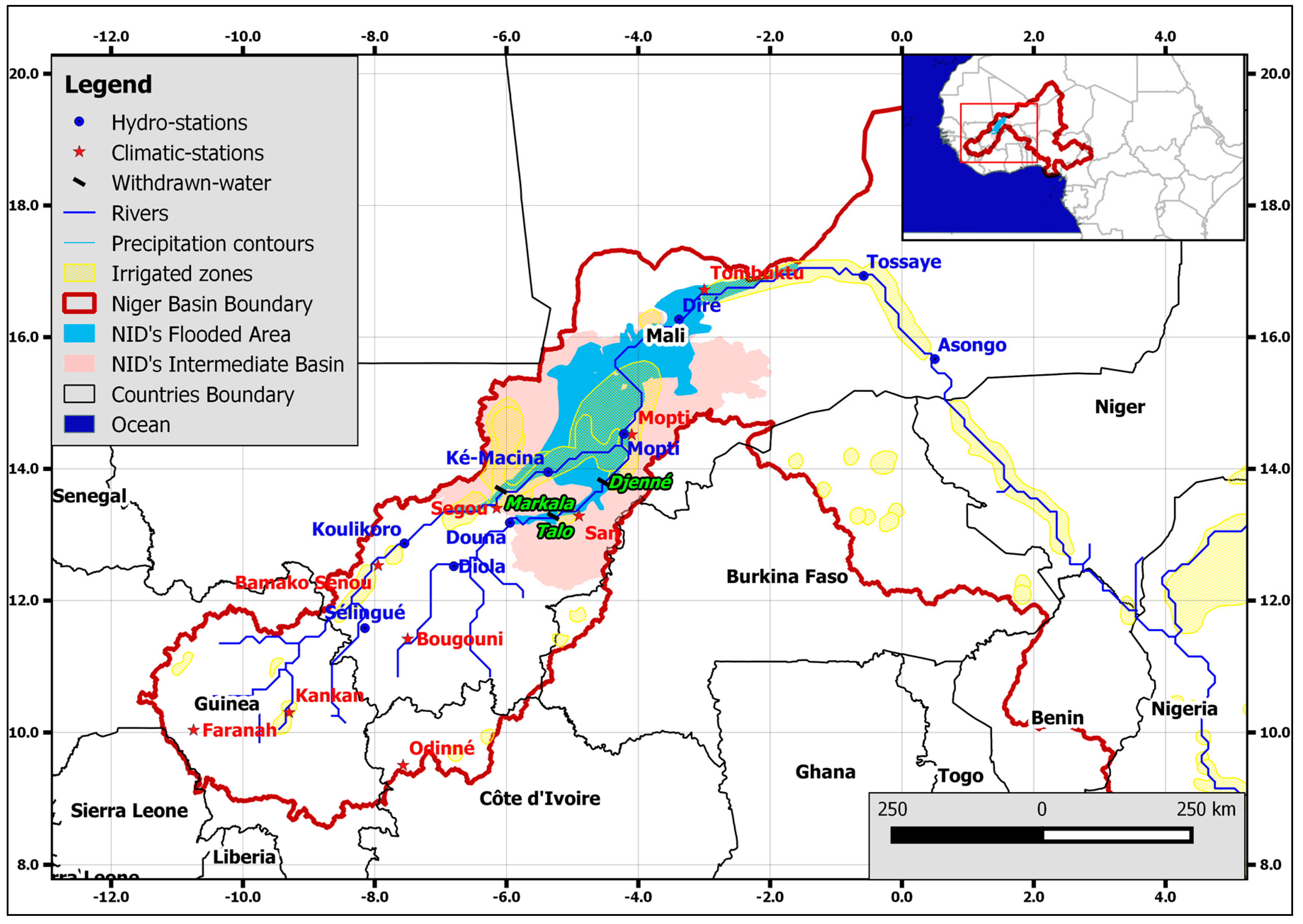
2.1. Study Area

The Niger Inland Delta, located in Mali between the cities of Segou and Tombouctou, spans an area of about 100 km width and 350 km length (Figure 1). The NID receives flow from the Niger and the Bani basins, whose rivers confluence inside the NID near the Mopti discharge station. The NID is extremely flat, and contains many lakes and streams of varying morphology. The altitude of the river bed decreases only by approximately 10 m over the 350 km between the entry and exit of the delta [18].
Flooding in the NID is primarily caused by the annual flood wave arriving from the Guinea part of the Niger River basin [14]. Due to the flood wave, the inundated area of the NID increases and decreases as the flooding varies within the system. The NID, primarily the southern part, functions like a transit plain where the flow is simply delayed, while in the Northern Delta the flooding recharges many lateral depressions and the water is trapped.
Precipitation over the NID is limited to the rainy season from March to October and varies between 350 mm in the north and 700 mm in the south [5]. The rainy season peaks between July and October, but since the flood in the NID is generated by rainfall 900 km upstream rather than locally, peak flow values occur between September and December due to propagation lag times.

2.2. Data

2.2.1. Remote Sensing (RS) Data

To analyze the spatial and temporal variations of the floodplain extent, we used optical and microwave remote sensing data (Satellite-borne measurements of the ETM+ sensor on-board of Landsat 7 and the SeaWinds sensor on-board of QuikSCAT). We acquired Landsat 7 8-Day Raw Composite 7 with a spatial resolution of 30 m, with a thermal band with a resolution of 60 m and a panchromatic band with a resolution of 15 m for the period 1999–2009 from the Landsat archives (http://earthexplorer.usgs.gov). For each month between October 1999 and 2009, we selected the most cloud free scenes from the Landsat archive and applied a Brovey pan sharpening algorithm of the I.pansharpen tool (http://grass.osgeo.org/grass70/-manuals/i.pansharpen.html) to achieve the spatial resolution of the spectral bands of 15 m.
Microwave remote sensing data was taken from the SeaWinds scatterometer instrument onboard the QuikSCAT instrument (available from http://podaac.jpl.nasa.gov/QuikSCAT).
SeaWinds is an active radar scatterometer with the primary mission to be able to get high-resolution measurements of near-surface winds over ice-free global oceans (http://podaac.jpl.nasa.gov/QuikSCAT) and was used for climatological studies, weather forecasting, general meteorology, and other applications, including land use classifications [19].
SeaWinds has a spatial resolution of approximately 25 km and has been in operation for more than ten years from 19 June 1999 to 23 November 2009 [19].
We used the 25 × 25 km version, from Jet Propulsion Laboratory (JPL) (http://podaac.jpl.nasa.gov/OceanWind). We reprojected both satellite data sets to UTM 29 (EPSG 32629).
To validate the classification results from the Landsat 7 images we used NDVI maps created from MODIS satellite land cover data MCD12Q1 (Land Cover Type Yearly L3 Global 500 m SIN Grid “MCD12Q1”) [20].

2.2.2. Hydro-Meteorological Data

To analyze the water balance of the NID, we collected historical records of precipitation, temperature, river discharge, wind-speed, relative-humidity (RH), and evaporation. Meteorological data were acquired at two meteorological stations in Mali situated within the NID, close to Segou and Mopti (Figure 1). Daily precipitation data were available for the period 1950 to 2010; daily air temperature, wind speed, and RH for the stations of Segou and Mopti from 1980 to 2010; and monthly pan evaporation for the station of Mopti from 1970 to 2010.
For stations in Mali, daily hydrological records (daily water level and discharge data) for Ké-Macina, Douna, Diré and Mopti were obtained from Mali’s “Direction Nationale de l’Hydraulique” for a 50-year period (the maximum length of records that was made available) from 1960 to 2013.

2.2.3. Field Irrigation Data

There are many irrigation schemes along the Niger River in Mali. While part of the irrigation schemes from “Office-Riz-Mopti (ORM)” are partly traditional irrigation (free flooding & recession flooding). The “Office du Niger (ON)” irrigation scheme (14°18′ N, 5°59′ W) is destined chiefly for small-holder irrigation and cultivation of flooded rice. Irrigation for ON water is drawn from the Niger River at Markala dam and is conveyed by gravity to a hierarchic irrigation network composed of primary, secondary, and tertiary canals. From the tertiary canals, field canals convey water to the rice basins and evacuate it to a drainage network. This gravity-fed scheme is considered highly successful, independent of rainfall and flood performance [1].
Monthly water withdrawals for the period 2000 to 2010 were available for the two major irrigation schemes. The first irrigation scheme covers an area of about 36,000 ha and is supplied by water abstracted from the Bani River at Mopti (responsible Office-Riz-Mopti (ORM). The second irrigation scheme is supplied by water from the Markala dam along the Niger River and has about 100,000 ha of cropland (mostly rice) under irrigation (responsible “Office du Niger” (ON)). At such big irrigation schemes located in the study area, part of the non-consumptive water previously unevaluated over large hydraulic system is drained back to the Niger River [21].

2.3. Methods

2.3.1. Land Cover Mapping and Flooded Areas Assessment

Initially, we carried out a literature review on image classifications employed in NID land cover mapping [1,14,16,22,23]. Of the different methods used, unsupervised classification was by far the most popular [1,17], but with different techniques. With the exception of color composite image analysis, which showed poor performance in previous comparative studies [14,23], we included the supervised classification with different training data from unsupervised classifiers applied in the previous publications [1,16].
We performed supervised classification and unsupervised classification of Landsat 7 and images and to a SeaWinds onboard QuikSCAT data respectively, and compared the results of these two methods. In addition, this study performed the unsupervised classification of Landsat 7 to use its result to help defining the training areas for the supervised classification. To characterize the landscape and to account for these flooded areas extents, we used a both classification methods to identify major land cover classes and flooded areas using a combination of SeaWinds and Landsat 7 images.

Supervised Classification of Landsat 7 Images

Landsat 7 images from 2000 to 2009 were used for classifying land cover using training areas. However, to find homogeneous zones, the distinction of the training areas was done by the help of an unsupervised classification performed with the ISODATA unsupervised algorithm whose results also used as training samples. Thus, the creation of training areas was improved with the help of unsupervised classification, and existing knowledge on land-cover classification features of the area (Land use map for the West Africa version 2000, collected from AGRHYMET (Agronmeteorology and Operational Hydrology and Their Applications) regional center [24]). Finally, we classified the image mosaic with Maximum Likelihood (ML) and sequential maximum a posteriori (SMAP) algorithm and estimated thresholds and kappa values to distinguish between vegetation and water. The highest Kappa accuracy of 80.37% and 64.36% was achieved from all seven bands both SMAP and ML classifications algorithm respectively.

SeaWinds Classification

SeaWinds data is not typically used to classify land cover but several methods were published for land cover mapping from SeaWinds data [25,26]. In this paper, we compare the results of the classification with the results of supervised and unsupervised classification of Landsat 7 images and by using the MODIS NDVI datasets for the same time period.
To distinguish flooded and non-flooded areas using the SeaWinds data for each month between January 2000 and December 2009, we performed an unsupervised classification with the “I.maxlik” module of the GRASS toolbox and defined the thresholds by comparing the classification results with the maps created using the Landsat classification.

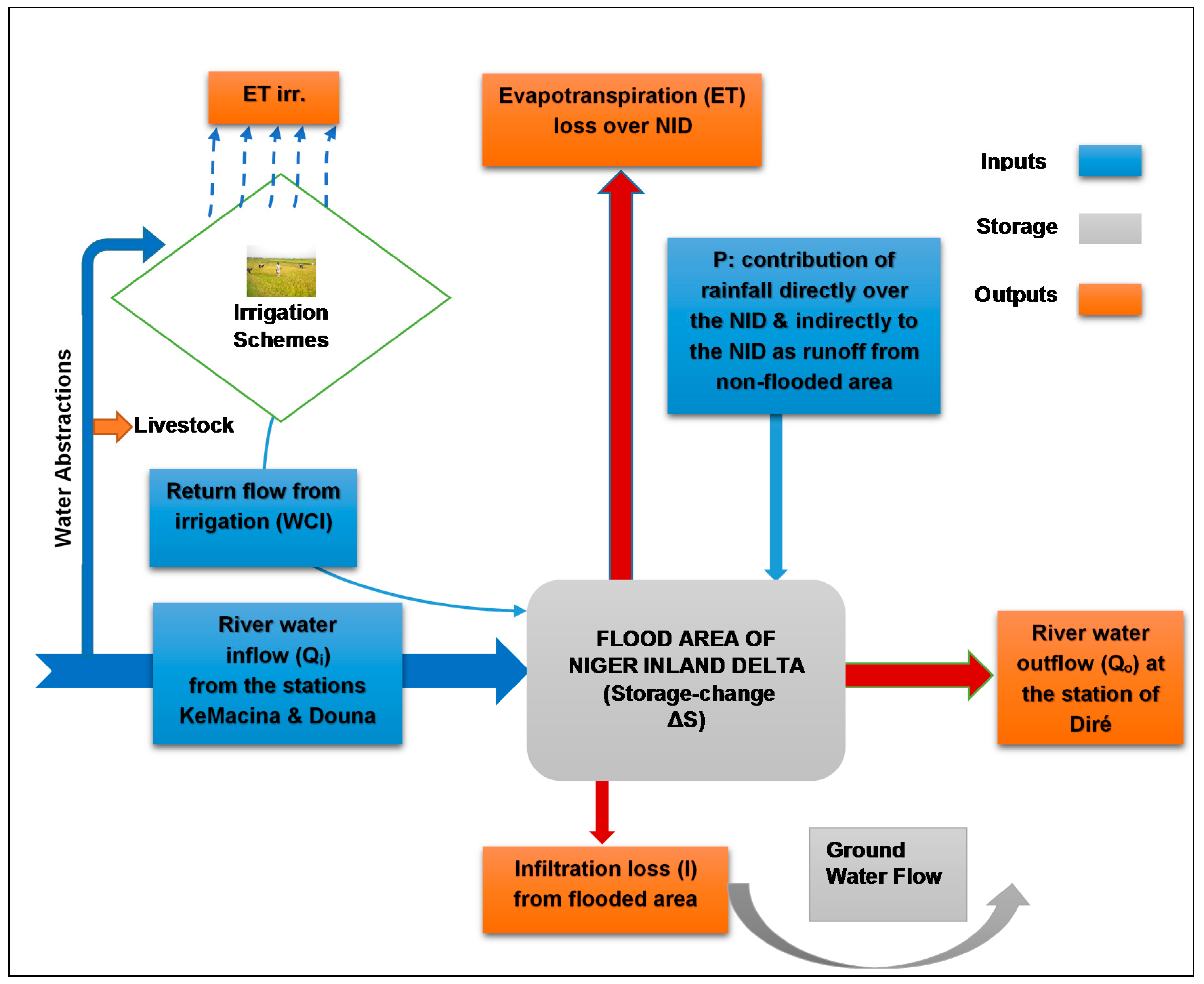
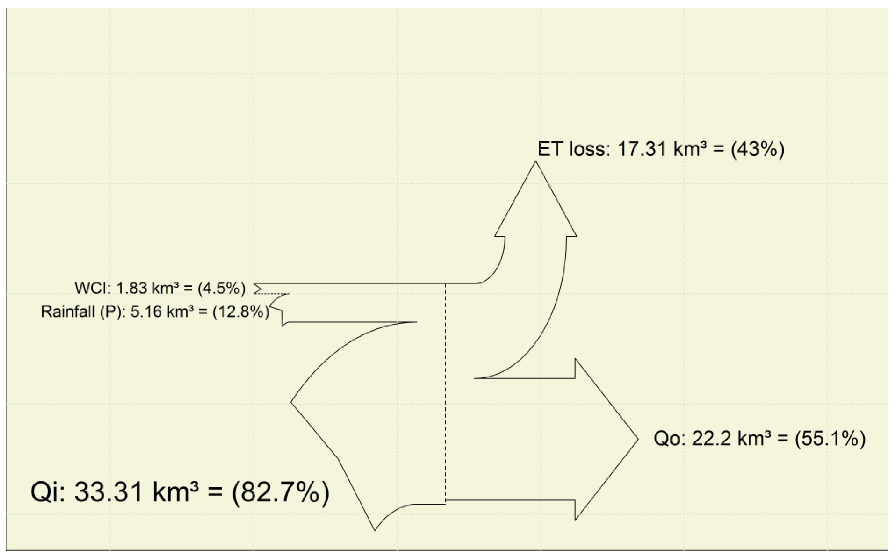
2.3.2. Water Balance of the NID

We conceptualized the hydrological system of the NID as a set of storage terms, and inflow and outflow terms (Figure 2).
The surface water inflow component into the NID is a combination of the discharge records from all major catchments in the upstream basins of the Niger and Bani rivers, as shown in Figure 1, and surface runoff generated within the NID and rainfall over the flooded areas.
The water balance of the NID can be expressed as:
Δ S = Q i ( t ) + P ( t ) ET ( t ) I ( t ) + WCI ( t ) Q o ( t )
where:
  • Δ S = change of storage,
  • Qi = river water inflow, calculated as the sum of discharge measured at the stations KeMacina and Douna,
  • P = Rainfall contribution (directly on the flooded area and indirectly as runoff from areas in the NID’s catchment that drain to the flooded areas),
  • ET = evapotranspiration loss over the NID,
  • I = infiltration loss from flooded area,
  • WCI = return flow from irrigation to the NID’s water balance,
  • Qo = river water outflow at the station of Diré, and,
  • t = time.
  • All units are in (km3·month−1).
Although there is some evidence of groundwater movement in parts of the wetland, there is a highly impermeable clay layer under much of the system [12] which minimizes the influences of infiltration loss. We therefore did not consider infiltration.

2.3.3. Estimation of Water Balance Terms

Evaporation (ET) Loss Computation

Radiation is the principal weather parameters that determines evapotranspiration in the tropics [27]. We tested eight different methods to calculate PET (potential evapotranspiration) models (see Supplementary Information in Tables S1 and S2) that differ with respect to complexity and input data requirements.
We computed PET for each of those methods for the climate data available for the station Mopti and compared those results with measured Class A pan evaporation at Mopti, that was obtained from the “Division de la Climatologie” at the “Bureau Alerte Précoce, Agence Nationale de la Météo” in Bamako, Mali. We multiplied pan observations with a pan coefficient of 0.75, the mean of reported pan coefficients in the Sahel that typically range from 0.70 to 0.80 [28]. Monthly values of ET losses in the NID were calculated by multiplying the remotely sensed area with the calculated PET depth.

Precipitation (P) Contribution to the NID

We interpolated average areal precipitation [29] with the Thiessen polygon method and calculated the direct monthly contribution of precipitation over the remotely sensed are and for the non-flooded areas draining to the NID assuming a runoff coefficient of 5% [5].

Return Flow from Irrigated Fields (WCI)

To estimate the amount of water returning to the NID from irrigated areas as return flow, we subtracted estimated consumptive water use in irrigation schemes from the reported water abstraction data from the Bani and Niger rivers. Consumptive use was calculated as potential crop evapotranspiration, ETirr, by multiplying a crop coefficient, kc with the reference potential evapotranspiration (ET0) computed with the Penman-Monteith equation according to FAO [30].
Net Irrigation water requirement is expressed as (derived from Allen et al. [30]):
I net = ET irr + S + I n P e
where:
  • I net = net irrigation water requirement,
  • ET irr = water requirement ( ET irr = K c × ET 0 ),
  • S = depth of water for soil condition (data collected from the “Office du Niger”),
  • I n = Infiltration rate (refers to percolation losses) within the irrigation scheme (Data collected at “Office du Niger); and,
  • P e = effective rainfall ( P e = P × e r , with P as rainfall over the area and e r as coefficient for effective rainfall).
Gross water requirement (consumptive water use (CW)):
CW = I gross = I net / e p
where: e p is the irrigation scheme efficiency coefficient (0.65, this efficiency is not already considered in the percolation losses), taken from available “Office du Niger” statistics.

Change of Storage (∆S) Assessment

Data surface water level (h) collected from the National Hydraulic Headquarters of Mali, were used for assessment of the storage changes in the NID.
Δ S = A ¯ f × Δ h ¯
  • A ¯ f = Average flooded area (km2) between two time intervals,
  • Δ h ¯ = average variation of surface water level (in km) between two time intervals, calculated from the mean water height at the gauging stations (Mopti, Diré & Ké-Macina) between two time intervals.

2.3.4. Analyzing the Water Balance

The closing of the water balance over the NID (NIDWat) at monthly time steps was carried out in two steps. First, we assessed the water budget terms over the NID described above independently of the terms of the water balance equation (Equation (1)) using input datasets derived from the observed and satellite data time series. Then, simulated water losses were compared to discharge differences obtained from the inflow-outflow for annual time steps.

3. Results

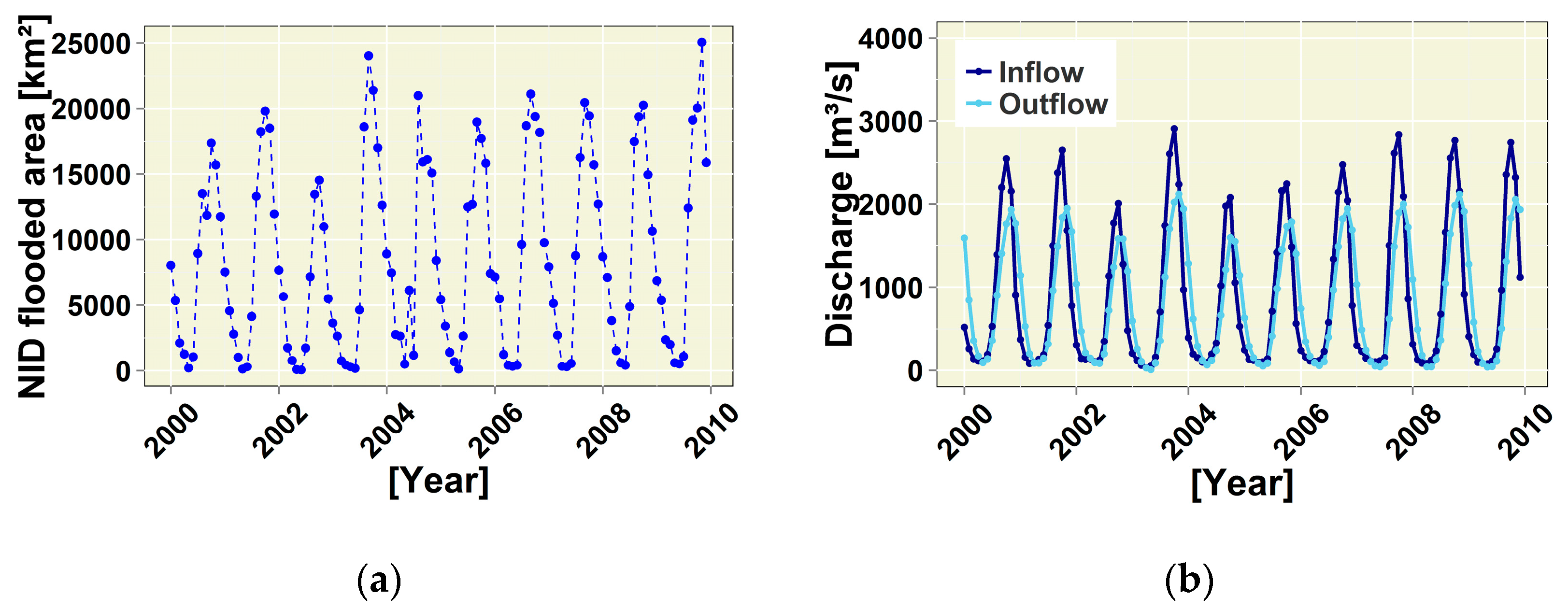
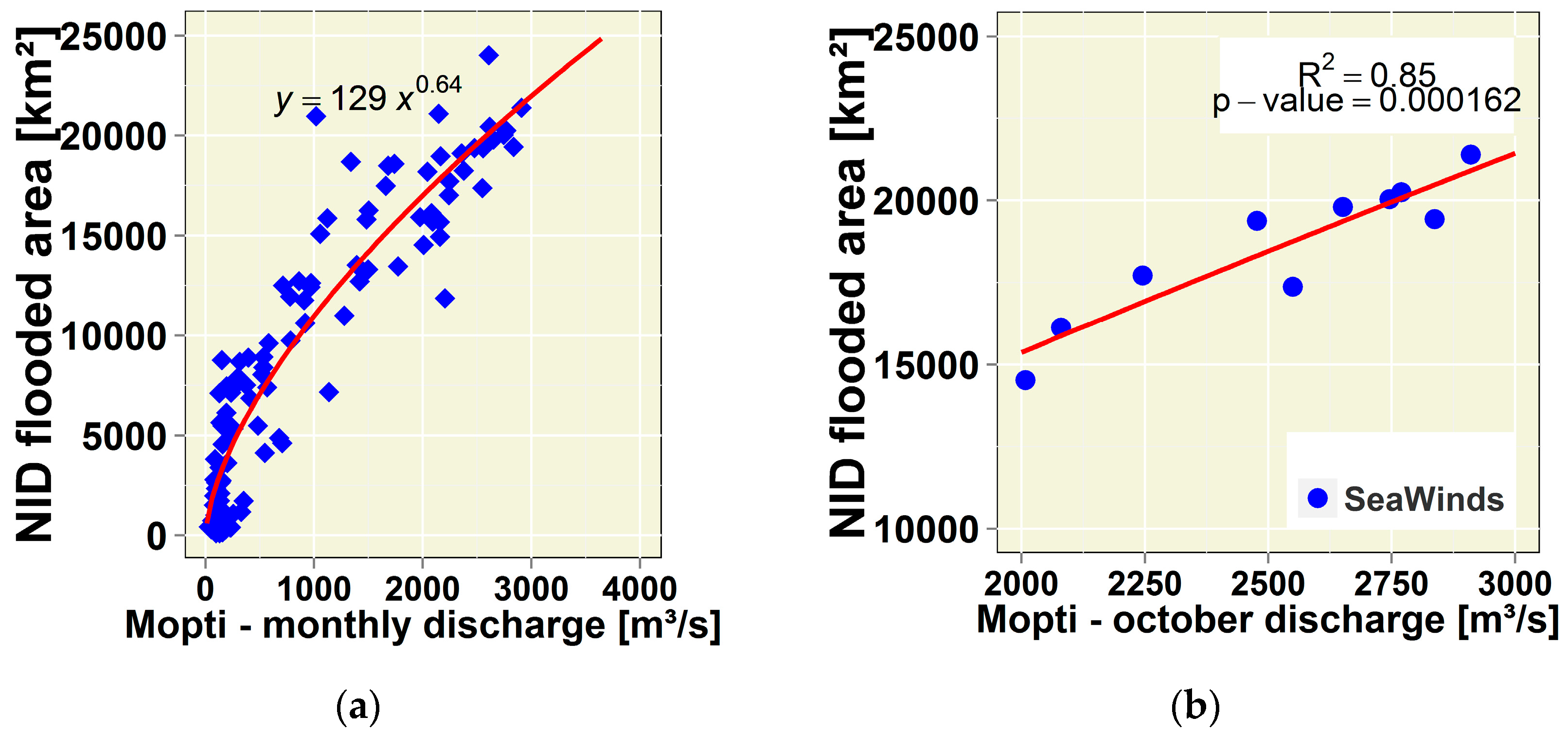
3.1. Assessment of Flooded Area

The maximum monthly flooded surface area in the NID obtained from SeaWinds data varies between a maximum of 25,054 km2 in 2009, and a minimum of 14,525 km2 in 2002 (Figure 3a). The 2000 to 2009 mean of the maximum flooded surface area was 14,977 km2 with a standard deviation of 7227 km2, highlighting the significant inter-annual variability. During the dry season, the flooded surface area receded progressively to a minimum of 317 km2 (2000 to 2009 inter-annual mean) then following April, they increased in June and rose rapidly in August. Minimum values, measured between March and April, vary between 300 km2 and 4000 km2.

Remotely Sensed Flooded Area Comparison-Discharge and Area Relationship

Following other studies [1,16,31], we analyzed the relationship between the maximum discharge at Mopti and the extent of the flooded area in the NID. This relationship can best be expressed by a non-linear regression model:
A f = 129 × ( Q i ) 0.64
( R 2 = 0.92 )
where: A f is the flooded area in km2; and Q i is the mean monthly inflow data in m3s−1 at the Mopti gauging station (Figure 4a).
This relationship between inflow and flooded area is plotted in Figure 4a for the last 10 years; implying that the behavior as the flood rises in Figure 4b led to a greater surface area during maximum October flow discharge at Mopti. The positive slope of the regression line in Figure 4b indicates a positive relationship between the maximum inflow discharge and the peak flood extent.

3.2. Water Balance Hydrological Variables Estimations

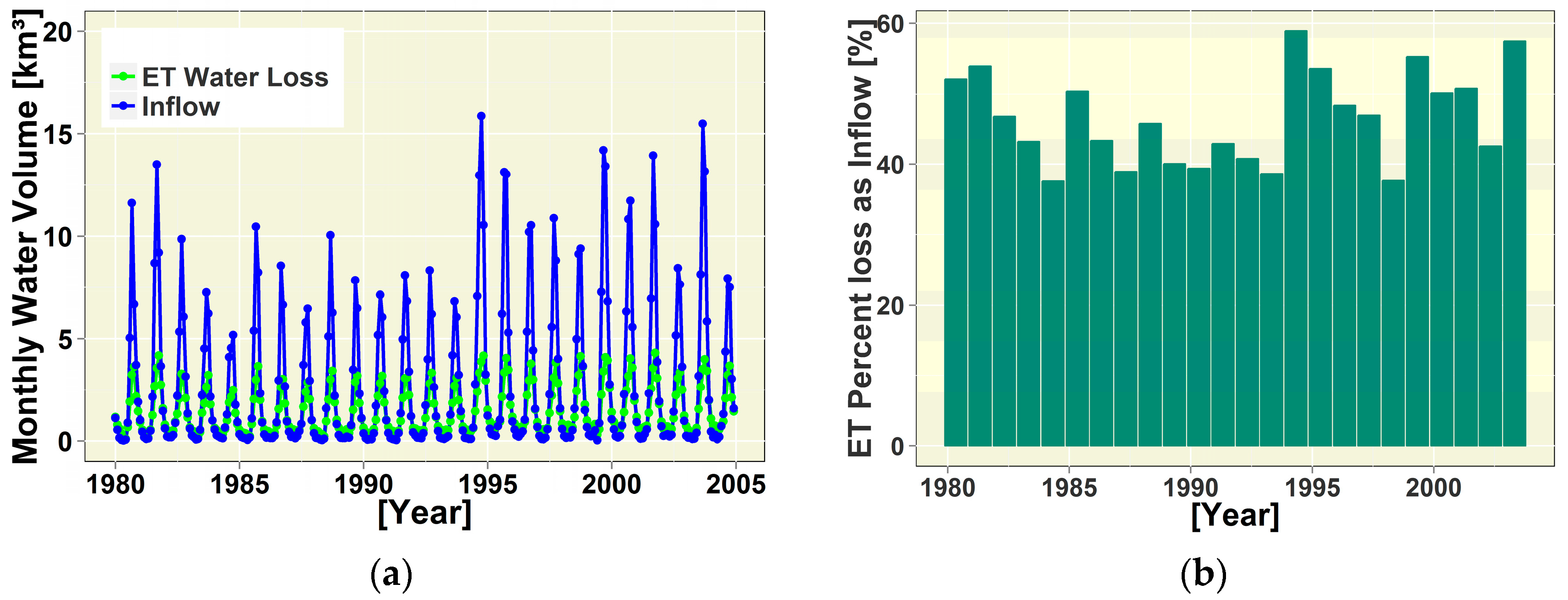
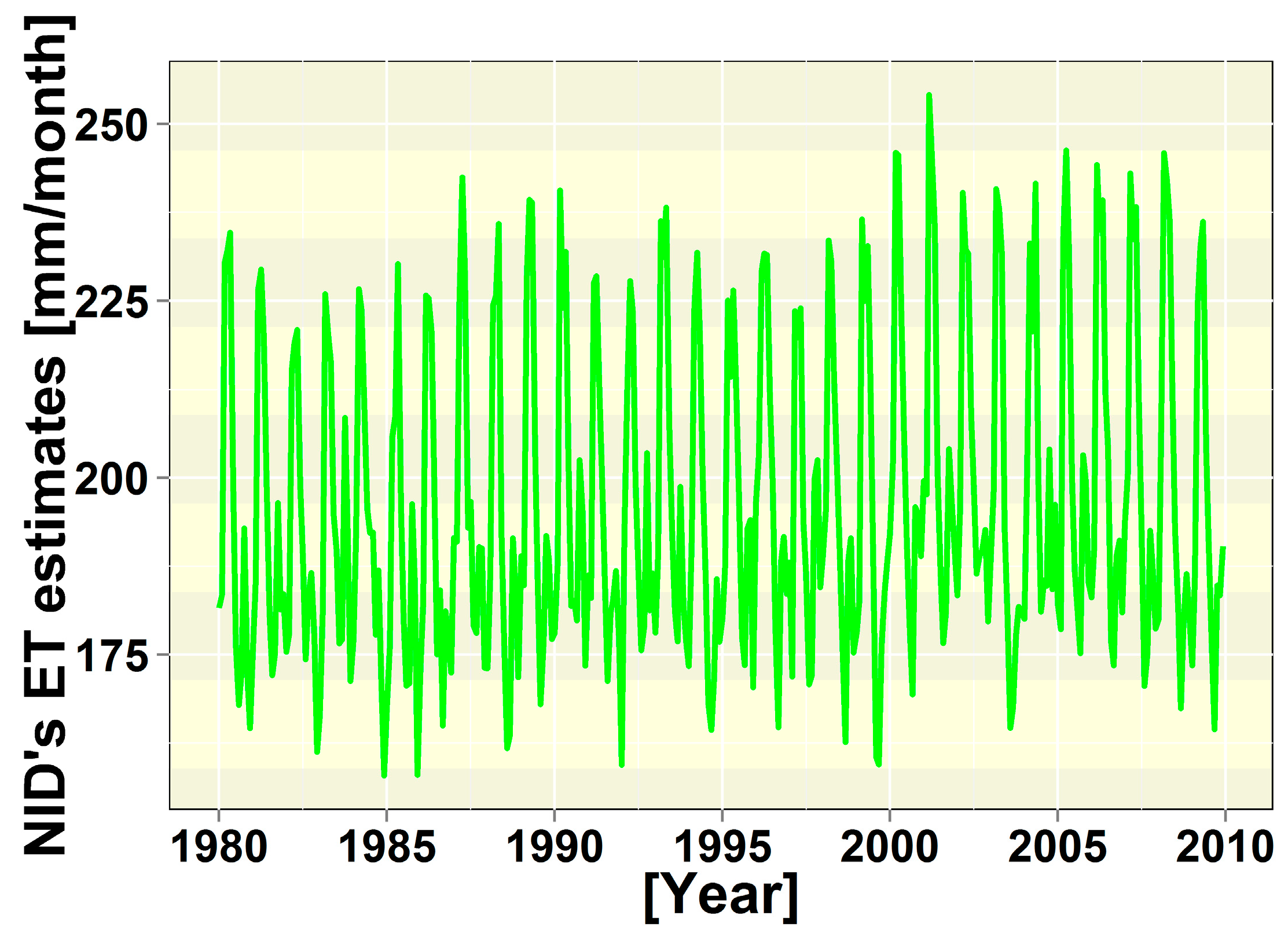
3.2.1. Water Losses (Evaporation (ET)) Estimations over the NID

Comparing the results from the eight PET models with the Mopti class A pan records over 360 months (January 1980 to December 2009), we found that the modeled data adequately represented the dynamics observed. The simulated mean annual evapotranspiration rate computed using the eight PET models showed significant differences ranging from −500 to 500 mm per year. Comparing the recorded pan evaporation data at Mopti and using performance criteria recommended by Moriasi & Arnold [32], we found that the Penman-Monteith model is best suited to calculate PET in the NID. The comparisons of the methods are first made on an annual basis. The observed yearly evapotranspiration and the relative errors of the calculated evapotranspiration to the observed pan values are presented in Table 1. It is seen that on a mean annual basis the Modified Turc model (2549 mm) gives the smallest error & the lowest bias compared with measured pan evaporation (2558 mm), followed by the Hamon (2409 mm), and Penman-Monteith (2370 mm) models.
Regarding the Pearson coefficient of correlation, it is seen that the PMO (Penman-Monteith) model and the Priestley-Taylor model have the highest coefficient’s values, with r = 0.73 and r = 0.72, respectively. The Modified Turc method has the lowest value, with r = 0.01 as shown in Table 1.
The calculated water loss due to evapotranspiration is shown in Figure 5. The percentage of ET loss calculated for each annual inflow in selected hydrological years (Figure 6b) was compared with corresponding available discharge data inflow (KeMacina + Douna). Time series of input water volumes in the Niger Inland delta and of the water losses through the NID show that the average percentage of water losses, due to the high evapotranspiration, is approximately 50% (Figure 6b). Observations reveal that the Niger River at NID experienced a downward shift in discharge in 1982 and 1992 is proportional to the decrease in ET loss; and is also coherent as observed rise from 1994 till 2004 (Figure 6a). However, a large volume of inflow in the NID at Mopti led to greater floods in the area and hence larger ET loss (Figure 6b).

3.2.2. Accounting for Rainfall and Estimating Return Flow from Irrigation

The annual total contribution of precipitation & runoff over the wetland, calculated from the observed average rainfall data over the estimated flooded areas and runoff from non-flooded areas draining to the NID, varies between 3.10 and 9.12 km3. Precipitation draining to the NID from non-flooded areas is around 2.6 km3 per year indicating a non-negligible contribution to the overall water balance of the wetland.
The volume of the abstracted water needed for irrigation based on the available irrigation details from the ON amounts to 0.223 km3 per month. “Office du Niger” takes approximately 2.5 km3 water per year; this becomes more important, when irrigating more areas. For the “Office Riz Mopti” (ORM) we consider data on the Bani River only. Before the Bani enters the Niger Inland Delta, 0.291 km3 per month (Table 2) is taken for irrigation at Djenné and Talo dams. This represent an average flow reduction from Bani River to the NID expected at Mopti (Table 3).

4. Discussion

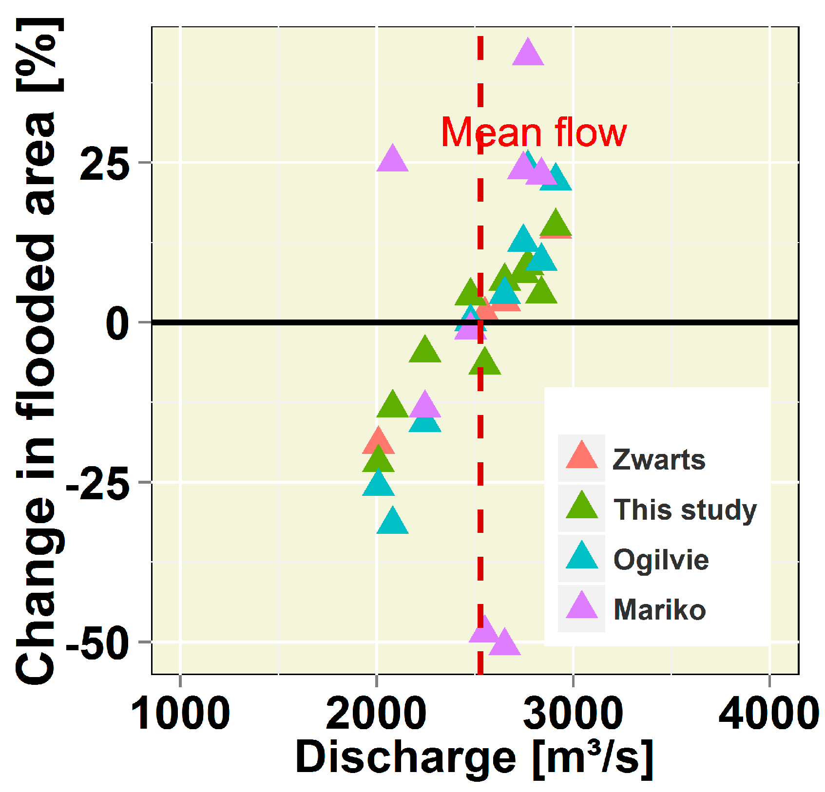
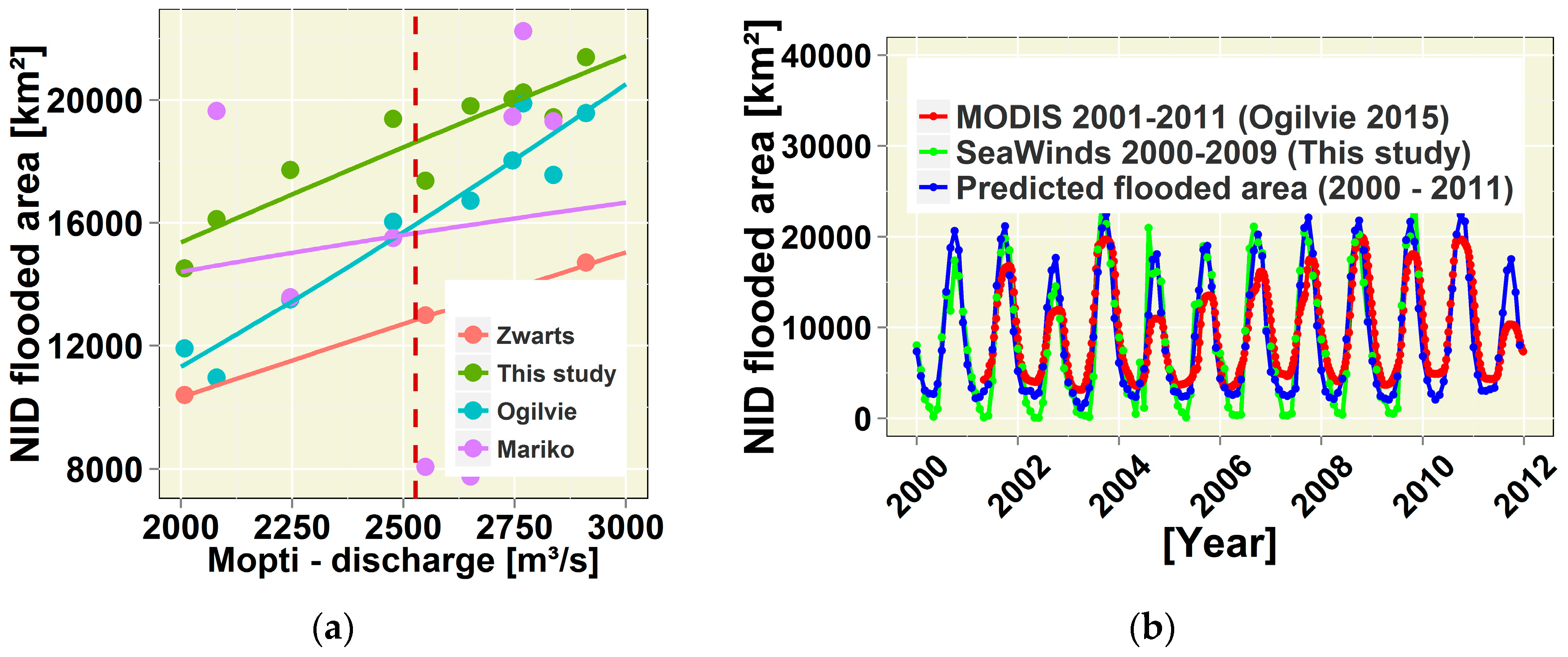
4.1. Comparing Remotely Sensed Flooded Areas with Previous Estimates

Estimates of the flooded area in the NID using remotely sensed data were carried out by a number of studies [1,16,31]. Generally, our estimates of the monthly extent compare well with these studies (Figure 7b). This is an important result, as all previous studies were optical based and therefore limited by clouds during the flood rise (Figure 7a). However, the first impression shows that the SeaWinds classification results in higher wetland area extents than the Landsat 7 classification, when considering all 77 scenes, where the Landsat images as well as the SeaWinds images are available.
This high difference is to be expected for two reasons. First, the grid size of the SeaWinds raster has an average area of 3014.3 km2 per pixel, while Landsat 7 has a pixel size of 225 m2. Secondly, SeaWinds reacts much more sensibly to the availability of moisture, while Landsat 7 is more sensitive to vegetation growth, at least in the bands five and seven, and the vegetation needs some reaction time to the change between drought and abundance of water. Also, by analyzing the created SeaWinds time series no dominant trend is recognizable. The main reason for this could either be the short time span of the observation or just because no real general shift exists. Comparing the dry season and the rainy season separately, no further evidence of extern influence like through the global climate change can be found. Only the maximum spread of the wetland seems to have a weak tendency to an increasing value, as visible in the Figure 7a.
The Mopti gauging station is usually used to model the annual floods in the NID [1,5], as its central location allows study of flow variations in both the Niger river and, indirectly, the Bani River, a major tributary. Changes in rainfall in the Niger and Bani upper catchments are known to be main drivers of fluctuations in the total flooded area [5]. The annual flood dynamic observed through remote sensing is consistent with the NID flow regime (Figure 3b), providing a correct representation of the flooding. Interannual variations in the max flooded areas are also strongly correlated (about R2 = 0.90), with the maximum monthly flows in October at Mopti, suggesting a strong dependence of the area on the peak amplitude of the flooding. The range of values obtained and their variation according to peak flow in October are consistent with previous remotely sensed estimates [1,16,31]. The difference in estimates by different methods used for the remote sensing area estimates reveals the difficulties in assessing the spatio-temporal dynamic of the flood area extent. Mariko [31] was limited in his study with the number of suitable images of NOAA AVHRR products to characterize the flooded area relationship with discharge. Zwarts et al. [1] used 24 Landsat images spread over several years to derive a correlation between flooded areas and the Akka stage level. Ogilvie et al. [16] used MODIS images and was limited in the accuracy in determining the rise of the flood due to the presence of clouds. Our area estimates based on SeaWinds demonstrate the potential of radar remote sensing to overcome these limitations.
The predicted extent based on Mopti discharge which is the annual flood dynamic observed through nonlinear model, appeared coherent with MODIS’s estimates by Ogilvie et al. [16] (Figure 7b); providing confirmation of the method’s ability to correctly represent the variation of the flood. Therefore, the flooded surface area extent in the previous years could be predicted and, this partly explains the variation along the non-linear regression line shown in Figure 4a. However, the microwave remote sensing data based on which the nonlinear model was established, overestimates the minimum flood extent area (Figure 7b). This is in line with the explanation by Aich et al. [33] and Liersch et al. [34] with regards to the substantial uncertainty on the surface flooded area modeling in the NID. The reason they mention it is likely the effects of land use changes, and lack of detailed regional studies in this regards for the NRB. Besides, observed increasing discharge since 1994 in Mopti and Douna increases the flooding extent and in combination with increasing population pressure led to greater irrigation water use in the study area. This is in contrast with the observations of Ogilvie et al. [16] who reported that in 2004, the peak flooded area in the NID was 45% lower than in 2008. Still, between 2004 and 2009, a non-linear decline in this area is recognizable
Furthermore, the most recent decade (2000–2009) display higher flooded area compared to decades 1990s and 2000s. Figure 8 illustrated the 2000–2009 of relative mean area change at NID over sample period of our analysis of maximum in the extent of flood with maximum peak flow. Observed percentage change in flooded area trends highlights slightly its response with increase in flow (Figure 8). The flooded area change witnessed in the NID is attributed in general to changes in peak flows, and in particular to land use or irrigated agriculture; which led to ~10% increase of flood extent from the month of October under the reference period of 2000–2009 (Figure 8). The interpretation of this result is difficult since no local studies are known that confirmed the changes in the October’s flood area extent. However, Zwarts et al. [1] and Orange et al. [3] explained that this result might be an effect of the delay of the high water wave through the Niger Inland Delta which varies between 1 and 2 months.

4.2. Comparing Water Balance Components with the Previous Studies

The average annual rainfall contribution (varying from 3.26 to 8.4 km3/year) to the water budget of the NID is in line with the recent estimated direct precipitation over the wetland by Ogilvie et al. [16] over the MODIS flooded areas which varied between 2.6 km3/year and 8.5 km3/year. Despite neglecting of groundwater in line with previous studies [1,11,16,35], this study uses storage changes and the remaining flows parameters to assess the balance. Our estimate of the rainfall contribution to the NID’s flooded area is fairly similar to the recent calculated water budget residual terms (infiltration (which we neglected) and rainfall runoff) in between −0.7 and 5 km3 [16]. Monthly average NID’s flooded area storage changes of 0.329 km3 was estimated. This is in line with previous studies who suggested that its contribution to the NID floodplain is minimal [5,11,35]. Storage also decreased during the wet season (April–September) and slightly increased during October to March in concordance with seasonal rainfall pattern [1,36].
Regarding the ET component, understanding concerns of local water losses will contribute to the analysis of relevant hydrological processes and improvement of NID’s water budget [16]. ET losses were calculated from remote sensing estimated flooded areas and evapotranspiration data rates across the NID from ET models for 1980 to 2004. Over the period of 1980–2010, monthly potential ET values from north to south ranging between 157 and 255 mm/month, and the mean monthly PET across the NID is estimated at 196 mm/month. This value is slightly higher than previous evaporation estimates of 192 mm/month by Olivry [11] who used the proportionality between flooded areas and total evaporation to assess the flood surface areas variation in the NID. Measuring ET also takes soil moisture and vegetation across the wetland into account, which would increase overall evaporation loss.
Potential ET rates in the NID’s wetland from 1980 to 2009 are 2.61 to 9.56 mm/day, which are slightly higher than the values of 3 to 7 mm/day in Dadson et al. [12]. The annual cumulative ET loss over the entire NID ranges approximately between 12.71 and 21.78 km3, which is 196.3 mm/month (1.443 km3 per month), close to the range of values modelled by recent studies from the period 1980–2002, notably 140 to 240 mm/month in Zwarts et al. [1]. However, evaporation from flooded areas may have been overestimated slightly, as evaporation rates from the NID, for submerged vegetation area, can be less than those of open water (McMahon et al., 2013 as cited by Ogilvie et al. [16]). However, uncertainties from remotely sensed flooded areas are expected to be more determinant with regards to wetland’s evapotranspiration estimates. Though, potential ET is highest during the dry season, total ET from the NID is higher during September, October, and November due to the large surface area flooded. In addition, spatial variations in actual evaporation [12] were significant, due to higher PET values in the northern areas and the longer flood durations along river stretches and lakes.
To enhance the water budget of the NID to distinguish the water availability, it is important to look beyond abstracted water from rivers (Niger and Bani) for irrigation. The return flow which referred to the non-consumptive water used drained to the NID and generated by the irrigation schemes, was computed. The average water volume of return flow from irrigation dataset (Table 3) is ranging from 0.013 km3 to 0.559 km3 per month. This is lower than the values between 2.50 km3 in 1994 to 2.85 km3 in 1999, with an average of 2.69 km3 per year of the total annual intake for irrigation (at ON). It is important to highlight that this is before the KéMacina station, and therefore the abstraction is not relevant in the water balance, it is indeed the WCI which is of interest here, and this totals 1.8 km3. Some of this is from Office Riz Mopti and the total balance of these may be null (as withdrawals, PET and return occur within the NID), hence it’s really the return flow from Office du Niger, which was not previously estimated, and this is in the order of 1.2 km3 per year in line with previous findings [1]. Zwarts et al. [16] also noted the importance of inter-annual variability in irrigation water use impacting on the NID’s flood area extent. Our computed relative average annual return flow from irrigation is lowest (about 4.5%) over the NID, but significant for the water balance and on downstream wetland benefits (Figure 9). The range of values obtained were consistent with previous value of 3.7 km3 estimated by Zwarts et al. [1] (less than 10% of total inflow) of annual water intake for irrigation, though the value was moderately superior and met our expectation.
NID’s floodplains are being modified as the result of water management activities, in particular large-scale irrigation schemes; which, irrigation water increases with higher crop evapotranspiration and high intake of water abstracted from rivers (Niger & Bani) can be explained due to a lack of an adequate efficient irrigation system [1,15,37]. Some studies were conducted, since the early developments of the “Office du Niger” and have confirmed this hypothesis. The level of the water table is increasing after many years under the influence of irrigation in areas of “Office du Niger”, this rise is linked not only to the return of irrigation water in delta, but also to the permanent retention of water in irrigation channels [38]. With use of surface water for irrigation, e.g., in large River valleys, drainage and net groundwater recharge may have increased [39]. Our analysis suggests that the return flow from irrigation can only partially replace the lost water abstracted from reducing floodplain inundation. Thus, further extension of irrigation schemes within the rivers basin should also be avoided, because of the expanding demand for irrigation which will increase the water losses.

4.3. Water Balance (NIDWat) Analysis

The water balance cannot be closed by the data available. Figure 9 shows the Sankey diagram of the water budget over the NID’s surface flooded area which shows an error of 1.9%. Our simulated mean annual evaporation loss of 17.31 km3 is superior to that of the discharge differences (11.18 km3). The average of evaporation losses is in accordance with the previous result based on the hydrological balance.
The water balance was performed from observed hydro-climatic and optical & microwave remote sensing data adapted from the NIDWat modelling approach providing input and output fluxes across the NID’s wetland (Figure 9). This NIDWat model also provides the main features that leads to the explanation of the overall hydrological functioning of NID’s reservoir. However, NIDWat in the present situation differed on approaches compared to models of above mentioned publications in which the natural variations as well as the impact of human activities (e.g., irrigation aspect) on NID’s floodplain are not well captured. Hence, for this article, the output of NIDWat is mostly compared with the recent model results by Ogilvie et al. [16], as mentioned in the introduction of this paper because the two approaches can be used in a complementary manner.
The calculated amount of water reduction in discharge difference (inflow minus outflow) for the inlet and outlet gauging stations is compared with the results of NIDWat. The annual mean evapotranspiration’s are overestimated as compared to the discharge differences between inflow and outflow over the NID, which is confirmed by Ogilvie et al.’s [16] results. This implies that other hydrological component over the wetland must be accounted for; and also, the actual ET losses would be considered. Our simulated mean annual evaporation loss of 17.31 km3 (i.e., 43% of the total input) was found consistent with a mean value of 17.2 km3 in Ogilvie et al. [16]; and moderately superior to a value of 11. 4 km3 (i.e., 33%) in Zwarts et al. [1]. Values for the contribution of rainfall, and values on the return of water withdrawal for irrigation are found coherent with the references mentioned above. The water budget’s difference is 1.9% between the input fluxes and output fluxes confirms that our model provides an adequate representation of the potential evaporation losses (Figure 9). The interpretation of this error is difficult since no local studies are known that confirmed the water budget modeled in the present study. However, Ogilvie et al. [16] assumed that his water budget residual term corresponds the difference between infiltration and runoff generated by rainfall falling upon non-flooded areas of the NID. Hence, the good performance of the NIDWat model confirms that, SeaWinds data and the WCI estimates may therefore be used to provide additional insights and refine the water balance of the NID. Nonetheless, the trends generally remain good, even if some parameters are not considered; the limitations with respect to data availability and uncertainties in the significance of the estimated parameters, however, remain.

4.4. Uncertainty and Outlook

Input data used in the estimates of the available energy for ET are source of uncertainty since measured solar radiation is not available at meteorological stations in or near the study area. In addition, we used only Mopti pan recorded data pan for the whole study area due to the lack of other local pan recordings for our study area based on the assumption that the climate classification is the same [40]. The uncertainty of the single ET models in percentage deviation from the mean ET of 17.67 km3/year is in the range of −15.31% to +15.54%. PMO has the smallest differences to this mean value (−2%) resulting in a water balance error of 0.79 km3/year. The water balance error is calculated by summing all in and outflows. The uncertainty in ET results in a water balance error in the range of −2.31 to +3.14 km3/year. This error is the smallest (0.435 km3/year) when the ET losses are calculated as the mean over the eight models is used and only slightly higher when the PMO model is applied.
Our water balance modeling approach, like previous studies to assess water losses under hydro-climatic conditions [1,11,16,31] is limited by some assumptions and some processes that are not represented in the model. One of these limitations is the neglect of infiltration from flooded areas and rainfall. Although infiltration is the dominant process of groundwater movement in portions of the wetland [5]; and could become more important in a water balance. Therefore, infiltration process in NID’s wetland can potentially lead to the error in balancing the water fluxes over the NID. Constraints in our water balance are not only caused by constraints in the characterization of hydrological processes but also by uncertainties arising from the data.
Moreover, the possible changes in the NID hydraulic pathways due to dams or land use changes as discussed in Ogilvie et al. [16] were not considered.

5. Conclusions

This study demonstrates how remote sensing data can be used to help conducting hydrological process analysis at high temporal and spatial resolution across large wetlands. Understanding surface flooded area processes for the Niger Inland Delta are crucial for water balance purposes. The advantage of effectively mapping wetland using microwave SeaWinds data have been illustrated and allows describing the flooding dynamic in the delta in terms of inundation extent. We have shown a clear correlation between maximum October flow at Mopti and peak flooded area in NID. The results are in good agreements between the estimated flooded area data and the remotely observed surface flooded area from past studies.
We present the Penman Monteith model as best in representing the potential ET in our study area. In addition, this study shows how knowledge from the flood characteristics was used to significantly improve our understanding of hydrological processes in the NID’s floodplains and their interaction with hydrological observations. Thus, NIDWat was developed to understand the hydrological functioning at play in NID’s flooded area. Estimated flooded areas were used to refine evaporation estimates as well as precipitation over the wetland. Additionally, actions from irrigation schemes on a large scale (e.g., ON & ORM) have implications for water balance in the system. Despite often neglected infiltration and ground water fluxes, annual differences in annual rainfall, discharge and evaporation over the wetland are essential to explain inter-annual variations in the water balance. The water balance model NIDWat was shown to be suited for assessing the hydrologic characteristics of NID’s wetland. Its information can be used into existing hydrological models on the basin to improve runoff simulation downstream the NID.

Supplementary Materials

The following are available online https://www.mdpi.com/2306-5338/4/3/40/s1, Table S1: Data availability and periods of records for the main climatic variables and evaporation at Mopti synoptic station (longitude = −4.1, latitude = 14.52, Elevation = 272 m); Table S2: Inputs data of all potential ET methods used in this study.

Acknowledgments

This study was funded by the German Ministry of Education and Research (BMBF) through the West African Science Service Center on Climate Change and Adapted Land Use (WASCAL; www.wascal.org), that supports the Graduate Research Program Climate Change and Water Resources at the University of Abomey Calavi). We thank AGHRYMET regional center, Niger Basin Authority, and Niger & Mali Meteorological and Hydrological Service for providing the hydro-meteorological data for the Niger Basin.

Author Contributions

Moussa Ibrahim, Dominik Wisser, Abdou Ali, Bernd Diekkrüger, and Abel A. Afouda conceived the study, developed the methodology. Moussa Ibrahim performed the field work, collected the data, and conducted the analysis with Dominik Wisser and Abdou Ali. Manuscript was drafted by Moussa Ibrahim, with input from Dominik Wisser, Ali Abdou, Ousmane Seidou, and Adama Mariko; while Abel A. Afouda and Bernd Diekkrüger supervised this part of the work.

Conflicts of Interest

The authors declare no conflict of interest.

Abbreviations

The following abbreviations are used in this manuscript:
ABTSimple Abtew equation
AGRHYMETAgrometeorology and Operational Hydrology and Their Applications
CWConsumptive Water used
DEMDigital Elevation Models
HAMHamon evaporation model
HARGHargreaves evapotranspiration model
JULESJoint UK Land-Environment Simulator
MAKModified Makkink equation
NIDNiger Inland Delta
NIDWatNiger Inland Delta Water balance model
NRBNiger River Basin
ON“Office du Niger”
ORM“Office Riz Mopti”
OUDOudin evapotranspiration model
PETPotential Evapotranspiration
PMOPenman-Monteith combination equation
PRTPriestley-Taylor method
RMSERoot Mean Square Error
RSRRatio of RMSE to the standard deviation of the observations
TURModified Turc evapotranspiration method
WASCALWest African Science Service Center on Climate Change and Adapted Land Use
WUWithdrawn water
WCIReturn flow from irrigated fields
ZEFCenter for Development Research

Appendix A

Appendix A.1. Potential PET Estimation Methods

(1) Edited Potential Evapotranspiration (PE) Model Published by Oudin et al. [40]
PE = R e Δ ρ   T a + 5 100   if T a + 5 > 0
PE = 0
where:
  • PE = rate of potential evapotranspiration in mm per day;
  • Re = extraterrestrial radiation in MJ per m2 per day;
  • λ = latent heat flux for the vaporization (as 2.45 MJ per kg);
  • ρ = density of water (ρ = 995.6502 kg per m3); and
  • Ta = air temperature (°C) which correspond to the mean daily air temperature.
(2) Penman-Monteith Combination Equation (PMO)
The Penman-Monteith equation is the most physically based model and corresponds to the Penman equation which is the updated equation recommended by FAO [41] known as the FAO-56 Penman-Monteith. It is expressed as [30].
PMO = 1 λ   Δ ( R n + G ) + ρ a c p ( θ s θ ) Δ + γ ( 1 + r s r a )
where PMO is the ET rate (mm d−1), Ta is mean air temperature (°C), v is wind speed (m s−1) at 2 m above the ground, G is the soil heat flux, which can usually be neglected in the tropics [41], Δ is the slope of the saturation vapor pressure curve, γ is the psychrometric constant (see calculation under radiation), θ and θ s is the actual and saturated vapor pressure at given RH in kPa (see calculation under radiation), ρa is the mean air density at constant pressure in kg m−3, cp is the specific heat of the air in MJ kg−1 °C pressure in kPa (see calculation under radiation), rs is the surface resistance in s m−1,and ra is the aerodynamic resistance in s m−1. rs in the case of open water is 0 and ra can be calculated from Thom and Oliver (1977) (as cited in Schwerdtfeger et al., [17]):
r a = 4.72 ( ln ( 2 z 0 ) ) 1 + 0.54   v
where z0 is the roughness length, which can be set to z0 = 1.37 mm [41].
(3) Priestley-Taylor Equation (PRT)
Xu & Singh [42], highlighted that the Priestley-Taylor model derived after Priestley and Taylor, (1972); is a simplified version of the combination equation of Penman (1948). It is generally used when surface areas are wet. Thus, the Priestley-Taylor coefficient α PRT is introduced, which is multiplied by the energy component:
PRT = α PRT Δ Δ + γ R n λ
where α PRT can be set to 1.18 [17].
(4) Hargreaves Equation (HAG)
The combined form of Hargreaves equation (HAG) is the Hargreaves and Samni (1982, 1985) formula after Hargreaves, 1975 (as in Schwerdtfeger et al. [17]). The equation can be expressed as:
HAG = 0.0135 ( T a + 17.8 ) R s
where: T a is the average temperature, R s is the global solar radiation which can be calculated from formula for estimating R s from the temperature range ( TR ), the extraterrestrial radiation ( R a ); and an empirical coefficient ( k r ) depending on the station location: R s = k r × R a × TR 0.5 .
(5) Modified Makkink Equation (MAK)
Makkink (1957) estimated ET in millimeters per day over 10-day periods for grassed lands under cool climatic conditions of the Netherlands. After Makkink, 1957; Abtew and Melesse, 2013 (as cited in Schwerdtfeger et al. [17]), calibrated the Makkink equation to the simple Abtew method (Equation A6) for tropical South Florida and has the following form:
MAK = 0.743 Δ S t ( Δ + γ ) λ
where: S t is the solar radiation in MJ m−2 day−1 (see Equation A23 below).
(6) Simple Abtew Equation (ABT)
The simple Abtew equation was developed for tropical South Florida by Abtew and Melesse, (2013) from open water evaporation and wetland lysimeter studies (work cited in Schwerdtfeger et al. [17]). It can be expressed as:
ABT = K 1 S t λ
where: K 1 is a dimensionless coefficient given with 0.53 [17].
(7) Modified Turc Equation (TUR)
We use the empirical Turc equation modified for a humid subtropical region. Tmax is used instead of Ta since it showed a better fit with observed data [17]. The modified Turc equation is written as:
TUR = K 2 ( 23.89 S t   +   50 ) T max T max + 15
where the coefficient K 2 has the value 0.013 derived from the original Turc equation by Abtew and Melesse, (2013) (as in Schwerdtfeger et al., [17]).
(8) Hamon Equation (HAM)
Hamon (1961) (as cited in Oudin et al., [40]) derived a potential evapotranspiration method based on the mean air temperature and is expressed as:
HAM = 2 × DL 2 × θ s × e ( T a 16 )
where:
  • HAM = evapotranspiration, (mm day−1)
  • DL = average number of daylight hours per day during the month
  • θ s = saturated vapor pressure at temperature T
  • Ta = mean daily air temperature (°C)

Appendix A.2. Calculation of Short and Long-Wave Radiation

The relative distance between the earth and the sun (dimensionless) dr is given by the following equation:
d r = 1 + 0.033   cos ( 2 π 365   j )  
where: j is the Julian Day Number.
The solar declination δ in radians is calculated by:
δ = 0.4093 sin ( 2 π 365 j 1.405 ) .
The sunset hour angle ω s in radians is given by:
ω s = arccos ( tan tan δ )
where: is the latitude of the study site (negative for the Southern Hemisphere).
The sunset hour angle is used to calculate the maximum possible daylight hours N(h):
N ( h ) = 24 π ω s .
Then, the extra-terrestrial solar radiation S 0 in MJ m−2d−1 is:
S 0 = G sc   xd r π ( ω s sin sin δ + cos cos δ sin ω s )
where: G sc is the solar constant being 118.11 MJ m−2d−1.
The saturated vapor pressure θ s in kPa can be calculated by:
θ s = 0.16108   exp ( 17.27 T a 237.3 T a )
where: T a is the daily mean air temperature in °C. For a physically based model of evaporation calculation the gradient of the function d θ s / dT in kPa °C−1 is calculated by:
Δ = 4098 θ s ( 237.3 + T a ) 2 .
The vapor pressure θ in kPa at a given RH can then be derived from:
θ = θ s ( RH 100 )
where RH is relative humidity in %, which is not available at the study area.
The energy used for phase change from liquid to vapor during the process of evaporation is the latent heat of vaporization in MJ kg−1. This is the required for separating the molecules can be set as 2.45, MJ kg−1.
λ = 2.45
where: T s is the surface temperature of the water in °C. The psychrometric constant γ in kPa °C−1 is derived from:
γ = 0.0016286 P λ
where: P is the atmospheric pressure in kPa, and can be derived from:
P = 101.3 [ 293 0.0065 z 293 ] 5.26
where: z elevation above sea level, m.
Martínez-Lozano et al., (1984) (cited in Schwerdtfeger et al. [17]), stated that the Angstrom coefficients a and b vary with a change in latitude, height of the station, albedo, mean solar altitude, vapor and pollution concentration in the air. Many approaches to derive the Angstrom coefficients have been undertaken. In this study a and b were derived from the approach in the previous paper [43], due to restriction in data availability. This approach depends only on the latitude of the study site and can be formulated with:
a = 0.29 cos
which result in a value of a = 0.28 in our case, b was set to 0.52 since it was practically constant [17]. These correspond well with the values given in Shuttleworth (1993) (as in Schwerdtfeger et al. [17]) (a = 0.25 and b = 0.5) for average climates, when there is not enough information available for calculating the Angstrom coefficients.
The Angstrom coefficients are used to calculate the clear sky radiation S t 0 in MJ m−2d−1 according to:
S t 0 = ( a + b ) × S 0
where: St is the solar radiation or total incoming short-wave radiation in MJm−2d−1 derived from:
S t = ( a + b n N ) × S 0
with nN 1 as the cloudiness factor. n are the bright sunshine hours of a day and N is the total day length already explained above. With the solar radiation S t the net shortwave radiation S n in MJ m−2d−1 is calculated by:
S n = ( 1 α ) S t
where: the albedo for open water α was set to 0.08. It is the part of short-wave radiation, where losses due to reflections are taken into account. The long-wave net radiation Ln in MJm−2d−1 is the net long-wave surface emission and can be expressed as:
L n = σ [ ( T max + 273.16 ) 4 + ( T min + 273.16 ) ^ 4 2 ] ( 0.34 0.14 θ ) [ 1.35 S t f 0.35 ]
where: σ   is the Stefan Boltzmann constant (4.903 × 10⁻⁹ MJ m−2K−4) and f is the adjustment for cloud cover, derived from:
f = ( 0.75 + 2 5 ×   z ) S o .
And the net radiation Rn in MJ m−2d−1 finally is:
R n = S n + L n .

References

  1. Zwarts, L.; Van Beukering, P.; Kone, B.; Wymenga, E. The Niger, a Lifeline. Effective Water Management in the Upper Niger Basin; RIZA/Wetlands International/Institute for Environmental Studies (IVM)/A&W Ecological Consultants: Lelystad, The Netherlands; Sevare, Mali; Amsterdam, The Netherlands; Veenwouden, The Netherlands, 2005; p. 169. [Google Scholar]
  2. Hoogeveen, J.; Faurès, J.-M.; Peiser, L.; Burke, J.; van de Giesen, N. GlobWat—A global water balance model to assess water use in irrigated agriculture. Hydrol. Earth Syst. Sci. Discuss. 2015, 12, 801–838. [Google Scholar] [CrossRef]
  3. Orange, D.; Mahe, G.; Dembélé, L.; Diakité, C.H.; Kuper, M.; Olivry, J.-C. Hydrologie, agro-écologie et superficies d’inondation dans le delta intérieur du Niger. In Gestion Intégrée des Ressources Naturelles en Zones Inondabless Tropicales; Séminaire International: Bamako, Mali, 2002; pp. 208–228. [Google Scholar]
  4. IPCC. Climate change 2007: The physical science basis. Intergov. Panel Clim. Chang. 2007, 446, 727–728. [Google Scholar] [CrossRef]
  5. Mahe, G.; Bamba, F.; Soumaguel, A.; Orange, D.; Olivry, J.C. Water losses in the inner delta of the River Niger: Water balance and flooded area. Hydrol. Process. 2009, 23, 3157–3160. [Google Scholar] [CrossRef]
  6. Mahé, G.; Lienou, G.; Descroix, L.; Bamba, F.; Paturel, J.E.; Laraque, A.; Khomsi, K. The rivers of Africa: Witness of climate change and human impact on the environment. Hydrol. Process. 2013, 27, 2105–2114. [Google Scholar] [CrossRef]
  7. Descroix, L.; Mahé, G.; Lebel, T.; Favreau, G.; Galle, S.; Gautier, E.; Sighomnou, D. Spatio-temporal variability of hydrological regimes around the boundaries between Sahelian and Sudanian areas of West Africa: A synthesis. J. Hydrol. 2009, 375, 90–102. [Google Scholar] [CrossRef]
  8. Kuper, M.; Mullon, C.; Poncet, Y.; Benga, E. Integrated modelling of the ecosystem of the Niger river inland delta in Mali. Ecol. Model. 2003, 164, 83–102. [Google Scholar] [CrossRef]
  9. Lebel, T.; Ali, A. Recent trends in the Central and Western Sahel rainfall regime (1990–2007). J. Hydrol. 2009, 375, 52–64. [Google Scholar] [CrossRef]
  10. Wolski, P.; Savenije, H.H.G.; Murray-Hudson, M.; Gumbricht, T. Modelling of the flooding in the Okavango Delta, Botswana, using a hybrid reservoir-GIS model. J. Hydrol. 2006, 331, 58–72. [Google Scholar] [CrossRef]
  11. Olivry, J.C. Fonctionnement hydrologique de la cuvette lacustre du Niger et essai de la modélisation de l’inondation du delta intérieur. In Grands Bassins Fluviaux; Olivry, J.C., Boulegue, J., Eds.; Actes Du Colloque PEGI, INSU-CNRS-ORSTOM Paris; Colloque et Séminaire: Paris, France, 1994; pp. 267–280. [Google Scholar]
  12. Dadson, S.J.; Ashpole, I.; Harris, P.; Davies, H.N.; Clark, D.B.; Blyth, E.; Taylor, C.M. Wetland inundation dynamics in a model of land surface climate: Evaluation in the Niger inland delta region. J. Geophys. Res. 2010, 115, 1–7. [Google Scholar] [CrossRef]
  13. Hughes, D.A.; Tshimanga, R.M.; Tirivarombo, S.; Tanner, J. Simulating wetland impacts on stream flow in southern Africa using a monthly hydrological model. Hydrol. Process. 2014, 28, 1775–1786. [Google Scholar] [CrossRef]
  14. Mahe, G.; Orange, D.; Mariko, A.; Bricquet, J.P. Estimation of the flooded area of the Inner Delta of the River Niger in Mali by hydrological balance and satellite data. In Hydro-Climatology, Proceedings of Symposium J-H02 Held during IUGG2011 in Melbourne, Australia, July 2011; Franks, S.W., Ed.; IAHS Pub. 344; IAHS Press: Wallingford, UK, 2011; pp. 138–143. [Google Scholar]
  15. Zwarts, L.; Beukering, P.; Van Koné, B.; Wymenga, E.; Taylor, D. The economic and ecological effects of water management choices in the Upper Niger River: Development of decision support methods. Int. J. Water Resour. Dev. 2006, 22, 135–156. [Google Scholar] [CrossRef] [Green Version]
  16. Ogilvie, A.; Belaud, G.; Delenne, C.; Bailly, J.-S.; Bader, J.-C.; Oleksiak, A.; Martin, D. Decadal monitoring of the Niger Inner Delta flood dynamics using MODIS optical data. J. Hydrol. 2015, 523, 368–383. [Google Scholar] [CrossRef]
  17. Schwerdtfeger, J.; Johnson, M.S.; Couto, E.G.; Amorim, R.S.S.; Sanches, L.; Campelo Júnior, J.H.; Weiler, M. Inundation and groundwater dynamics for quantification of evaporative water loss in tropical wetlands. Hydrol. Earth Syst. Sci. Discuss. 2014, 11, 4017–4062. [Google Scholar] [CrossRef]
  18. Moret, B.; Chaperon, P.; Lamagat, J.P.; Molinier, M. Monographie Hydrologique du fleuve Niger; ORSTOM, Ed.; Tome II—Cuvette Lacustre et Niger Moyen; Monographies Hydrologiques: Paris, France, 1986. [Google Scholar]
  19. Chelton, D.B.; Freilich, M.H. Scatterometer-based assessment of 10-m wind analyses from the operational ECMWF and NCEP numerical weather prediction models. Am. Meteorol. Soc. 2005, 134, 737–742. [Google Scholar] [CrossRef]
  20. NASA LP DAAC. Land Cover Type Yearly L3 Global 500 m SIN Grid (MCD12Q1). Version 051. NASA EOSDIS Land Processes DAAC. USGS Earth Resources Observation and Science (EROS) Center: Sioux Falls, South Dakota, 2005. Available online: https://lpdaac.usgs.gov/dataset_discovery/modis/modis_products_table/mcd12q1 (accessed on 1 January 2014).
  21. Vandersypen, K.; Keita, A.C.T.; Coulibaly, Y.; Raes, D.; Jamin, J.Y. Formal and informal decision making on water management at the village level: A case study from the Office du Niger irrigation scheme (Mali). Water Resour. Res. 2007, 43, 1–10. [Google Scholar] [CrossRef]
  22. Vittek, M.; Brink, A.; Donnay, F.; Simonetti, D.; Desclée, B. Land cover change monitoring using landsat MSS/TM satellite image data over west Africa between 1975 and 1990. Remote Sens. 2013, 6, 658–676. [Google Scholar] [CrossRef] [Green Version]
  23. Mariko, A.; Mahe, G.I.L.; Orange, D. Monitoring flood propagation in the Niger River Inner Delta in Mali: Prospects with the low resolution NOAA/AVHRR data. In Proceedings of the IAHS-IAPSO-IASPEI Assembly, Gothenburg, Sweden, 22–26 July 2013; pp. 101–109, IAHS Publ. 358. [Google Scholar]
  24. Mayaux, P.; Bartholome, E.; Fritz, S.; Belward, A. A New Land Cover Map of Africa for the Year 2000. J. Biogeogr. 2004, 31, 861–877. [Google Scholar] [CrossRef]
  25. Ashcraft, I.S.; Long, D.G. The spatial response function of SeaWinds backscatter measurements. Proc. SPIE 2003, 5151, 609–618. [Google Scholar] [CrossRef]
  26. Weissman, D.E.; Bourassa, M.A.; O’Brien, J.J.; Tongue, J.S. Calibrating the Quikscat/SeaWinds radar for measuring rainrate over the oceans. IEEE Trans. Geosci. Remote Sens. 2003, 41, 2814–2820. [Google Scholar] [CrossRef]
  27. De Bruin, H.A.R.; Holtslag, A.A.M. A Simple parameterization of the surface fluxes of sensible and latent heat during daytime compared with the penman-monteith concept. J. Appl. Meteorol. 1982, 21, 1610–1621. [Google Scholar] [CrossRef]
  28. Alazard, M.; Leduc, C.; Travi, Y.; Boulet, G.; Ben Salem, A. Estimating evaporation in semi-arid areas facing data scarcity: Example of the El Haouareb dam (Merguellil catchment, Central Tunisia). J. Hydrol. Reg. Stud. 2015, 3, 265–284. [Google Scholar] [CrossRef]
  29. Ball, J.E.; Luk, K.C. Modeling spatial variability of rainfall over a catchment. J. Hydrol. Eng. 1998, 3, 122–130. [Google Scholar] [CrossRef]
  30. Allen, R.; Pereira, L.S.; Raes, D.; Smith, M. Crop Evapotranspiration: Guidelines for Computing Crop Requirements; Irrigation and Drainage Paper No. 56; FAO: Rome, Italy, 1998; p. 300. [Google Scholar]
  31. Mariko, A. Caractérisation et Suivi de la Dynamique de L’inondation et du Couvert Végétal dans le Delta intérieur du Niger (Mali) par Télédétection. Ph.D. Thesis, Université Montpellier II, Paris, France, 2003. [Google Scholar]
  32. Moriasi, D.N.; Arnold, J.G. Model evaluation guidelines for systematic quantification of accuracy in watershed simulations. Trans. Am. Soc. Agric. Biol. Eng. 2007, 50, 885–900. [Google Scholar] [CrossRef]
  33. Aich, V.; Liersch, S.; Vetter, T.; Fournet, S.; Andersson, J.C.M.; Calmanti, S.; Paton, E.N. Flood projections within the Niger River Basin under future land use and climate change. Sci. Total Environ. 2016, 562, 666–677. [Google Scholar] [CrossRef] [PubMed]
  34. Liersch, S.; Cools, J.; Kone, B.; Koch, H.; Diallo, M.; Reinhardt, J.; Hattermann, F.F. Vulnerability of rice production in the Inner Niger Delta to water resources management under climate variability and change. Environ. Sci. Policy 2013, 34, 18–33. [Google Scholar] [CrossRef]
  35. Mahé, G.; Bamba, F.; Orange, D.; Fofana, L.; Kuper, M.; Marieu, B.; Cissé, N. Dynamique hydrologique du delta intérieur du Niger (Mali). In Gestion Intégrée des Ressources Naturelles en Zones Inondabless Tropicales; Séminaire International: Bamako, Mali, 2002; pp. 179–195. Available online: http://www.documentation.ird.fr/hor/fdi:010030365 (accesssed on 10 March 2015).
  36. Oguntunde, P.G.; Abiodun, B.J. The impact of climate change on the Niger River Basin hydroclimatology, West Africa. Clim. Dyn. 2012, 40, 81–94. [Google Scholar] [CrossRef]
  37. Frenken, K. Irrigation in Africa in Figures, FAO WATER REPORTS 29, AQUASTAT Survey, FAO Land and Water Development Division; Frenken, K., Ed.; FAO: Rome, Italy, 2005. [Google Scholar]
  38. Marlet, S.; N’Diaye, M.K. Impacts environnementaux de la mise en valeur d’une zone inondable par irrigation Evolution des sols et des eaux à l’Office du Niger (Mali). In Gestion Intégrée des Ressources Naturelles en Zones Inondabless Tropicales; Séminaire International: Bamako, Mali, 2002; pp. 364–374. [Google Scholar]
  39. Kurtzman, D.; Scanlon, B.R. Groundwater recharge through vertisols: Irrigated cropland vs. natural land, Israel. Vadose Zone J. 2011, 10, 662. [Google Scholar] [CrossRef]
  40. Oudin, L.; Hervieu, F.; Michel, C.; Perrin, C.; Andréassian, V.; Anctil, F.; Loumagne, C. Which potential evapotranspiration input for a lumped rainfall-runoff model? J. Hydrol. 2005, 303, 290–306. [Google Scholar] [CrossRef]
  41. De Bruin, H.A.R. Evapotranspiration in humid tropical regions. In Hydrology of Humid Tropical Regions with Particular Reference to the Hydrological Effects of Agriculture and Forestry Practice, Proceedings of the Hamburg Symposium, Hambury, Germany, 15–27 August 1983; IAHS Publ.: Hamburg, Germany, 1983; pp. 1–14. [Google Scholar]
  42. Xu, C.Y.; Singh, V.P. Cross comparison of empirical equations for calculating potential evapotranspiration with data from Switzerland. Water Resour. Manag. 2002, 16, 197–219. [Google Scholar] [CrossRef]
  43. Glover, J.; McCulloch, J.S.G. The empirical relation between solar radiation and hours of sunshine. Q. J. R. Meteorol. Soc. 1958, 84, 172–175. [Google Scholar] [CrossRef]
Figure 1. Location of the Niger Inland Delta (NID) within the Niger River basin and hydro-meteorological stations.
Hydrology 04 00040 g001
Figure 2. Schematic diagram showing stores and fluxes of water in the NID.
Hydrology 04 00040 g002
Figure 3. (a) Monthly flooded surface area estimated using SeaWinds data in the NID over the period 2000–2009; (b) Inflow and outflow discharge values over the period 2000–2009.
Hydrology 04 00040 g003
Figure 4. (a) Non-linear regression relationship between inflow discharge and remote sensing area estimates (SeaWinds data), relative to the gauge of Mopti (Monthly discharge m3/s); (b) correlation between Mopti October mean maximum monthly flows and SeaWinds monthly peak flood extent estimates.
Hydrology 04 00040 g004
Figure 5. Monthly Potential Evapotranspiration (PET) computed using the Penman-Monteith model for the period of 1980 to 2010 in the NID.
Hydrology 04 00040 g005
Figure 6. (a) Calculated evaporation (ET) losses in the Niger Inner Delta and combined river flows in KeMacina + Douna with values over the period 1980–2004; (b) Annual ET loss as a percent of the inflow in the NID.
Hydrology 04 00040 g006
Figure 7. (a) Comparison with other results on the area flood extent; (b) Monthly flooded surface area.
Hydrology 04 00040 g007
Figure 8. Remote sensing estimates of the flooded surface areas and peak flow discharge at Mopti perceptions of relative mean flooded area change at NID; Points show percentage of change in flooded area response with increase in flow.
Hydrology 04 00040 g008
Figure 9. Sankey plot showing the annual average water fluxes of the water balance terms over the NID’s floodplain for the period 1980–2004. (With: Qi = river water inflow, calculated as the sum of discharge measured at the stations KeMacina and Douna, P = contribution (direct and indirect) of rainfall over the NID, ET = evapotranspiration loss over the NID calculated by PMO, WCI = return flow from irrigation to the NID’s water balance, Qo = river water outflow at the station of Diré, and % refer to the percent of the total annual flux).
Hydrology 04 00040 g009
Table 1. Evapotranspiration Models comparison results from based on the statistical indicators (Where: OUD = Oudin evapotranspiration equation, HAM = Hamon method; TUR = Modified Turc method; HARG = Hargreaves method; PMO = Penman-Monteith combination equation; ABT = Simple Abtew equation; PRT = Priestley-Taylor method; MAK = Modified Makkink equation).
Model Performance ToolsOUDHAMTURHARGPMOABTPRTMAK
ET Mean values estimates (mm)21532409254920592370276027952087
Percent Bias (%)−15.8−5.8−0.4−19.5−7.47.99.3−18.4
RMSE-RSR1.981.111.042.341.231.301.382.24
Pearson coefficient of correlation with observation0.300.270.010.600.730.680.720.64
Average rank63.252.757.252.53.754.256.25
Rank63281457
Table 2. Average monthly amount of water abstraction (km3/month) over the Niger Inland Delta for irrigation (Where ON is “Office du Niger” irrigation schemes, Djenné & Talo are reservoirs for the ORM’s (“Office-Riz-Mopti”) irrigation schemes).
JFMAMJJASONDSum
ON0.1500.1680.1810.2070.2260.2540.2640.2640.3140.3370.1940.1172.677
Djenné0.0000.0000.0000.0000.0000.0000.0390.1560.2360.2900.2180.0000.938
Talo0.0000.0000.0000.0000.0000.0000.0080.1290.0400.0770.1550.0000.408
Total0.1500.1680.1810.2070.2260.2540.3110.5490.5890.7040.5670.1174.024
Table 3. Monthly water contribution from irrigated fields (WCI) (km3 month−1) (WU is defined as the total withdrawn water, CW is the consumptive water used and WCI is water contribution from irrigation refers to return flow from irrigated fields).
MonthsWU (10−3 km3 Month−1)CW (10−3 km3 Month−1)WCI (10−3 km3 Month−1)
January15113813
February16815315
March18216319
April20718423
May22520619
June25422430
July31226052
August512226286
September566236330
October833273560
Novenber605141464
December11810216

