Article

An Operational Method for Flood Directive Implementation in Ungauged Urban Areas

by
George Papaioannou
1,*,
Andreas Efstratiadis
2,
Lampros Vasiliades
1,
Athanasios Loukas
1,
Simon Michael Papalexiou
3,
Antonios Koukouvinos
2,
Ioannis Tsoukalas
2 and
Panayiotis Kossieris
2
1
Laboratory of Hydrology and Aquatic Systems Analysis, Department of Civil Engineering, School of Engineering, University of Thessaly, 38334 Volos, Greece
2
Department of Water Resources and Environmental Engineering, School of Civil Engineering, National Technical University of Athens, 15780 Athens, Greece
3
Department of Civil and Environmental Engineering, University of California, Irvine, CA 92697-2175, USA
*
Author to whom correspondence should be addressed.
Hydrology 2018, 5(2), 24; https://doi.org/10.3390/hydrology5020024
Submission received: 23 March 2018 / Revised: 18 April 2018 / Accepted: 19 April 2018 / Published: 20 April 2018
(This article belongs to the Special Issue Advances in Large Scale Flood Monitoring and Detection)

Abstract

:
An operational framework for flood risk assessment in ungauged urban areas is developed within the implementation of the EU Floods Directive in Greece, and demonstrated for Volos metropolitan area, central Greece, which is frequently affected by intense storms causing fluvial flash floods. A scenario-based approach is applied, accounting for uncertainties of key modeling aspects. This comprises extreme rainfall analysis, resulting in spatially-distributed Intensity-Duration-Frequency (IDF) relationships and their confidence intervals, and flood simulations, through the SCS-CN method and the unit hydrograph theory, producing design hydrographs at the sub-watershed scale, for several soil moisture conditions. The propagation of flood hydrographs and the mapping of inundated areas are employed by the HEC-RAS 2D model, with flexible mesh size, by representing the resistance caused by buildings through the local elevation rise method. For all hydrographs, upper and lower estimates on water depths, flow velocities and inundation areas are estimated, for varying roughness coefficient values. The methodology is validated against the flood event of the 9th October 2006, using observed flood inundation data. Our analyses indicate that although typical engineering practices for ungauged basins are subject to major uncertainties, the hydrological experience may counterbalance the missing information, thus ensuring quite realistic outcomes.

1. Introduction

Natural hazards have caused significant damages to natural and manmade environments during the last few decades. Floods are among the most destructive water-related hazards and are mainly responsible for the loss of human lives, infrastructure damages and economic losses [1]. Nowadays, there is a rising global awareness of flood damage mitigation due to the increase in frequency, magnitude, and intensity of flood events [2,3]. In the Mediterranean region, there are many small-medium sized watersheds, which have significant elevation changes (from mountainous areas to plains and even coastal areas). Many of these watersheds have urban and sub-urban areas in the lowland areas that are prone to floods. Furthermore, intense rainfall events typically generate flash floods events. Urban flooding is extremely difficult to manage due to different flood generation mechanisms and the diverse climatic, topographic, hydrologic and hydraulic conditions. In particular, Greece is a country with significantly varying geomorphological, physiographic and climatic conditions, all affecting the hydrological processes and the generation of floods [4]. According to the EM-DAT database, during the period 1900–2017 Greece experienced 26 major floods that caused 113 fatalities, affected about 23,000 people and cost $2.0 billion [5].
Rainfall (or flood) frequency estimation for the design of hydraulic structures is usually performed as a univariate analysis of extreme rainfall (flood) event magnitudes [6]. Evaluation of flood inundation areas and subsequently flood hazard is estimated by deterministic and/or probabilistic hydraulic approaches [7,8,9,10,11]. This is based on three modelling components: (i) synthetic storm generator; (ii) hydrological simulation model; and (iii) hydraulic simulation model.
In the context of the everyday engineering practice, the estimation of design flood hydrographs is typically employed by combining the Intensity-Duration-Frequency (IDF) approach with standard time profiles, for constructing synthetic rainfall events of a certain probability, the SCS-CN method for extracting the excess from the gross rainfall, and the unit hydrograph theory, for propagating the surface runoff to the basin outlet. In particular, the SCS-CN method, developed by the Soil Conservation Service [12] (currently referred to as Natural Resources Conservation Service, NRCS) is considered the prevailing modelling approach for ungauged basins. The overall scheme contains few parameters, which are generally extracted by regional formulas accounting for characteristic lumped properties of the study area [13]. In the event-based approach, the probabilistic measure of the return period, T, is set a priori to represent the acceptable risk for all relevant quantities (peak flow, flood volume, flow depths and velocities, inundated areas, etc.). Apparently, in ungauged areas the risk of the aforementioned flood-related quantities cannot be estimated statistically, i.e. on the basis of observed data. Therefore, the return period is assigned to the input, i.e. the rainfall, for which there are available records of observed rainfall maxima at several time scales. Nevertheless, this key assumption has been strongly criticized (i.e., [14]), since the total flood risk is in fact a joint probability of multiple, complex and interrelating mechanisms. Moreover, its estimation is strongly influenced by uncertainties that span over all facets of the simulation procedure, i.e. inputs, initial conditions (i.e., antecedent soil moisture), parameters and underlying modelling structures.
According to the EU Directive on floods (E.C. 2007/60), flood inundation modelling and mapping and associated flood risk assessment should be applied using suitable and efficient tools. These requirements have been mainly assessed using one-dimensional (1D) and two-dimensional (2D) hydraulic models (e.g., [7,10,15,16]). However, the selection of 1D-modelling approach can be misguided, leading to erroneous outcomes when applied in areas with composite river topography. Thus, under composite flow conditions, further investigation is needed in the selection of the modelling approach. In such cases, the use of a 2D-modelling approach is generally suggested due to the provision of more accurate or realistic results [10,11,17,18,19,20,21,22,23,24,25,26]. These models are able to simulate floodplain inundation and river hydraulics, as demonstrated in many studies (e.g., [9,15,27,28,29,30]). However, most of them have been carried out at gauged watersheds, taking advantage of hydrometric information, i.e., discharge data and stage/discharge relationships, which ensures accurate estimation of flood spatial extent. On the other hand, under limited data the applicability of these models becomes a difficult task [31,32], especially in urban and suburban areas. Similar to hydrological modelling, hydraulic modelling of floods is also affected by multiple sources of uncertainty (i.e., input data, model structure, model parameters) [33]. Furthermore, several factors in each source (type) of uncertainty affect the flood modelling process and the mapping results that increase/decrease the uncertainty of the outcome. Thus, the uncertainty of flood risk management implementations can be really high. The main input uncertainty factors that affect the flood inundation accuracy are: (a) river and riverine geometry determination-DEM accuracy; (b) roughness coefficient determination; (c) flood hydrograph estimation and accuracy.
An operational framework for flood inundation mapping in ungauged urban areas is proposed, developed and demonstrated in this study. The framework is developed in the context of the implementation of the EU Floods Directive in Greece and is demonstrated for Volos metropolitan area of Thessaly, Greece, where frequent flood episodes are observed due to intense storms. The methodology developed in this study will help us to better estimate and map flood inundation areas, evaluate the uncertainty in flood inundation mapping, to provide guidance for professionals involved in the flood management process and to apply design measures and policies for the protection of human life, property and economic activities.

2. Study Area

The study area consists of three watersheds, Xerias, Krafsidonas and Anavros, and is located in the region of Thessaly, Mangesia prefecture, Greece (Figure 1). The area of each watershed is approximately 117 km2, 36 km2 and 14 km2 for Xerias, Krafsidonas and Anavros, respectively. The hydraulic-hydrodynamic modelling application involves three reaches that belongs to Xerias watershed, while Krafsidonas and Anavros streams consist of one reach per watershed (Figure 1). All selected streams drain through the city of Volos and contain multiple hydraulic structures and flood protection works. We point out that the city of Volos has experienced frequent flood events (e.g., 2003, 2006, 2009, 2012) due to heavy precipitation episodes that occurred in the last decades [4,10,25,26,34,35]. In particular, the extreme flash flood event that occurred in October of 2006 involved strong debris flow and mudslides that caused severe impacts on transportation networks, other technical infrastructures and agricultural areas. That specific event lasted from 06:00 UTC to 18:00 UTC, 9 October 2006, and generated a total rainfall amount of 232 mm [36].
Within hydrologic and hydraulic model simulations, we employed a semi-distributed schematization for each watershed of the study area, which allowed accounting for heterogeneities of modelling inputs and parameters. As an example, we have divided the river basin of Xerias into ten sub-basins, and configured a main hydrographic network comprising six reaches and seven junctions (Figure 2). The hydrological simulations spanned the full system, while the hydraulic simulations were employed across the downstream reaches, crossing the urbanized part of the basin.

3. Methodology

3.1. Overview of Flood Modelling Approach

In this study, an integrated flood hazard and risk modelling and mapping framework has been developed and implemented at ungauged urban and suburban streams/catchments. The main goal is to highlight the possible disastrous effect of fluvial floods on human health, economic activities, cultural heritage, and the environment for three typical design return periods (T = 50, 100, 1000 years). The single event-based deterministic approach is adopted, based on three modelling components: (i) synthetic storm generator; (ii) hydrological simulation model; and (iii) hydraulic simulation model. The major assumption of the framework is that the flood risk is connected to the determination of the input rainfall return period. Finally, the outcome of the framework is the flood risk maps (for T = 50, 100, 1000 years) corresponding to the “average” hydrological scenario as well as two “extreme” scenarios, which allow providing lower and upper uncertainty bounds of the estimated flood quantities for each return period of interest. The proposed framework, described in the next paragraphs, is expected to help water resource managers and decision makers to improve the design procedures for flood risk management of urban areas (ungauged streams/catchments) and flood mitigation strategies.

3.2. Design Rainfall

A key assumption of the event-based approach is that the flood risk is determined in terms of return period, T, of the design rainfall (hyetograph). The latter represents the temporal evolution of a hypothetical storm event of a certain duration D and time resolution Δt, which corresponds to the given return period. In this study, we have investigated a number of rainfall scenarios, setting D = 24 h (which is about five times larger than the time of concentration of the basin) and Δt = 15 min. Moreover, following the semi-distributed approach, we assigned spatially-varying rainfall inputs across sub-basins, thus accounting for the heterogeneity of the storm regime over the study basin, which is due to climatic reasons as well as relief and orography effects.
The computational procedure for extracting design hyetographs across sub-basins comprised three steps: (a) estimation of partial rainfall depths for all temporal scales and return periods of interest, on the basis of spatially-averaged IDF relationships; (b) derivation of a synthetic hyetograph, by placing the partial depths at specific time intervals across the given duration (i.e., 24 h); and (c) application of an empirical reduction formula, to transform point to areal estimations.
The IDF relationships (also referred to as ombrian curves) have been extracted within the implementation of the EU Flood Directive 2007/60 across the River Basin District of Thessaly [37]. The associated study comprised extensive collection, control and statistical analysis of observed extreme rainfall data from 71 meteorological stations over Thessaly. The raw data comprised annual series of maximum daily and two-day rainfall depths, as well as annual series of maximum intensities at 15 recording stations (pluviographs), that were available for time scales ranging from 5 min up to 48 h. The ombrian curves were expressed in terms of parameter values of a generalized statistical formula, providing estimations of point rainfall intensities for given time scale (duration) and return period. According to Flood Directive specifications (common for the whole of Greece), at each station we assigned the expression proposed by [38], representing the average rainfall intensity i over a certain time scale (also referred to as duration) d, and a given return period T, as the ratio of a probability function, a(T), to a function of time scale, b(d). i.e.,
i ( d ,   T ) = a ( T ) b ( d )   =   λ   ( T κ   ψ ) ( 1 + d / θ ) η
In particular, the nominator a(T) is the mathematical expression of a Generalized Extreme Value (GEV) distribution for rainfall intensity over some threshold at any time scale. The above formula contains five parameters (λ′, ψ′, κ, η, θ) that have been estimated through the following procedure:
Step 1:
Global estimations of parameters η and θ were extracted on the basis of pluviographic data, by optimizing the fitting metric known as Kruskal-Wallis statistic [39] against the compound (unified) sample of extreme rainfall intensities for all available time scales.
Step 2:
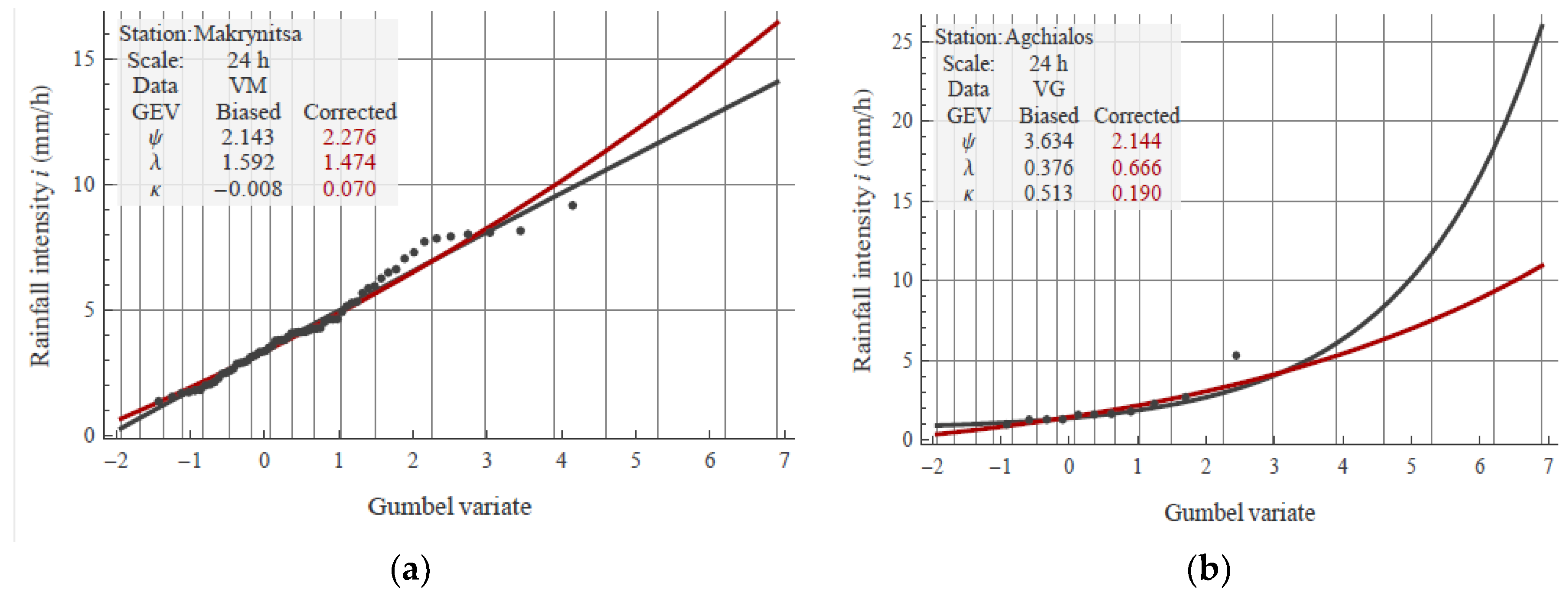
At each station, the shape parameter κ is initially obtained by fitting the GEV model to the maximum 24 h data and estimating its parameters by the L-moments method [40,41]. Next, we employ the correction technique developed by [42], in order to adjust the biased estimations of κ, thus prohibiting both the use of too high values and the generation of negative values, which are unfeasible, since the maximum rainfall cannot be bounded. We remark that such inconsistencies are mainly due to sample uncertainties, which are induced due to the small size of the observed rainfall maxima, the existence of outliers as well as measurement errors.
Step 3:
Based on their point values of parameter κ, we employed a geographical classification of the stations to obtain regional values that are associated with climatic and topographic characteristics.
Step 4:
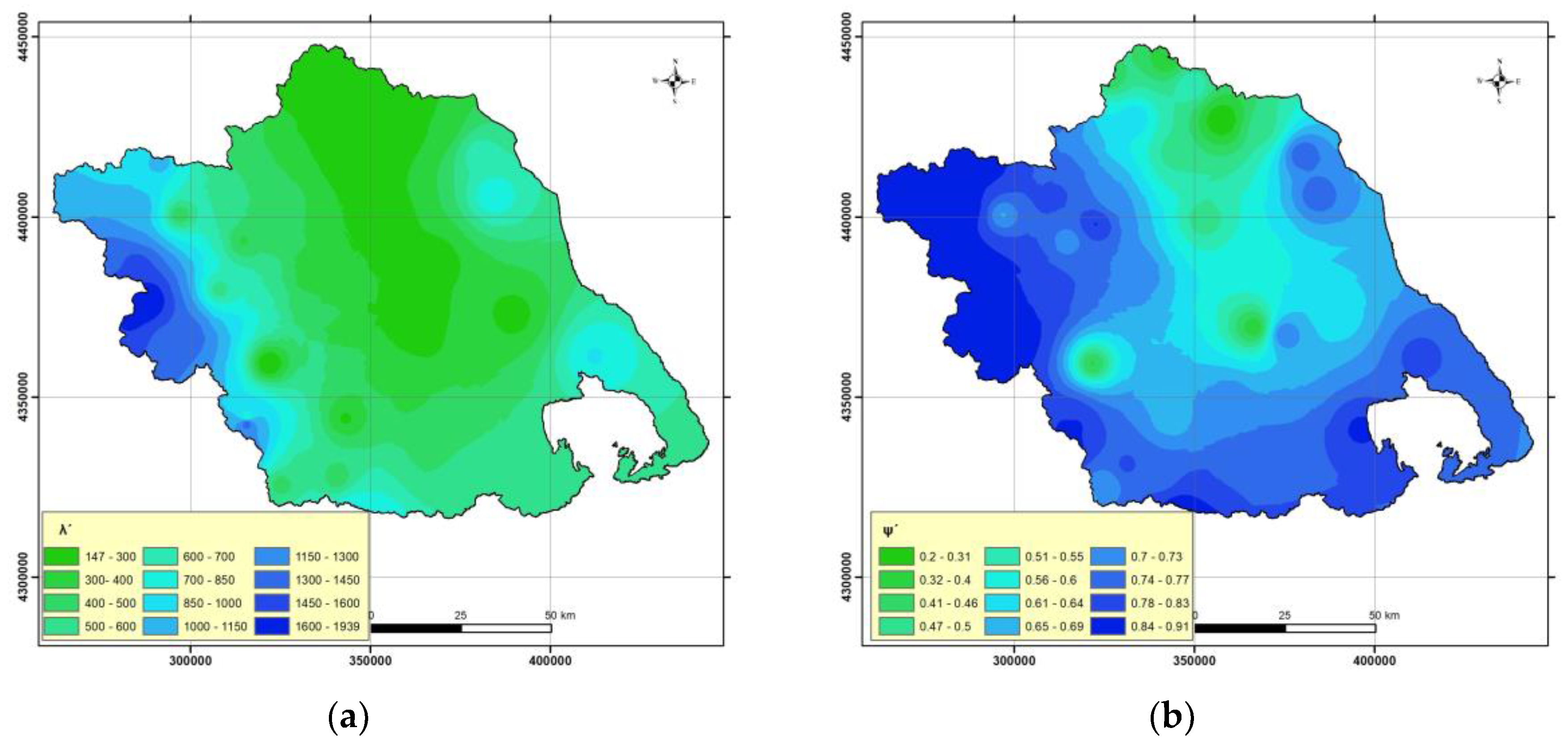
For given parameters κ, η and θ, we employed the L-moments method to estimate the scale and location parameters, λ′ and ψ′, at each station.
In order to extract the confidence intervals of rainfall estimations, we employed a generalized Monte Carlo framework, since for the GEV distribution (as made for most of distributions) there are no analytical formulas [43]. Let Χ be a random variable following a distribution function F X , θ the parameters of this distribution that have been estimated by a sample of n values of X, and u and γ are the desirable exceedance probability and confidence level, respectively. The computational procedure is the following:
Step 1:
Using an appropriate generator of random numbers following the desirable distribution F X , we produce m synthetic samples x i = { x i 1 , x i 2 , …, x i n }, where n is the length of the historical data.
Step 2:
From each synthetic sample xi we estimate its statistical characteristics and the corresponding sample parameters θ i of F X , by applying the same procedure with the historical data (e.g., method of moments, L-moments, maximum likelihood, etc.).
Step 3:
For the desirable probability u, we generate m synthetic values using the inverse cumulative distribution function, i.e.:
x i ( u )   =   F X 1 ( θ i ,   u )
Step 4:
We estimate the confidence limits x U (u) and x L (u), by computing the larger m (1 − γ)/2 and smaller m (1 + γ)/2 values of the sorted sample of x i (u).
In the context of our analyses, at each station we initially extracted the compound sample of rainfall maxima, derived by multiplying each individual set of duration d by the duration function b(d) = ( 1 + d / θ ) η . According to Equation (1), the derived data follows a Pareto distribution function, with parameters λ′, ψ′, κ, given by:
F X   =   1     ( x / λ   +   ψ ) 1 / κ
In the context of Monte Carlo simulations, for each station we employed the inverse function of Equation (3) to generate 20,000 sets of synthetic rainfall data from the Pareto distribution, with length equal to the historical one. This function is given by:
x ( u )   =   F X 1 ( u )   =   λ   [ 1 ( 1 u ) κ     ψ ]
Next, from each set we estimated the parameter values λ′, ψ′, κ, and associated confidence limits x U (u) and x L (u) for T = 50, 100 and 1000 years (or u = 0.980, 0.990 and 0.999, equivalently). By setting γ = 80%, we obtained the 2000th smallest and largest value, respectively. Given that the confidence values refer to the compound sample, they are standardized against the duration. In order to obtain the desirable rainfall value for a specific duration, the derived values of x U (u) and x L (u) are multiplied by:
ξ ( d )   =   d ( 1 + d / θ ) η
Using averaged IDF parameters and associated confidence limits per sub-basin we formulated the design storm hyetographs of 24 h duration, by employing two typical time profiles, i.e., the alternating block method, for T = 50 and 100 years, and the worst profile method, for T = 1000 years [44,45,46]. Both approaches require the estimation of partial rainfall depths for durations Δt, 2Δt, …, N Δt = D, which are appropriately allocated to formulate a hypothetical hyetograph that preserves the desirable return period at all temporal scales.

3.3. Hydrological Model Assumptions and Representation of Uncertainties

For each return period of interest (T = 50, 100, 1000 years) we have formulated three scenarios (herein referred to as low, average and high), in order to account for joint rainfall and hydrological uncertainties. In particular, we assumed that the design rainfall estimations provided by the IDF relationship correspond to the average scenario, while its 80% confidence limits, which are measure of rainfall uncertainty (more precisely, parameter uncertainty of the IDF expression), correspond to the two extreme scenarios. On the other hand, the hydrological uncertainty has been expressed in terms of three typical antecedent soil moisture conditions (dry, moderate, wet) that are employed within the rainfall-runoff modelling approach, as explained next. In this respect, we have formulated 3 × 3 = 9 scenarios, in total.
The transformation of the hyetograph to flood runoff was made by subtracting the hydrological deficits (i.e., the part of rainfall that is initially intercepted in the ground and by the canopy, and is then either infiltrated or evaporated), thus obtaining the so-called effective rainfall or rainfall excess. In this respect we employed the well-known SCS-CN approach, developed by the Soil Conservation Service [12]. This method uses two parameters, i.e., the maximum potential retention, S, and the initial abstraction, h a 0 , to estimate the evolution of effective rainfall through the empirical formula:
h e   =   ( h   h a 0 ) 2 h     h a 0 + S
According to the standard SCS approach, we set h a 0 = 0.20 S, which is the threshold for surface runoff generation. Under this premise, the sole parameter of the method is the maximum potential retention of each sub-basin, estimated by the well-known formula:
S = 254   ( 100 C N 1 )
where CN is the spatially-averaged curve number value of each specific sub-basin. The latter has been extracted on the basis of distributed soil and land cover information, following the typical classification by NRCS [47], by means of detailed lookup tables. In order to account for the soil moisture present in the soil profile before the start of an event, the SCS-CN method considers three antecedent soil moisture conditions types (AMC I, AMC II, and AMC III), referring to dry, average or wet conditions, respectively, which depend on the total 5-day antecedent rainfall and the season category (dormant or growing). The CN values given in lookup tables (hereafter symbolized CN II) refer to average conditions, while for the other two AMC types, SCS provides empirical conversion formulas to estimate the parameter value for dry (CN I) and wet conditions (CN III) In the proposed framework, the CN values for dry and wet conditions, combined with the low and upper confidence limits of rainfall, were used to generate design hyetographs that have been used to quantify the uncertainty around the “standard” (i.e., average) hydrological scenario.
For the transformation of the excess rainfall over the sub-basin to flood hydrograph at the outlet junction, we applied the unit hydrograph (UH) approach, using the dimensionless curvilinear unit hydrograph by NRCS (also referred to as Standard PRF 484), in which the time and discharge are expressed as ratios of time to peak and peak discharge, respectively. Key assumptions are that 37.5% of the total flood volume is produced within the rising limb, while the base time, t b , is considered five times the time to peak, t p . The UH is fully determined in terms of lag time, t L , defined as the time distance from the centroid of the unit hydrograph of duration d, from the centroid of unit rainfall, which is by definition equal to d/2. Assuming also that t L = 0.6 t c , where t c is the time of concentration, and under the assumption that the centroid of the unit hydrograph is approximately located in the peak, we approximate the time of peak by:
t p   =   d / 2   +   0.6 t c
Moreover, given that t b = 5 t p , and by employing the mass balance equation for total volume equal to the effective rainfall volume, we can also estimate the peak discharge by:
q p   =   2.08   A / t c
where A is the basin area (in km2).
According to widespread flood modelling practices for ungauged basins, t c is characteristic time quantity of a river basin, typically defined as the longest travel time of the surface runoff from the hydraulically most remote point of a basin to its outlet, and computed by empirical formulas that estimate the basin response time as function of its geomorphological characteristics. A widely used empirical approach is the Giandotti formula, given by:
t c = 4 A + 1.5 L 0.8 Δ z
where tc is the time of concentration (h), Α is the basin area (km2), L is the length of the longest runoff distance across the basin (km), and Δz is the difference between the mean elevation of the basin and the outlet elevation (m). This formula has been proved quite suitable for reproducing observed peak flood flows in a number of small river basins in Cyprus; in particular, its predictive capacity was by far superior with respect to other widely-used empirical formulas of the literature [13]. In the study, we used the time of concentration, estimated by the Giandotti formula, as the reference response time of each area of interest, i.e., the entire catchment and its sub-basins. The computation of the associated geometric quantities A, L and Δz was estimated via typical processing tools in GIS environment. In the case of complex river networks, i.e., with confluences, we considered the longest flow path across each corresponding area.
Theoretical proof and empirical evidence imply that tc is definitely not a constant property of the basin, but it varies significantly with the flow [13,48]. In fact, the variability of tc is explained by the dependence of the kinematic wave celerity on the flow rate. Apparently, as surface runoff increases, the flow velocity across the river network and its tributaries also increases, which results in a faster response of the basin. For instance, [49] analyzed a large number of flood hydrographs and found that tc varied by even one order of magnitude across flood events of different intensities. To account for the dependence of the response time of the basin against runoff, we employed the following semi-empirical formula, which arises from the kinematic wave theory, considering that tc is inversely proportional to the design rainfall, i.e.,
t c ( T )   =   t c i ( 5 ) i ( T )
where i(5) is the design rainfall intensity for return period Τ = 5 years, for which the time of concentration is estimated by the Giandotti formula, and i(Τ) is the intensity of any higher return period, T. In this respect, the “reference” time of concentration by the Giandotti formula is assumed valid for high and medium frequency flood events, yet for low-frequency events, which interest hydrological design, this time has to be reduced. Evidently, as the time of concentration reduces, all associated time quantities are similarly reduced, namely, the lag time, the time to peak and the base time of the unit hydrograph. In fact, smaller lag times result in much narrower unit hydrographs, which in turn results in increased peak discharge, in order to preserve the unit flood volume. An example involving a hypothetical river basin is provided in Figure 3. This approach is definitely more consistent with reality, since it accounts for nonlinearities in runoff routing, which are ignored by the unit hydrograph theory.

3.4. Hydraulic-Hydrodynamic Modelling

The two dimensional (2D) HEC-RAS model was developed by the Hydrologic Engineering Center (HEC) of United States Army Corps of Engineers [50] and has been applied in many studies for flood inundation modelling (e.g., [9,10,25,26,27,51,52,53,54]). Moreover, a benchmark analysis based on the two dimensional modelling capabilities, conducted by the U.S. Army Corps of Engineers, proved that HEC-RAS performed extremely well compared to the leading 2D models [55]. Therefore, the 2D HEC-RAS hydraulic-hydrodynamic model has been selected for flood inundation and mapping.
The HEC-RAS 5.0.3 computational engine is based on the full 2D Saint-Venant equations or the 2D diffusive wave equations [50]. Shallow water equations are simplifications of the Navier-Stokes equations. The basic assumptions that are followed in order to approximate the turbulent motion using eddy’s viscosity are: (a) Reynolds averaged equation is used, (b) the flow is incompressible, (c) the density and the hydrostatic pressure are uniform and d) the horizontal length scale is bigger than the vertical length scale. Therefore, the application of these assumptions to the Navier-Stokes equations results to the differential form of Shallow Water equations [50]. The advection, viscous, and unsteady terms can be neglected in cases where the main terms of momentum equations are the bottom friction terms and the barotropic pressure gradient (gravity) term, resulting in the transformation of the momentum equation to a two-dimensional form of the Diffusion Wave Approximation. Thus, the Diffusive Wave Approximation of the Shallow Water (DSW) equations can be derived through the combination of mass conservation and the two-dimensional form of the Diffusion Wave Approximation. Finally, HEC-RAS 2D solver is using the sub-grid bathymetry approach [50].
The combination of the above assumptions results in an almost hydrostatic pressure and minor vertical velocity. In cases where strong wind forcing exists, the pressure is non-hydrostatic, and the baroclinic pressure gradients (variable density) are absent, a vertically-averaged version of the momentum equation is suitable. Given these conditions, the shallow water equations can be obtained by excluding the terms of vertical derivative and the vertical velocity. Accordingly, the momentum equations are expressed as follows [50]:
u t + u u x + v u y = g H x + v t ( 2 u x 2 + 2 u y 2 ) c f u + f v
v t + u v x + v v y = g H x + v t ( 2 v x 2 + 2 v y 2 ) c f v + f u
where u and v are the velocities in the Cartesian directions; g is the gravitational acceleration; vt is the horizontal eddy viscosity coefficient; cf is the bottom friction coefficient; and f is the Coriolis parameter.
One of the basic factors of input data uncertainty in flood inundation modeling and mapping, especially when 2D hydraulic hydrodynamic models are used, is the Digital Elevation Model (DEM) accuracy. The DEM estimation process involves several errors, especially in complex river and riverine areas, due to the topographical technique used [10,25,26,56]. The most common approaches followed for the river and riverine areas topography estimation and the DEM generation are ground surveying topographic approaches and photogrammetric techniques. However, the use of such techniques in flood inundation modelling, especially in complex river topographies involve some limitations such as the small spatial extent and the possibility to produce several errors and affect the accuracy of the produced DEM [57,58]. These limiting factors can be minimized with the use of high accuracy aerial photographs or orthophotos. The high accuracy aerial photographs or orthophotos can produce acceptable DEM resolutions for large scale flood inundation modelling and mapping at ungauged urban areas [59]. In this study, the DEM resolution used is 5 m and has been provided by National Cadastre and Mapping Agency S.A. (NCMA). The geometric resolution of the DEM is RMSEz ≤ 2.00 m with absolute accuracy ≤ 3.92 m for 95% confidence level. The raw data consist of the Digital Surface Model that includes canopy, manmade structures and other surface obstacles. First, the different DSMs derived from the 1:5000 aerial photos have been merged to a continue DSM. Then, the entire DSM has been processed to fill/sink the erroneous areas. Finally, the DSM has been re-corrected using typical elevation downgrading methods in order to create the DEM.
An important input data uncertainty factor in flood inundation modelling is the roughness coefficient and the parameterization process that follows. A typical approach for large scale applications that uses two-dimensional hydraulic models is the estimation of the roughness coefficient using CORINE land cover data and standard roughness coefficient tables (e.g., [30]). Therefore, in this study the average values of Manning’s roughness coefficient (Table 1) have been estimated using CORINE land cover classification in combination with typical Manning’s roughness coefficient tables [60]. Moreover, based on the EU Flood Directive guides the “upper” and “lower” boundaries of Manning’s roughness coefficient were estimated. The “upper” and “lower” boundaries are estimated as −50% and +50% of the average Manning’s roughness coefficient values (Table 1), respectively. Furthermore, a significant factor in hydraulic-hydrodynamic modelling applications for engineering purposes is the accurate representation of the river and riverine area hydraulic structures (bridges, culverts, weirs, flood protection works, etc.). Thus, all hydraulic structures of the study area were detected using aerial photographs, a GIS database of the technical works, field observations and information collected by several authorities. Then, the important hydraulic structures have been selected for accurate topographical survey based on the following guides:
  • Hydraulic structures close to erroneous DEM area.
  • Hydraulic structures close to historical flood points.
  • Hydraulic structures inside the Potential High Flood Risk Areas [34].
  • Hydraulic structures close to recently recorded flood episodes.
  • Hydraulic structures that accurate topographical data are absent.
  • Hydraulic structures within main water bodies.
Then, based on hydraulic structures geometry data, the entire DEM has been modified in order to include the flood protection works and the geometry of all hydraulic structures. Moreover, the two-dimensional HEC-RAS hydraulic-hydrodynamic model is capable of the representation of the bridges as a combination of culverts and weirs and to calculate water surface profiles for several system formulations [50].
Finally, flood inundation modelling and mapping at urban and suburban areas remains a big challenge due to the complexity of the entire system. Also, the hazardous effect of floods in urban and suburban areas has a significant social impact, big economic losses, and in some cases fatalities [1]. One of the most important factors in flood inundation modelling in built up areas is the building representation within the 2D hydraulic-hydrodynamic model. The most common building representation methods assume that each cell of the mesh/grid that is located inside a building block area is represented as [61,62,63,64]: (1) Solid object; (2) with local increase of the elevation; (3) with higher roughness coefficient values. In the solid representation method of the building blocks, the flow eliminates within the solid block. This can be achieved with several methods that depends on the numerical scheme used. In the local increase of building block representation method, each building block is modified in the DEM in order to have bigger elevation than the bare earth altitude. The third approach of building representation involves either the local rise of roughness coefficient (i.e., Manning, Chézy, Darcy-Weisbach) for the building blocks areas or by adding supplementary parameters of porosity and building drag coefficient to the numerical scheme of the model [63]. Recent studies concerning the building block methodologies [64] showed that all methods have advantages and disadvantages and none of them prevail among the others. Therefore, in this study that deals with large-scale applications, the second (local increase of the elevation) building block representation method has been selected.

3.5. Hydraulic Simulation of Lower Course of Volos City Streams and Evaluation Procedure

The methodology developed for large-scale fluvial flood inundation modelling applications for ungauged urban areas is applied in three streams (Xerias, Krafsidonas, Anavros) that cross Volos city, Greece (Figure 1). Typical techniques and methods for ungauged streams were used for the hydraulic-hydrodynamic modelling configuration. Because of severe lack of flood data, the proposed methodology is validated using a simulated historical flood event only for Xerias stream reaches. The application of the hydraulic simulation of the lower course of Volos city streams is described in the next paragraphs.
Xerias model domain (Figure 2) extends downstream of junction J4, and involves three reaches (J4-J2, J3-J2, J2-J1), while Krafsidonas and Anavros hydraulic model simulations extend downstream of their respective junction J2, and involve one reach per stream (J2-J1). The total length of the simulated stream reaches is approximately 8.5 km, 3.7 km, and 2.2 km for Xerias, Krafsidonas and Anavros, respectively. All examined reaches are crossing urban areas of Volos city. The HEC-RAS 2D model was used for flood inundation modelling and mapping with: (a) flexible mesh computation point spacing (Xerias = 14 m/Krafsidonas = 5 m/Anavros = 5 m), (b) 2D diffusion wave solution, and (c) computation interval 2 s. The input DEM spatial resolution used in this study is 5 m and in some cases where extensive flood mitigation works exist has been downgraded to 1 m. All building blocks of Volos city were represented with a 30 m local increase of the elevation (elevation rise method).
A significant problem of flood mitigation works and hydraulic structures (bridges, culverts, weir, etc.) representation in 2D flood inundation modelling is the pixel size and their false description within the DEM. A non-detailed DEM spatial resolution (big pixel size) in combination with the appearance of natural or artificial structures close to the flood mitigation works and hydraulic structures can lead to distortions of the elevation and by extension to their false representation within the DEM. In cases where the actual topography of the flood mitigation works and hydraulic structures exist, the limitation mentioned above can be eliminated with DEM editing. This study uses the XS interpolation surfaces module (HEC-RAS/RAS-Mapper) for DEM editing and by extension, the precise representation of flood mitigation works and hydraulic structures (bridges, culverts, weir, etc.) [65]. For better mesh resolution close to flood mitigation works and hydraulic structures, several Breaklines elements have been added. During the mesh generation process, the Breaklines elements force the orientation and the construction of cell faces along with them. Therefore, with the use of Breaklines elements the mesh is enforced near to flood mitigation works, hydraulic structures, and the building block areas [65].
Concerning the important hydraulic structures of the study areas, 10, 20 and 4 bridges have been taken into account in flood inundation modelling for Xerias, Krafsidonas, and Anavros streams, respectively. Inputs of hydraulic modeling were hydrographs provided by average hydrological simulation scenarios, using “average” roughness coefficients that were estimated according to CORINE 2000 land use classes. For all return periods, apart from the hydrographs provided by the lower and upper scenarios, we also perturbed the roughness values by −50% and +50%, respectively, to obtain overall uncertainty bounds of inundated areas and associated hydraulic quantities, i.e., water depths and velocities.
A typical process followed in cases where severe lack of flood data exist is the use of qualitative criteria that are based on matching agreement of the 2 × 2 contingency table (Simulated vs. Observed) [7,10,17,25,26,66,67]. In this study the qualitative criterion Threat Score (TS) or Critical Success Index (CSI) [68] has been selected for the validation of the flood inundation modelling results. CSI is estimated by the 2 × 2 contingency table for all grids as following:
C S I =   A ( A + B + C )
where A = Hit—event simulated to occur, and did occur, B = False alarm—event simulated to occur, but did not occur and C = Miss—event simulated not to occur, but did occur. Recent studies identified CSI as an efficient validation measure in flood inundation modelling and mapping when the focus is on the flood extent spatial distribution [7,10,25,26,66,67]. In this study, simulated flood inundation data that were derived from a historical flash flood event were used for validation and evaluation of the proposed methodology [10,25,26,35]. The CSI is used for the comparison of the inundated area between the constructed T = 100 year flood and the simulated historical flood event of approximately T = 100 year.

4. Volos City: Application and Results of the Modelling Framework

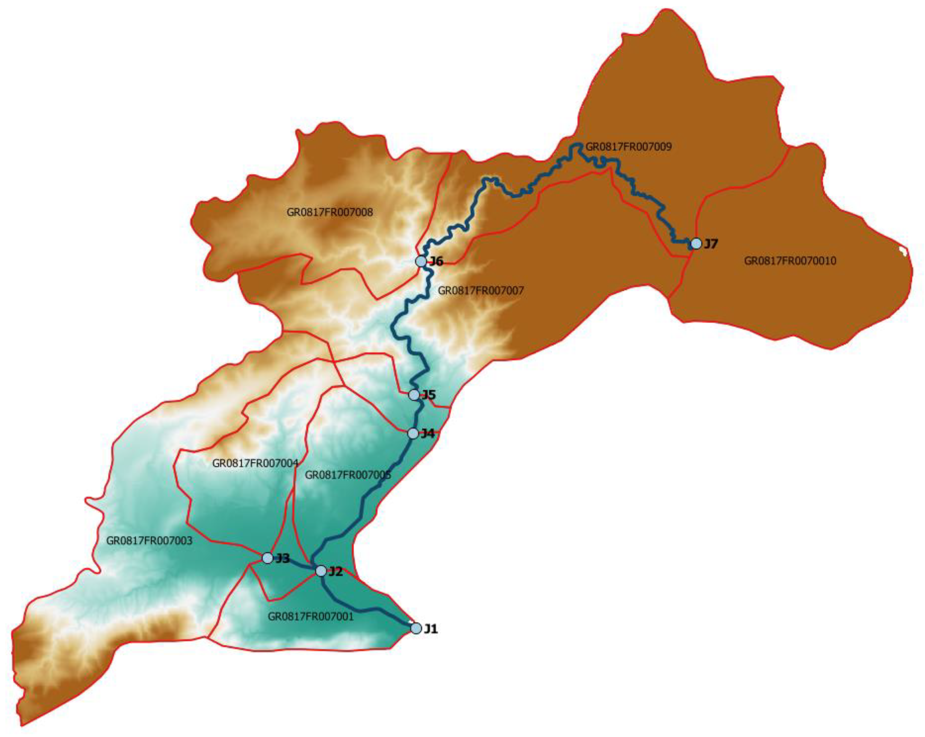
4.1. Semi-Distributed Hydrological Modelling of Volos City Watersheds

The parameters of the ombrian curves (Equation 1) for the design rainfall were estimated on the basis of extreme rainfall data at 57 meteorological stations across the River Basin District of Thessaly, comprising 224 samples of annual maxima at several time scales. Initially, we estimated the two parameters of the duration function, using finely-resolved rainfall maxima from the 15 recording stations. The optimal values of the two parameters were θ = 0.042 και η = 0.639, which have been considered constant over the broader Thessaly. On the other hand, the estimation of the three parameters of the return period expression was based on 24-h data at 56 stations. In Figure 4, we contrast the initial and adjusted fitting of the GEV distribution to the daily rainfall maxima at the closest stations of the study area, i.e., Makrynitsa and Agchialos. In the first station, the initial estimation of parameter κ was −0.008, which has been corrected to 0.007, while in the second station the initial estimation was 0.513 (which is attributed to the very high value of the largest observed rainfall), which has been reduced to 0.190. The rainfall stations were next grouped into three climatic zones and assigned a representative value of κ. In particular, the three study basins are located at the median zone, with κ = 0.09. Accounting for the given values of parameters θ, η and κ, we finally provided point estimations of scale and location parameters λ′ and ψ′, respectively, and we also generated empirical 80% confidence intervals of point rainfall estimations for T = 50, 100 and 1000 years, by employing Monte Carlo simulations against the scale and location parameters λ′ and ψ′.
In Table 2 we show the point estimations at Makrynitsa and Agchialos, and the 80% confidence limits for the 24 h rainfall, for the three return periods of interest. We assigned the same values for parameters κ, θ and η, i.e., 0.092, 0.042 and 0.639, respectively, while for the rest two parameters of the IDF relationship we used λ′= 881.0 and ψ′= 0.788 for Makrynitsa, and λ′= 565.2 and ψ′= 0.840 for Agchialos.
Using the point estimations of λ′ and ψ′, and the associated confidence limits of rainfall, we provided maps of distributed parameters over Thessaly (Figure 5), which allowed extracting spatially-distributed design rainfalls across the study catchments. In particular, we averaged the associated IDF parameters and standardized confidence limits over each sub-basin area, and next employed either the alternating block method (for T = 50 and 100 years) or the worst profile method (for T = 1000 years) in order to formulate the corresponding hyetographs.
Since the parameters of IDF curves, which are inputs for the estimation of design storms, have been estimated on the basis of the point data, they are valid at the point scale. However, it is well-known that for any given return period and duration, the spatially averaged rainfall over a given area is less than the maximum point rainfall depth. For this reason, we have reduced the point rainfall estimations, to provide areal estimations over the corresponding sub-basins, by applying a commonly used adjustment approach, based on the so-called areal reduction factor, φ. The latter is a dimensionless parameter, defined as the ratio of areal to point rainfall, which is decreasing function of the area and increasing function of duration. To facilitate calculations, we used the analytical formula by Koutsoyiannis and Xanthopoulos [69]:
φ = m a x ( 1     0.048 A ( 0.36     0.01   ln A ) d 0.35 ,   0.25 )
where Α is the area in km2 and d is the rainfall duration in h. The above empirical relationship has been formulated on the basis of tabular data by UK-NERC [70], which captures a wide range of durations (in particular, from 1 min to 25 days) and catchment sizes (from 1 to 30,000 km2). For instance, in the study basin of Xerias, with A = 116.8 km2, we employed φ = 0.788 and 0.930, in order to reduce the design rainfall estimations for durations 1 and 24 h, respectively.
In Table 3 we present the CN values that have been applied across the ten sub-basins of Xerias for the three AMC types, corresponding to the three hydrological scenarios of this study. It is interesting to highlight that the basin exhibits significant heterogeneity, since their CN II values range from 50 to 82, while the uncertainty induced to AMC is amplified in the areas with low CNs.
The application of the semi-distributed hydrological modelling procedure in the three watersheds led in the estimation of design hydrographs at the junctions used for the hydraulic simulation for all examined hydrologic conditions and return periods. For example, Figure 6 shows the design hydrographs at the outlet of Xerias watershed (Junction J1) for average soil moisture conditions (CN II) for the three study return periods. Similar design hydrographs were estimated for all examined junctions at the study area with similar shapes, but with different peak magnitudes.

4.2. Hydraulic Modelling of Lower Course of Volos City Streams

An operational method for Floods Directive implementation in ungauged urban areas is applied for different return periods (T = 50, 100, and 1000 years), three hydrologic conditions (AMCI, AMCII, AMCIII) that correspond to lower, average and upper estimations of the design rainfall, respectively, and three roughness values (−50%, average, +50%). The examined scenarios aim to quantify the uncertainty induced to extreme rainfall analysis, antecedent soil moisture conditions and estimations of the roughness coefficient. Thus, this study investigates nine (9) different operational scenarios that incorporate important (yet not all) aspects of the total model uncertainty.
Due to lack of data, the methodology has been evaluated only for Xerias stream, based on the historical flood event that occurred October 9th, 2006. The observed hydrograph was estimated in previous works [10,25,26,35] and considered to correspond to an approximately 100 years flood event. The comparison of the simulated historical flood event and the simulated average design flood scenario (AMCII, T = 100, average roughness value) is examined in the validation procedure with the skill score Critical Success Index. Table 4 presents the flooded areas (km2) per river reach and the total flooded extent of Volos city for all examined hydrologic and hydraulic scenarios at the selected return periods. Flood extent variations that are presented in Table 4, and depicted in Figure 7 and Figure 8, show that the hydrologic conditions scenarios, accounting for both rainfall and initial soil moisture uncertainty, have much stronger impact on the flood extent than the return period itself, which is only an indicator of the rainfall risk. Specifically, the flood extent ranges between 0.068 km2 and 2.76 km2 for dry (AMCI) conditions, from 0.21 km2 to 6.01 km2 for average (AMCII) conditions, and from 0.77 km2 to 9.7 km2 for wet (AMCIII) conditions (Table 4, Figure 7). This outcome is not surprising and confirms that the generation of a flood is strongly influenced by the soil moisture that is already stored at the beginning of rainfall.
Furthermore, based on the return period discretization it is observed that flood extent results of 50 and 100 years are very close to each other and the highest flood extent values with significant difference from the other return periods presented in 1000-year return period (Table 4, Figure 7). Specifically, the flood extent of all examined scenarios ranges between 0.068 km2 and 5.3 km2 for T = 50 years, from 0.081 km2 to 6.34 km2 for T = 100 years, and from 0.21 km2 to 9.7 km2 for T = 1000 years (Table 4, Figure 7 and Figure 8). Figure 9 presents the simulated velocities only for average configurations of input rainfall, soil moisture conditions and roughness coefficients of return period: (a) T = 50 years, (b) T = 100 years, (c) T = 1000 years. Finally, the validation procedure that is based on the comparison between Xerias stream flood extent of the designed flood of T = 100 by employing the average input rainfall, soil moisture conditions and roughness coefficients and simulated flood extent of the 2006 historical flash flood event achieved a score in Critical Success Index of 0.77 and shown on Figure 10. This high score of CSI justifies the accuracy of the proposed operational methodology for flood directive implementation in urban and ungauged areas.
Overall, in the context of flood inundation and mapping, this study tried to quantify the following major sources of uncertainty: (1) statistical uncertainty associated with the parameters of IDF relationships (i.e., scale and location parameters), originating from limited samples of observed extreme rainfall data; (2) hydrologic uncertainty associated with the initial soil moisture conditions of the hydrological model, resulting to a wide range of the key input parameter of the SCS-CN method, i.e., the potential maximum retention; and (3) parametric uncertainty associated with Manning’s roughness coefficient, which is a typical input in all hydraulic simulation models. Results are quite diverse, since the uncertainty bounds of all key flood quantities (peak flows, flood volumes, inundated areas, etc.) strongly overlap the risk expressed in terms of return period of rainfall, while for large return periods, the lower and upper estimations may differ by one order of magnitude. Special attention should be given to the developed methodology and its application only for specific return periods and hydrologic-hydraulic conditions due to the great variability in the peak discharge estimation. A comparison of several methods and conditions prior to the decision-making phase could be proven useful flow flood management purposes. Hence, an ensemble of methods and scenarios should always be applied for engineering purposes, in order to choose the most appropriate technique in relation to the flood prone areas and proposed flood protection measures.

5. Concluding Remarks

In order to reduce the risk and adverse consequences of floods, the EU issued the so-called Flood Directive 2007/60/EC. Its implementation requires a proper estimation of flood hazards and representation of potential risks, which in turn makes essential the use of reliable hydrological methodologies for the estimation of associated flood quantities, as well as suitable and efficient hydraulic simulation tools for flood inundation modelling and mapping. In ungauged basins of relatively small extent that mainly affected by fluvial flash floods, which are the case in Greece, data-driven approaches in flood risk assessment, based on statistical analysis of observed floods, are not feasible. For this reason, flood estimations are exclusively estimated through classical engineering approaches, following the event-based deterministic paradigm.
In this study, a methodological approach for implementing the EU Floods Directive in Greece is developed, emphasized for flood risk management in urban areas, which is demonstrated for the Volos city case, where frequent flood episodes are observed. The methodology is based on typical hydrological and flood inundation modelling and mapping techniques for ungauged catchments. Spatially-distributed design hyetographs are applied for hydrologic and hydraulic 2D modelling of floods taking into account parametric and structural uncertainty. The average scenario against a simulated historical flood extent data was validated through the objective qualitative criterion of CSI that is counting the spatial distribution of the flooded area.
According to the flood extent values, it seems that the uncertainty induced in hydrological modeling, with respect to extreme rainfall estimations and antecedent soil moisture conditions, dominates against the return period. We remark that these two components are not the sole sources of uncertainty within rainfall-runoff transformations. This makes it essential to move to more rigorous methodological approaches (e.g., stochastic), instead of quantifying the flood risk on the basis of the return period of rainfall.
The overall results also proved that sensitivity analysis should be a mandatory process in flood modelling and mapping for urban areas due to the variation of the results because of the hydrologic conditions or the selected return period that is used. Finally, the results indicate the uncertainty introduced in flood risk management in urban areas using typical engineering practices.

Acknowledgments

This paper is part of the project “Management Plans of Flood Risks for River Basins in Thessaly, Western Sterea Hellas and Epirus Regions, Greece” co-funded by E.U. and the Greek Ministry of Energy and the Environment. This project constitutes the implementation of the EU Directive on floods (E.C. 2007/60) in the above regions of Greece. The research presented in the paper is partially supported by this project. The authors would like to thank the guest editors for their kind invitation and the three anonymous reviewers for their constructive and useful comments, which contributed to an improved presentation of the paper.

Author Contributions

G.P., A.E., L.V., and A.L. designed the study, developed the methodology, and wrote the manuscript. S.M.P., A.K., I.T. and P.K. performed the IDF analysis and contributed to the hydrologic analysis part. Furthermore, G.P. performed the hydraulic simulation and validation of the study area.

Conflicts of Interest

The authors declare no conflict of interest.

References

  1. Tsakiris, G. Flood risk assessment: Concepts, modelling, applications. Nat. Hazards Earth Syst. Sci. 2014, 14, 1361–1369. [Google Scholar] [CrossRef]
  2. Hall, J.; Arheimer, B.; Borga, M.; Brázdil, R.; Claps, P.; Kiss, A.; Kjeldsen, T.R.; Kriauĉuniene, J.; Kundzewicz, Z.W.; Lang, M.; et al. Understanding flood regime changes in Europe: A state-of-the-art assessment. Hydrol. Earth Syst. Sci. 2014, 18, 2735–2772. [Google Scholar] [CrossRef] [Green Version]
  3. Kreibich, H.; Di Baldassarre, G.; Vorogushyn, S.; Aerts, J.C.J.H.; Apel, H.; Aronica, G.T.; Arnbjerg-nielsen, K.; Bouwer, L.M.; Bubeck, P.; Caloiero, T.; et al. Earth’s Future Special Section : Adaptation to flood risk : Results of international paired flood event studies. Earth’s Future 2017, 5, 953–965. [Google Scholar] [CrossRef]
  4. Diakakis, M.; Mavroulis, S.; Deligiannakis, G. Floods in Greece, a statistical and spatial approach. Nat. Hazards 2012, 62, 485–500. [Google Scholar] [CrossRef]
  5. Centre for Research on the Epidemiology of Disasters (CRED). Summarized Table of Natural Disasters in Greece from 1900 to 2017, EM-DAT: The CRED/OFDA International Disaster Database–www.emdat.be–Université Catholique de Louvain–Brussels–Belgium. Available online: http://www.emdat.be (accessed on 12 January 2018).
  6. Apel, H.; Thieken, A.H.; Merz, B.; Blöschl, G. Flood risk assessment and associated uncertainty. Nat. Hazards Earth Syst. Sci. 2004, 4, 295–308. [Google Scholar] [CrossRef]
  7. Aronica, G.; Bates, P.D.; Horritt, M.S. Assessing the uncertainty in distributed model predictions using observed binary pattern information within GLUE. Hydrol. Process. 2002, 16, 2001–2016. [Google Scholar] [CrossRef]
  8. Aronica, G.T.; Franza, F.; Bates, P.D.; Neal, J.C. Probabilistic evaluation of flood hazard in urban areas using Monte Carlo simulation. Hydrol. Process. 2012, 26, 3962–3972. [Google Scholar] [CrossRef]
  9. Dottori, F.; Di Baldassarre, G.; Todini, E. Detailed data is welcome, but with a pinch of salt: Accuracy, precision, and uncertainty in flood inundation modeling. Water Resour. Res. 2013, 49, 6079–6085. [Google Scholar] [CrossRef]
  10. Papaioannou, G.; Loukas, A.; Vasiliades, L.; Aronica, G.T. Flood inundation mapping sensitivity to riverine spatial resolution and modelling approach. Nat. Hazards 2016, 83, 117–132. [Google Scholar] [CrossRef]
  11. Teng, J.; Jakeman, A.J.; Vaze, J.; Croke, B.F.W.; Dutta, D.; Kim, S. Flood inundation modelling: A review of methods, recent advances and uncertainty analysis. Environ. Model. Softw. 2017, 90, 201–216. [Google Scholar] [CrossRef]
  12. Soil Conservation Service (SCS). National Engineering Handbook; Section 4, Hydrology (NEH-4); U.S. Department of Agriculture: Washington, DC, USA, 1972.
  13. Efstratiadis, A.; Koussis, A.D.; Koutsoyiannis, D.; Mamassis, N. Flood design recipes vs. reality: Can predictions for ungauged basins be trusted? Nat. Hazards Earth Syst. Sci. 2014, 14, 1417–1428. [Google Scholar] [CrossRef]
  14. Gr̈aler, B.; Van Den Berg, M.J.; Vandenberghe, S.; Petroselli, A.; Grimaldi, S.; De Baets, B.; Verhoest, N.E.C. Multivariate return periods in hydrology: A critical and practical review focusing on synthetic design hydrograph estimation. Hydrol. Earth Syst. Sci. 2013, 17, 1281–1296. [Google Scholar] [CrossRef] [Green Version]
  15. Horritt, M.S.; Di Baldassarre, G.; Bates, P.D.; Brath, A. Comparing the performance of a 2-D finite element and a 2-D finite volume model of floodplain inundation using airborne SAR imagery. Hydrol. Process. 2007, 21, 2745–2759. [Google Scholar] [CrossRef]
  16. Costabile, P.; Macchione, F. Enhancing river model set-up for 2-D dynamic flood modelling. Environ. Model. Softw. 2015, 67, 89–107. [Google Scholar] [CrossRef]
  17. Horritt, M.S.; Bates, P.D. Evaluation of 1D and 2D numerical models for predicting river flood inundation. J. Hydrol. 2002, 268, 87–99. [Google Scholar] [CrossRef]
  18. Merwade, V.; Cook, A.; Coonrod, J. GIS techniques for creating river terrain models for hydrodynamic modeling and flood inundation mapping. Environ. Model. Softw. 2008, 23, 1300–1311. [Google Scholar] [CrossRef]
  19. Hunter, N.M.; Bates, P.D.; Horritt, M.S.; Wilson, M.D. Simple spatially-distributed models for predicting flood inundation: A review. Geomorphology 2007, 90, 208–225. [Google Scholar] [CrossRef]
  20. Cook, A.; Merwade, V. Effect of topographic data, geometric configuration and modeling approach on flood inundation mapping. J. Hydrol. 2009, 377, 131–142. [Google Scholar] [CrossRef]
  21. Mohammed, J.R.; Qasim, J.M. Comparison of One-Dimensional HEC-RAS with Two-Dimensional ADH for Flow over Trapezoidal Profile Weirs. Casp. J. Appl. Sci. Res. 2012, 1, 1–32. [Google Scholar] [CrossRef]
  22. Néelz, S.; Pender, G.; Britain, G. Desktop Review of 2D Hydraulic Modelling Packages; DEFRA/Environment Agency: Bristol, UK, 2009; ISBN 9781849110792.
  23. Néelz, S.; Pender, G.; Wright, N.G. Benchmarking of 2D Hydraulic Modelling Packages; DEFRA/Environment Agency: Bristol, UK, 2010; ISBN 9781849111904.
  24. Néelz, S.; Pender, G. Benchmarking the Latest Generation of 2D Hydraulic Modelling Packages; DEFRA/Environment Agency: Bristol, UK, 2013; ISBN 9781849113069.
  25. Papaioannou, G.; Vasiliades, L.; Loukas, A.; Aronica, G.T. Probabilistic flood inundation mapping at ungauged streams due to roughness coefficient uncertainty in hydraulic modelling. Adv. Geosci. 2017, 44, 23–34. [Google Scholar] [CrossRef]
  26. Papaioannou, G.; Loukas, A.; Vasiliades, L.; Aronica, G.T. Sensitivity analysis of a probabilistic flood inundation mapping framework for ungauged catchments. Eur. Water 2017, 60, 9–16. [Google Scholar]
  27. Di Baldassarre, G.; Schumann, G.; Bates, P.D.; Freer, J.E.; Beven, K.J. Cartographie de zone inondable: Un examen critique d’approches déterministe et probabiliste. Hydrol. Sci. J. 2010, 55, 364–376. [Google Scholar] [CrossRef]
  28. Sarhadi, A.; Soltani, S.; Modarres, R. Probabilistic flood inundation mapping of ungauged rivers: Linking GIS techniques and frequency analysis. J. Hydrol. 2012, 458, 68–86. [Google Scholar] [CrossRef]
  29. Domeneghetti, A.; Vorogushyn, S.; Castellarin, A.; Merz, B.; Brath, A. Probabilistic flood hazard mapping: Effects of uncertain boundary conditions. Hydrol. Earth Syst. Sci. 2013, 17, 3127–3140. [Google Scholar] [CrossRef]
  30. Dimitriadis, P.; Tegos, A.; Oikonomou, A.; Pagana, V.; Koukouvinos, A.; Mamassis, N.; Koutsoyiannis, D.; Efstratiadis, A. Comparative evaluation of 1D and quasi-2D hydraulic models based on benchmark and real-world applications for uncertainty assessment in flood mapping. J. Hydrol. 2016, 534, 478–492. [Google Scholar] [CrossRef]
  31. Bates, P.D.; Wilson, M.D.; Horritt, M.S.; Mason, D.C.; Holden, N.; Currie, A. Reach scale floodplain inundation dynamics observed using airborne synthetic aperture radar imagery: Data analysis and modelling. J. Hydrol. 2006, 328, 306–318. [Google Scholar] [CrossRef]
  32. Aggett, G.R.; Wilson, J.P. Creating and coupling a high-resolution DTM with a 1-D hydraulic model in a GIS for scenario-based assessment of avulsion hazard in a gravel-bed river. Geomorphology 2009, 113, 21–34. [Google Scholar] [CrossRef]
  33. Bates, P.D.; Horritt, M.S.; Aronica, G.; Beven, K. Bayesian updating of flood inundation likelihoods conditioned on flood extent data. Hydrol. Process. 2004, 18, 3347–3370. [Google Scholar] [CrossRef]
  34. Special Secretariat for Water, Ministry of Environment and Energy (SSW-MEE). Preliminary Assessment of the Flood Directive; Athens: Ministry of Environment and Energy; Available online: http://www.ypeka.gr/LinkClick.aspx?fileticket=T4DDG1hqQMY%3d&tabid=252&language=el-GR (accessed on 12 January 2018).
  35. Papaioannou, G.; Vasiliades, L.; Loukas, A. Multi-Criteria Analysis Framework for Potential Flood Prone Areas Mapping. Water Resour. Manag. 2015, 29, 399–418. [Google Scholar] [CrossRef]
  36. Harats, N.; Ziv, B.; Yair, Y.; Kotroni, V.; Dayan, U. Lightning and rain dynamic indices as predictors for flash floods events in the Mediterranean. Adv. Geosci. 2010, 53, 57–64. [Google Scholar] [CrossRef]
  37. Efstratiadis, A.; Papalexiou, S.M.; Markonis, I.; Mamassis, N. Ombrian curves. In Flood Risk Management Plan of River Basin District of Thessaly (GR08)–Phase A; Special Secretariat for Water, Ministry of Environment and Energy (SSW-MEE): Athens, Greece, 2016. [Google Scholar]
  38. Koutsoyiannis, D.; Kozonis, D.; Manetas, A. A mathematical framework for studying rainfall intensity-duration-frequency relationships. J. Hydrol. 1998, 206, 118–135. [Google Scholar] [CrossRef]
  39. Hirsch, R.M.; Helsel, D.R.; Cohn, T.A.; Gilroy, E.J. Statistical analysis of hydrological data. In Handbook of Hydrology; Maidment, D.R., Ed.; McGraw-Hill: New York, NY, USA, 1993. [Google Scholar]
  40. Hosking, J.R.M. L-Moments: Analysis and Estimation of Distributions Using Linear Combinations of Order Statistics. J. R. Stat. Soc. B 1990, 52, 105–124. [Google Scholar]
  41. Vogel, R.M.; Fennessey, N.M. L moment diagrams should replace product moment diagrams. Water Resour. Res. 1993, 29, 1745–1752. [Google Scholar] [CrossRef]
  42. Papalexiou, S.M.; Koutsoyiannis, D. Battle of extreme value distributions : A global survey on extreme daily rainfall. Water Resour. Res. 2013, 49, 187–201. [Google Scholar] [CrossRef]
  43. Tyralis, H.; Koutsoyiannis, D.; Kozanis, S. An algorithm to construct Monte Carlo confidence intervals for an arbitrary function of probability distribution parameters. Comput. Stat. 2013, 28, 1501–1527. [Google Scholar] [CrossRef]
  44. Sutcliffe, J.V. Methods of Flood Estimation: A Guide to Flood Studies Report; Institute of Hydrology: Wallingford, UK, 1978; Volume 49. [Google Scholar]
  45. Chow, V.T.; Maidment, D.R.; Mays, L.W. Applied Hydrology; McGraw-Hill: Singapore, 1988. [Google Scholar]
  46. Koutsoyiannis, D. A stochastic disaggregation method for design storm and flood synthesis. J. Hydrol. 1994, 156, 193–225. [Google Scholar] [CrossRef]
  47. National Regulator for Compulsory Specifications (NRCS). National Engineering Handbook: Part 630—Hydrology; NRCS: Washington, DC, USA, 2004. [Google Scholar]
  48. Michailidi, E.M.; Antoniadi, S.; Koukouvinos, A.; Bacchi, B.; Efstratiadis, A. Timing the time of concentration: Shedding light on a paradox. Hydrol. Sci. J. 2018, 63. [Google Scholar] [CrossRef]
  49. Grimaldi, S.; Petroselli, A.; Tauro, F.; Porfiri, M. Time of concentration: A paradox in modern hydrology. Hydrol. Sci. J. 2012, 57, 217–228. [Google Scholar] [CrossRef]
  50. Brunner, G. HEC-RAS River Analysis System: Hydraulic Reference Manual, Version 5.0. US Army Corps of Engineers–Hydrologic Engineering Center, 2016a; pp. 1–538. Available online: http://www.hec.usace.army.mil/software/hec-ras/documentation/HEC-RAS%205.0%20Reference%20Manual.pdf (accessed on 12 January 2018).
  51. Alfonso, L.; Mukolwe, M.M.; Di Baldassarre, G. Probabilistic Flood Maps to support decision-making: Mapping the Value of Information. Water Resour. Res. 2016, 52, 1026–1043. [Google Scholar] [CrossRef]
  52. Patel, D.P.; Ramirez, J.A.; Srivastava, P.K.; Bray, M.; Han, D. Assessment of flood inundation mapping of Surat city by coupled 1D/2D hydrodynamic modeling: A case application of the new HEC-RAS 5. Nat. Hazards 2017, 89, 93–130. [Google Scholar] [CrossRef]
  53. Vozinaki, A.E.K.; Morianou, G.G.; Alexakis, D.D.; Tsanis, I.K. Comparing 1D and combined 1D/2D hydraulic simulations using high-resolution topographic data: A case study of the Koiliaris basin, Greece. Hydrol. Sci. J. 2017, 62, 642–656. [Google Scholar] [CrossRef]
  54. Afshari, S.; Tavakoly, A.A.; Rajib, M.A.; Zheng, X.; Follum, M.L.; Omranian, E.; Fekete, B.M. Comparison of new generation low-complexity flood inundation mapping tools with a hydrodynamic model. J. Hydrol. 2018, 556, 539–556. [Google Scholar] [CrossRef]
  55. Brunner, G. Benchmarking of the HEC-RAS Two-Dimensional Hydraulic Modeling Capabilities. US Army Corps of Engineers—Hydrologic Engineering Center, 2016b; pp. 1–116. Available online: http://www.hec.usace.army.mil/software/hec-ras/documentation/RD-51_Benchmarking_2D.pdf (accessed on 12 January 2018).
  56. Tsubaki, R.; Fujita, I. Unstructured grid generation using LiDAR data for urban flood inundation modelling. Hydrol. Process. 2010, 24, 1404–1420. [Google Scholar] [CrossRef]
  57. Md Ali, A.; Solomatine, D.P.; Di Baldassarre, G. Assessing the impact of different sources of topographic data on 1-D hydraulic modelling of floods. Hydrol. Earth Syst. Sci. 2015, 19, 631–643. [Google Scholar] [CrossRef]
  58. Teng, J.; Vaze, J.; Dutta, D.; Marvanek, S. Rapid Inundation Modelling in Large Floodplains Using LiDAR DEM. Water Resour. Manag. 2015, 29, 2619–2636. [Google Scholar] [CrossRef]
  59. Bates, P.D.; De Roo, A.P.J. A simple raster-based model for flood inundation simulation. J. Hydrol. 2000, 236, 54–77. [Google Scholar] [CrossRef]
  60. Chow, W. Open-Channel Hydraulics, 1st ed.; McGraw-Hill: New York, NY, USA, 1959. [Google Scholar]
  61. Hunter, N.M.; Bates, P.D.; Neelz, S.; Pender, G.; Villanueva, I.; Wright, N.G.; Liang, D.; Falconer, R.A.; Lin, B.; Waller, S.; et al. Benchmarking 2D hydraulic models for urban flooding. Proc. Inst. Civ. Eng. Water Manag. 2008, 161, 13–30. [Google Scholar] [CrossRef] [Green Version]
  62. Bellos, V. Ways for flood hazard mapping in urbanised environments : A short literature review. Water Util. 2012, 25–31. [Google Scholar]
  63. Schubert, J.E.; Sanders, B.F. Building treatments for urban flood inundation models and implications for predictive skill and modeling efficiency. Adv. Water Resour. 2012, 41, 49–64. [Google Scholar] [CrossRef]
  64. Bellos, V.; Tsakiris, G. Comparing Various Methods of Building Representation for 2D Flood Modelling In Built-Up Areas. Water Resour. Manag. 2015, 29, 379–397. [Google Scholar] [CrossRef]
  65. Brunner, G. HEC-RAS River Analysis System 2D Modeling User’s Manual. US Army Corps of Engineers—Hydrologic Engineering Center, 2016c; pp. 1–171. Available online: http://www.hec.usace.army.mil/software/hec-ras/documentation/HEC-RAS%205.0%202D%20Modeling%20Users%20Manual.pdf. (accessed on 12 January 2018).
  66. Horritt, M.S.; Bates, P.D. Predicting floodplain inundation: Raster-based modelling versus the finite-element approach. Hydrol. Process. 2001, 15, 825–842. [Google Scholar] [CrossRef]
  67. Alfieri, L.; Salamon, P.; Bianchi, A.; Neal, J.; Bates, P.; Feyen, L. Advances in pan-European flood hazard mapping. Hydrol. Process. 2014, 28, 4067–4077. [Google Scholar] [CrossRef]
  68. Jolliffe, I.T.; Stephenson, D.B. Forecast Verification; Wiley-Blackwell: Chichester, UK, 2012; ISBN 9780470660713. [Google Scholar]
  69. Koutsoyiannis, D.; Xanthopoulos, Th. Engineering Hydrology, 3rd ed.; National Technical University of Athens: Athens, Greece, 1999; p. 418. (In Greek) [Google Scholar]
  70. U.K. National Environmental Research Council (UK-NERC). Flood Studies Report; Institute of Hydrology: Wallingford, CT, USA, 1975.
Figure 1. Study watersheds of Xerias, Krafsidonas and Anavros and the junction points and stream reaches that have been selected for flood inundation modelling and mapping.
Hydrology 05 00024 g001
Figure 2. Map of Xerias watershed and modelling components (sub-basins, reaches, junctions).
Hydrology 05 00024 g002
Figure 3. PRF484 unit hydrograph, corresponding to T = 5 years, and adjusted design hydrograph, corresponding to T = 200 years, in a hypothetical basin of 100 km2, considering a reference time of concentration of 3.0 h and adjusted time of 1.8 h.
Hydrology 05 00024 g003
Figure 4. Fitting of GEV distribution to daily rainfall maxima and estimation of associated parameter values through the L-moments method (resulting to biased values) and the correction technique by Papalexiou and Koutsoyiannis [42], at the rainfall stations of (a) Makrynitsa; (b) Agchialos.
Hydrology 05 00024 g004
Figure 5. Maps of distributed values of IDF parameters over the Water District of Thessaly: (a) scale parameter λ′; (b) location parameter ψ′.
Hydrology 05 00024 g005
Figure 6. Design hydrographs at the outlet of Xerias river basin for average moisture conditions (CN II) and the study return periods.
Hydrology 05 00024 g006
Figure 7. Box and Whisker plots of all examined scenarios according to flood extent (km2): (a) for all return periods (50, 100, 1000 years) and, (b) for all hydrologic conditions (AMCI, AMCII, AMCIII).
Hydrology 05 00024 g007
Figure 8. Flood extent and water depths for all configurations of input rainfall, soil moisture conditions and roughness coefficients of return periods: (a) T = 50, (b) T = 100, and (c) T = 1000 years.
Hydrology 05 00024 g008
Figure 9. Simulated velocities only for average configurations of input rainfall, soil moisture conditions and roughness coefficients of return periods: (a) T = 50, (b) T = 100, and (c) T = 1000 years.
Hydrology 05 00024 g009
Figure 10. Xerias stream flood extent of the designed flood of T = 100 years, by employing the average input rainfall, soil moisture conditions and roughness coefficients and simulated flood extent of the 2006 historical flash flood event (CSI = 0.77).
Hydrology 05 00024 g010
Table 1. Average values of Manning’s roughness coefficient based on CORINE land cover data.
LABEL1LABEL2LABEL3Mannings n
1 Artificial surfaces1.1 Urban fabric1.1.1 Continuous urban fabric0.013
1.1.2 Discontinuous urban fabric
1.2 Industrial, commercial and transport units1.2.1 Industrial or commercial units0.013
1.2.2 Road and rail networks and associated land
1.2.3 Port areas
1.2.4 Airports
1.3 Mine, dump and construction sites1.3.1 Mineral extraction sites0.013
1.3.2 Dump sites
1.3.3 Construction sites
1.4 Artificial, non-agricultural vegetated areas1.4.1 Green urban areas0.025
1.4.2 Sport and leisure facilities
2 Agricultural areas2.1 Arable land2.1.1 Non-irrigated arable land0.03
2.1.2 Permanently irrigated land
2.1.3 Rice fields
2.2 Permanent crops2.2.1 Vineyards0.08
2.2.2 Fruit trees and berry plantations
2.2.3 Olive groves
2.3 Pastures2.3.1 Pastures0.035
2.4 Heterogeneous agricultural areas2.4.1 Annual crops associated with permanent crops0.04
2.4.2 Complex cultivation patterns0.04
2.4.3 Land principally occupied by agriculture, with significant areas of natural vegetation 0.05
2.4.4 Agro-forestry areas0.06
3 Forest and semi natural areas3.1 Forests3.1.1 Broad-leaved forest0.1
3.1.2 Coniferous forest
3.1.3 Mixed forest
3.2 Scrub and/or herbaceous vegetation associations3.2.1 Natural grasslands0.04
3.2.2 Moors and heathland0.05
3.2.3 Sclerophyllous vegetation0.05
3.2.4 Transitional woodland-shrub0.06
3.3 Open spaces with little or no vegetation3.3.1 Beaches, dunes, sands0.025
3.3.2 Bare rocks0.035
3.3.3 Sparsely vegetated areas0.027
3.3.4 Burnt areas0.025
3.3.5 Glaciers and perpetual snow0.01
4 Wetlands4.1 Inland wetlands4.1.1 Inland marshes0.04
4.1.2 Peat bogs
4.2 Maritime wetlands4.2.1 Salt marshes0.04
4.2.2 Salines
4.2.3 Intertidal flats
5 Water bodies5.1 Inland waters5.1.1 Water courses0.05
5.1.2 Water bodies
5.2 Marine waters5.2.1 Coastal lagoons0.07
5.2.2 Estuaries
5.2.3 Sea and ocean
Table 2. Estimation of maximum 24-h rainfall at the two stations that are neighboring to Volos city, by employing the IDF relationship, and 80% confidence intervals (low and up values).
StationT = 50 YearsT = 100 YearsT = 1000 Years
20% lowIDF80% up20% lowIDF80% up20% lowIDF80% up
Makrynitsa208.6238.0263.6230.9272.9311.9300.5406.1530.0
Agchialos105.1140.5168.8113.8162.9207.7134.8248.3407.3
Table 3. Characteristic geomorphological properties and input parameters of Xerias sub-basins (A: sub-basin area; zm: mean elevation; zo: outlet elevation; Lmax: maximum flow length; λ′ and ψ′: spatially-averaged scale and location parameters of IDF relationship; CNI, CNII, and CNIII: runoff curve number values for AMC type I, II and III, respectively).
idA (km2)zm (m)zo (m)Lmax (km)λψtc (h)CNICNIICNIII
16.166.00.05.6698.10.7572.8149.369.884.2
21.426.48.71.7695.40.7542.1762.579.990.1
320.4199.821.38.9613.60.7382.9448.869.483.9
48.0140.021.35.1686.90.7492.1746.667.582.7
57.573.38.75.2754.00.7632.9165.882.191.3
62.2130.251.93.1789.50.7681.5060.578.589.4
722.3447.758.710.6808.60.7712.2029.249.669.4
813.6338.4170.77.7697.70.7432.5431.352.071.4
920.0722.7170.715.1788.10.7662.1532.453.372.4
1015.31236.7800.17.0825.00.7751.5749.369.884.2
Table 4. Flooded areas (km2) per river reach and total flooded extent of Volos city for all examined hydrologic and hydraulic scenarios at the selected return periods.
CodeRiver NameHydrologic Conditions/Roughness Coefficient ConditionsReturn Period (Years)
501001000
GR0817FR00700XeriasDry (AMCI)/ −50%0.420.491.79
Average (AMCII)/ Average2.152.634.84
Wet (AMCIII)/ +50%3.694.496.33
GR0817FR00800KrafsidonasDry (AMCI)/ −50%0.0850.0870.75
Average (AMCII)/ Average0.340.450.99
Wet (AMCIII)/ +50%0.931.342.91
GR0817FR00900AnavrosDry (AMCI)/ −50%0.0680.0810.21
Average (AMCII)/ Average0.210.250.33
Wet (AMCIII)/ +50%0.770.821.2
Entire Volos cityXerias & Krafsidonas & AnavrosDry (AMCI)/ −50%0.570.662.76
Average (AMCII)/ Average2.683.326.01
Wet (AMCIII)/ +50%5.36.349.7

