Case Study: Comparative Analysis of Hydrologic Simulations with Areal-Averaging of Moving Rainfall


Department of Civil Engineering, the University of Texas at Arlington, Arlington, TX 76019, USA
*
Author to whom correspondence should be addressed.
Hydrology 2019, 6(1), 12; https://doi.org/10.3390/hydrology6010012
Submission received: 27 December 2018
/
Revised: 30 January 2019
/
Accepted: 31 January 2019
/
Published: 31 January 2019
(This article belongs to the Special Issue Catchments Hydrology and Sediment Dynamics: Concepts, Measuring and Modelling)
Abstract
:The goal of this investigation is to compare the hydrologic simulations caused by the areal-averaging of dynamic moving rainfall. Two types of synthetic rainfall are developed: spatially varied rainfall (SVR) is the typical input to a distributed model while temporally varied rainfall (TVR) emulates SVR but is spread uniformly over the entire watershed as in the case of a lumped model. This study demonstrates a direct comparison of peak discharge and peak timing generated by synthetic moving storms over idealized rectangular basins and a real watershed. It is found that the difference between the hydrologic responses from SVR and TVR reflects the impact from the areal-averaging of rainfall; the areal-averaging of rainfall for the movement from upstream to downstream over a lumped model can result in underestimated and delayed peak values in comparison to those from a distributed model; the flood peaks from SVR and TVR are found similar when the storm moves from downstream to upstream. The findings of the study suggest that extra cautions are needed for practitioners when evaluating simulated results from distributed and lumped modeling approaches even using the same rainfall information.
1. Introduction
Distributed hydrologic models are being increasingly explored as a means to improve the accuracy of the simulated hydrologic response, due in part to advancement of computer technology and the proliferation of high resolution spatial data. While some lumped models such as EPA-SWMM provide a physically-based representation of rainfall-runoff processes [1], distributed models are expected to be more exacting and superior to simpler, lumped models due to their ability of considering spatial and temporal variability of rainfall over a watershed [2]. Distributed models also provide high resolution physiographic characteristics in terms of drainage patterns, soil depth and type, vegetation, land use, geology, surface roughness, along with the duration, intensity, and distribution of precipitation across a watershed [3,4,5,6]. These physical characteristics coupled with spatiotemporal variations in rainfall control both peak flow and runoff volume resulting from storms [7,8]. Several decades of research consisting of physical, numerical and analytical approaches has confirmed the importance of storm movement and spatiotemporal variability of rainfall input for runoff calculation [9,10,11,12,13]. In order for engineers and planners to make qualified evaluations of water-related risks and hazards, it is imperative to understand the sensitivity of hydrologic responses to simplifying assumptions in precipitation forcing data.
The most significant simplifications to rainfall input are often encountered in lumped hydrologic modeling. Lumped models simulate runoff by spatially averaging watershed parameters to create basin uniformity [14,15,16]. The simplification on the spatiotemporal structure of rainfall in lumped hydrologic modeling has provoked many researchers to study its impacts on flood peaks [8,17,18]. In practice, empirical ways, such as areal reduction factor (ARF), are used to account for the effects from spatial variability and movement of storms. However, even commonly used ARF hasn’t been sufficiently studied to reflect the true properties of extreme rainfall [19].
There are a growing number of studies that have highlighted the need for characterizing flood risk beyond the traditional criteria of watershed characteristics and local interactions [20,21], instead of emphasizing “dynamic, climate informed flood risk management” [22]. The consequence of applying spatially-varied rainfall to moving storm scenarios has been studied at length elsewhere [23]. In contrast, moving storms often develop in association with a frontal system or squall line and translate across a watershed [24,25,26]. Several studies have demonstrated the impact of storm movement on peak flow rates when compared with stationary storms [12,27,28,29]. The direction of storm movement in relation to the orientation of a watershed can impose a major impact on the magnitude of peak discharge and generated surface runoff. For instance, rainfall generated by a storm moving across a watershed in the general direction of upstream to downstream will more directly contribute to the volume of the flood wave in the channel than a storm system moving in the opposite direction [7,12].
Recent advances in radar technology reveal the complexity of spatial and temporal distributions with great accuracy, providing detailed information on the timing, intensity, and location of rainfall [30]. With the deployment of the National Weather Service’s (NWS) Next-Generation Radar (NEXRAD) system in 1992 and precipitation estimates from satellite-based and cellular communication towers, many studies demonstrated the advantages of higher resolution rainfall data for hydrologic analysis and flood forecasting [18,31,32,33,34,35,36,37]. Many researchers found that it is necessary to use distributed models to accommodate these spatiotemporal variabilities in precipitation, along with detailed physical characteristics of a watershed [2,3,4,7,38,39].
In summary, although distributed hydrologic modeling is superior to the lumped in many aspects, distributed models are not necessarily more accurate than the lumped models in terms of runoff simulation, as more complexity in modeling and calibration is created with more probable sources of uncertainty [40]. Moreover, the majority of models used by practitioners are lumped models because they indeed simplify the procedures in model development and parameterization, as well as reduce computational cost. Additionally, lumped models have been proven reliable in many current practices. Therefore, the authors are motivated to investigate the hydrologic responses caused by the different rainfall representations in lumped and distributed models. This investigation is conditioned on various storm moving directions and catchment features, in order to decipher the difference in hydrologic responses from lumped hydrologic models and the benefits from distributed models.
2. Methodology
The concepts of spatially varied rainfall (SVR) and temporally varied rainfall (TVR) are introduced to better understand how the runoff calculation is affected by configuring moving storm events as spatially-distributed or spatially-averaged rainfall. SVR simulates the spatially-distributed features of a synthetic storm moving across a watershed by incrementally applying rainfall from one end of the watershed to the other. Thus, two moving storm configurations of constant rainfall intensity are investigated: (1) upstream-to-downstream (UtoD) and (2) downstream-to-upstream (DtoU). For the UtoD configuration, rainfall is initiated in the upper reaches of the hydrologic model and advances in discrete time and areal units at a constant rate. As the simulated rainfall event continues to move in the downstream direction, rainfall begins to cease in the upper reaches before the storm completely exits the basin at the last time step. The DtoU configuration is identical with the exception that the moving direction of the storm is reversed, that is, the simulated rainfall event is initiated at the basin outlet and exits through the upper reaches of the basin.
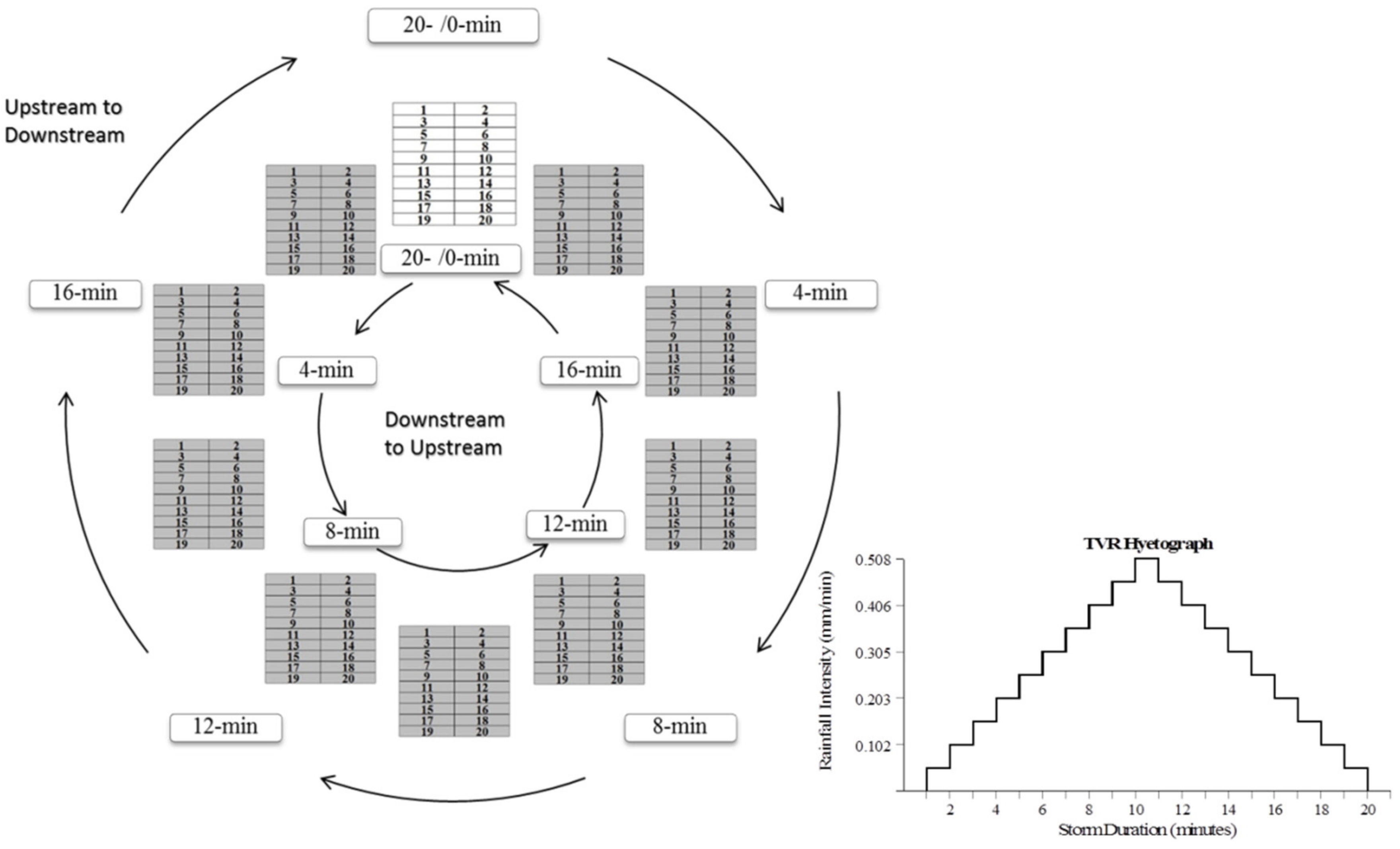
To imitate rainfall input to lumped hydrologic models, temporally varied rainfall, henceforth referred to as TVR, is derived to keep the following features identical with those of the moving storm: duration, total depth, and incremental mean areal precipitation (MAP) over the drainage basin. TVR is applied to each hydrologic model by spatially-averaging the corresponding SVR event and uniformly applying it to all areal units at each time step. This results in a uniform precipitation field which initially increases in rainfall intensity, with the peak intensity occurring at the middle time step, then decreasing thereafter. The total volume, depth and duration of rainfall of TVR remain unchanged as those of SVR.
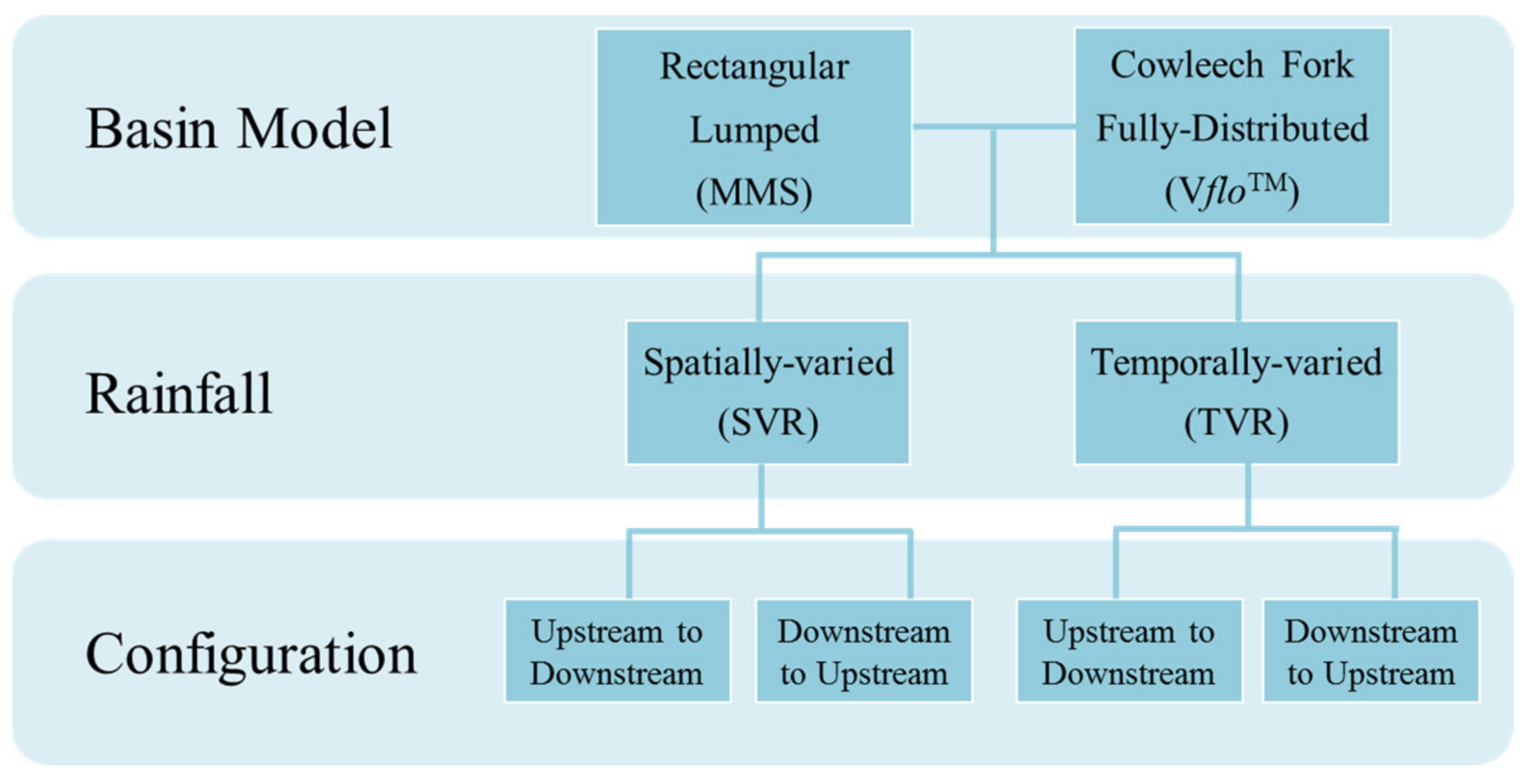
Two sets of experimental watersheds are established to receive the synthetic rainfall and simulate runoff. First, synthetic rectangular drainage basins with various shapes are created with the USGS Modular Modeling System (MMS) which includes the Precipitation-Runoff Modeling System (PRMS) module [41,42]. Second, to best represent the real world conditions, the Cowleech Fork watershed, located near Greenville, Texas, is selected to be modeled with VfloTM, a fully-distributed hydrologic model, which can precisely represent the spatial distribution of soil properties and produce physically realistic hydrologic simulations for both urban and rural watersheds [43]. The created VfloTM model further undergoes calibrations to ensure its accuracy. Overall, these two watersheds follow a progressive rationale, where complex from realistic assumptions was sequentially added into the experiments. Theoretical assumptions are made for the first scenario to investigate the effects and sensitivities of various factors in rainfall and catchments, while the second scenario best represents the realistic watershed condition. The general workflow of the study is shown in Figure 1 with two scenarios as listed below:
Scenario 1: SVR and TVR applied to synthetic rectangular drainage basins with impervious conditions using a lumped model (Modular Modeling System);
Scenario 2: SVR and TVR applied to an actual drainage basin using fully-distributed model (VfloTM).
2.1. Synthetic Rectangular Drainage Basins
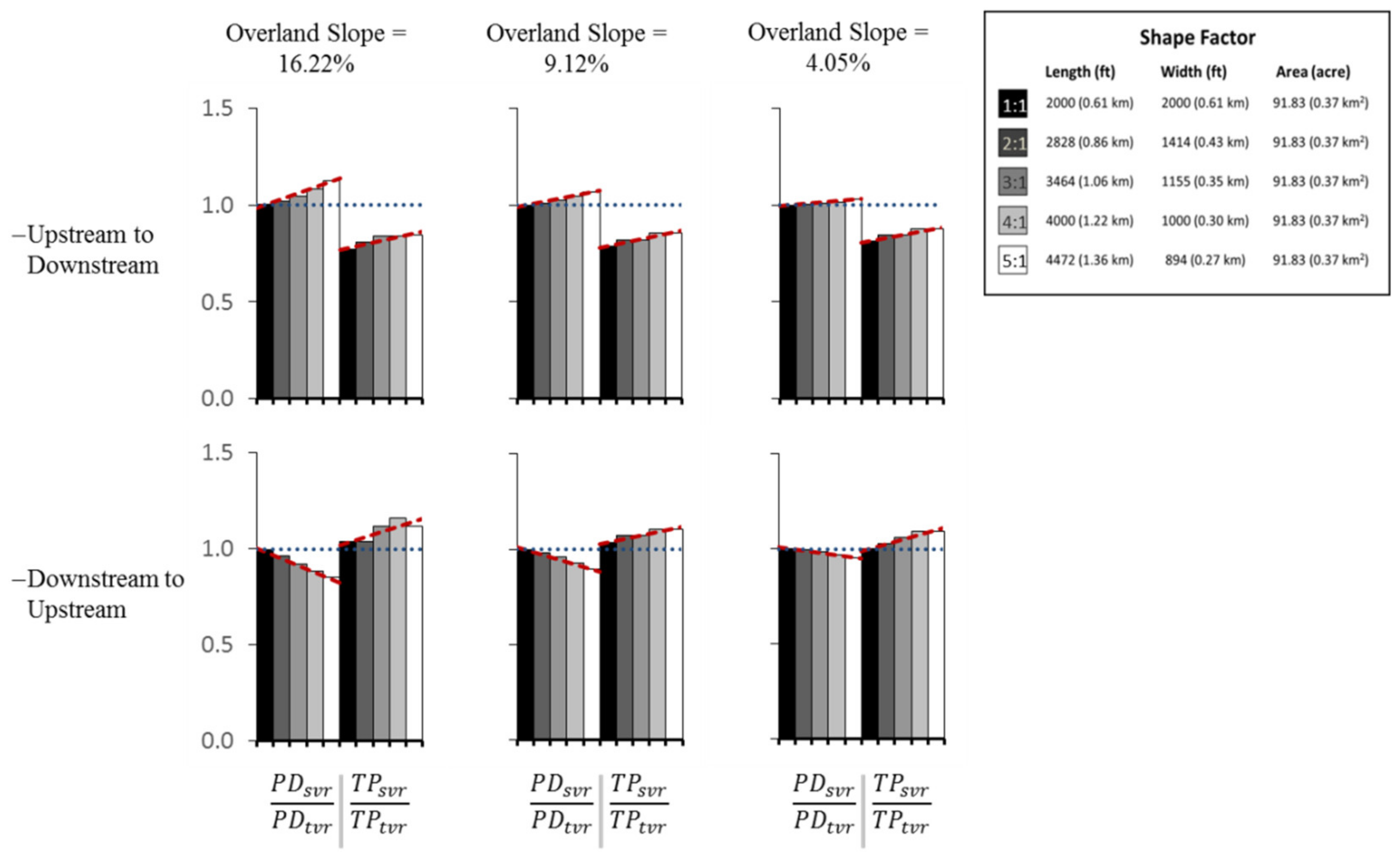
To evaluate the spatiotemporal characteristics of moving storms, a series of simple rectangular basin models are developed according to shape factors using MMS, as shown in Table 1.
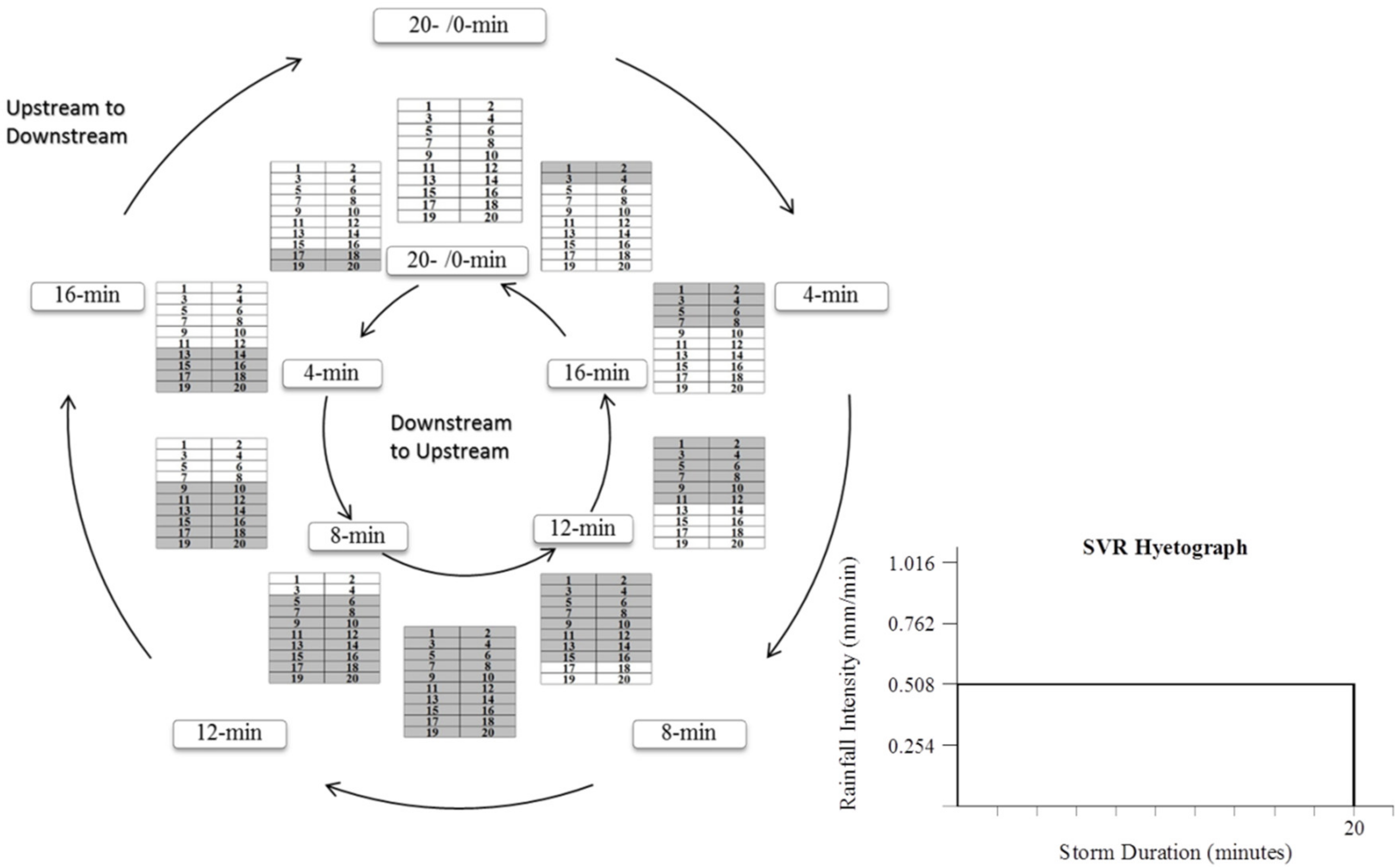
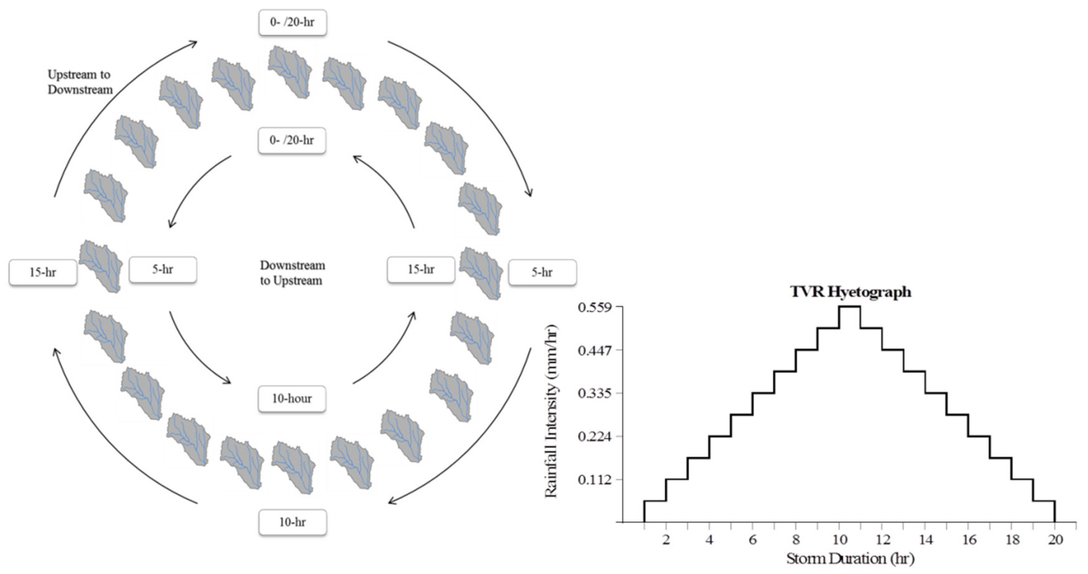
The shape factor refers to the length-to-width ratio and the areas of synthetic rectangular basins are kept constant. These V-shaped synthetic rectangular basins are bisected in half along their lengths by a major drainage channel, creating two overland flow planes. The two planes are then subdivided further into 10 identical sections along the length, creating a total of 20 overland flow planes. The basins are assumed to be impervious to eliminate the role of infiltration parameters and other watershed characteristics. Any changes in model output can therefore be directly associated with the location, intensity and movement of the simulated rainfall. SVR and TVR scenarios are applied to each basin using a hypothetical rainfall amount of 5.08 mm (0.2 in) distributed over 10 equal areal units. The amount of rainfall is approximately equivalent to a two-year 10 min storm as outlined in NOAA Technical Memorandum NWS HYDRO-35 [44]. Rainfall is incrementally applied over a 20-min time period in 1-min intervals as the hypothetical moving storm travels either (1) UtoD or (2) DtoU. SVR represents the spatially-distributed features of a synthetic storm moving across a watershed by incrementally applying rainfall from one end of the watershed to the other. In other words, SVR demonstrates a real representation of a moving storm across the watershed with constant rainfall intensity (0.508 mm/min). To achieve this goal, an algorithm is developed to manage the allocations of rainfall (0.508 mm/min) to corresponding sub-basins along the moving directions (UtoD and DtoU) over the entire basin within a span of 20 min. For the UtoD SVR scenario, one can see that the algorithm manages to cover the eight upstream sub-basins (1–8), sixteen upstream sub-basins (1–16), twenty sub-basins (1–20), sixteen downstream sub-basins (5–20), eight downstream sub-basins (13–20), and no sub-basins with the rainfall intensity of 0.508 mm/min for the first four minutes, eight minutes, ten minutes, twelves minutes, sixteen minutes, and twenty minutes, respectively. Figure 2 shows the temporal change of the actual location in which SVR is placed over the basins, with the clock-wise arrow indicating the UtoD configuration and the counter-clockwise arrow for the DtoU configuration. The storm movement can be found to cover the whole watershed at half the duration and completely exit at the end. Identically for both configurations, the hyetograph on the right shows the rainfall intensity where SVR is placed, instead of the areal averaged rainfall intensity over the whole watershed. Similarly, the scenarios of the corresponding TVR crossing the whole watershed for both moving configurations are shown in Figure 3. TVR is generated by areal averaging the same amount rainfall as SVR for each time step over the entire basin. TVR covers the whole basin but with different rainfall intensity for each time step. The rectangular hyetographs for SVR and the triangular hyetographs for TVR are input to the twenty sub-basins for further simulation in the MMS. The rainfall amount and duration are held constant in both TVR and SVR.
Each rectangular basin is designed to represent flow planes with varying slopes. The kinematic wave technique, based on three kinematic alpha parameters, that is, 4, 3, and 2, are used to compute three overland slopes, that is, 16.22%, 9.12%, and 4.05%. A slope of 1.55 % is used for the channel to represent typical slopes of north central Texas. It should be noted that the physical properties of the kinematic wave technique do not allow for the attenuation of the flood wave [45,46,47,48,49,50,51,52,53,54,55]. Manning’s n roughness coefficients are selected based on typical roughness factors associated with drainage areas located in North Central Texas. A Manning’s n coefficient of 0.15 is selected to represent tall grass vegetation for the overland flow planes. A Manning’s n coefficient of 0.05 is selected to represent the main stream channel in its natural condition [56].
2.2. Actual Drainage Basin
2.2.1. Study Area
Cowleech Fork of the Sabine River (Cowleech Fork) basin is selected as an actual basin for the second scenario. The basin is composed of two 12-Digit Hydrologic Unit Codes (HUCs), including Horse Creek (120100010103) and Hickory Creek (120100010102) of the Cowleech Fork Sabine River located near Greenville, Texas, approximately 80 km (50 mi) northeast of Dallas. The topography of this basin is generally flat with some rolling hills with an average elevation of 164 m. Greenville receives approximately 110 cm of rainfall annually, characterized by occasional heavy rainfall for brief periods of time and thunderstorm activities most common in the spring. The largest portion of the annual precipitation results from thunderstorm activity. The vegetation cover consists of primarily timber, shrubs, and grasses with the soil type defined as mostly clay. Cowleech Fork is somewhat rectangular in shape with an average length-to-width ratio of approximately 2.75 and the overland slopes range from approximately 1% to 4%.
2.2.2. Model Development
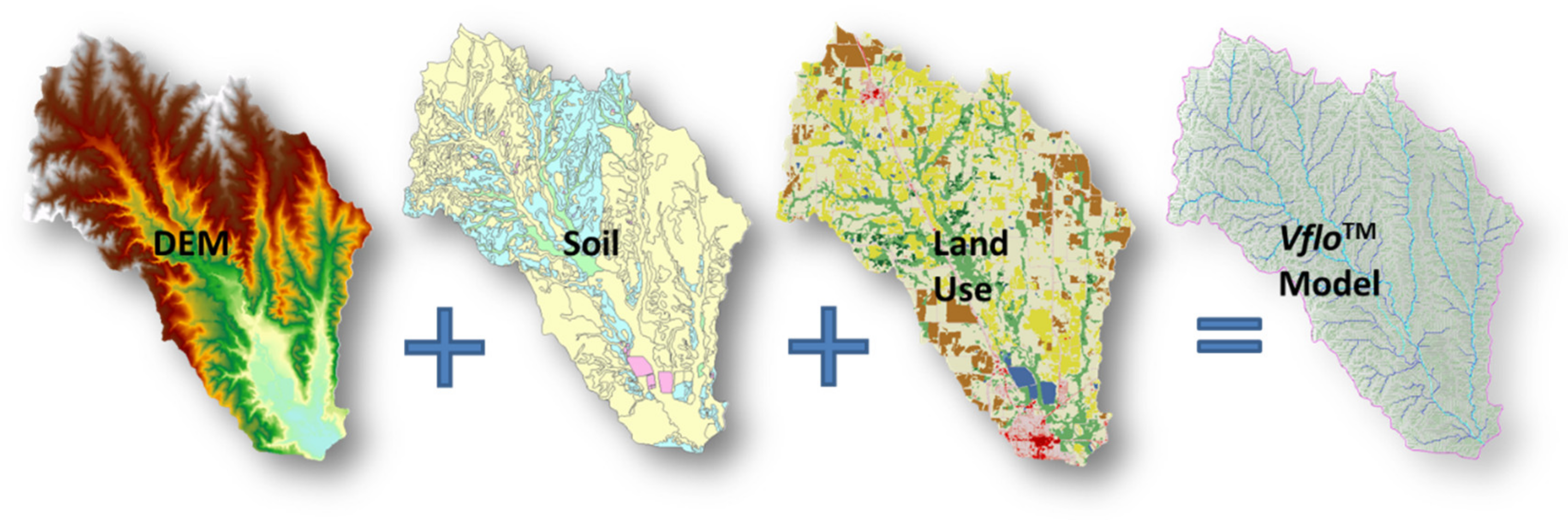
A distributed hydrologic model, VfloTM is developed for Cowleech Fork. VfloTM is a fully-distributed, physics-based model that rasterizes the study area with user-defined resolution and considers each cell as a single subcatchment [43]. Input data required for VfloTM model development includes Digital Elevation Model (DEM), land use information and soil parameters in the Green & Ampt infiltration method, which needs to be parameterized via ArcGIS. The 10-m resolution DEM is downloaded from USGS database (https://earthexplorer.usgs.gov). The land use information is obtained from the National Land Cover Database (https://www.mrlc.gov/nlcd2011.php) and the soil classification is from the Soil Survey Geographic Database (http://websoilsurvey.nrcs.usda.gov). Manning’s roughness are assigned based on predominate vegetation types across the study area. A Manning’s n value of 0.6 is used for timbered areas with moderately dense under brush, 0.4 for shrubs, and 0.13 for bare soil conditions. A Manning’s n value of 0.07 is selected for the river segments based on natural river channel conditions [56]. After processing required information in DEM, soil, and land use, one can see a generated VfloTM model as appeared in Figure 4. Cowleech Fork drains approximately 210 km2 (81 mi2) of area, represented by 20,979 grid cells in VfloTM using 100-m resolution.
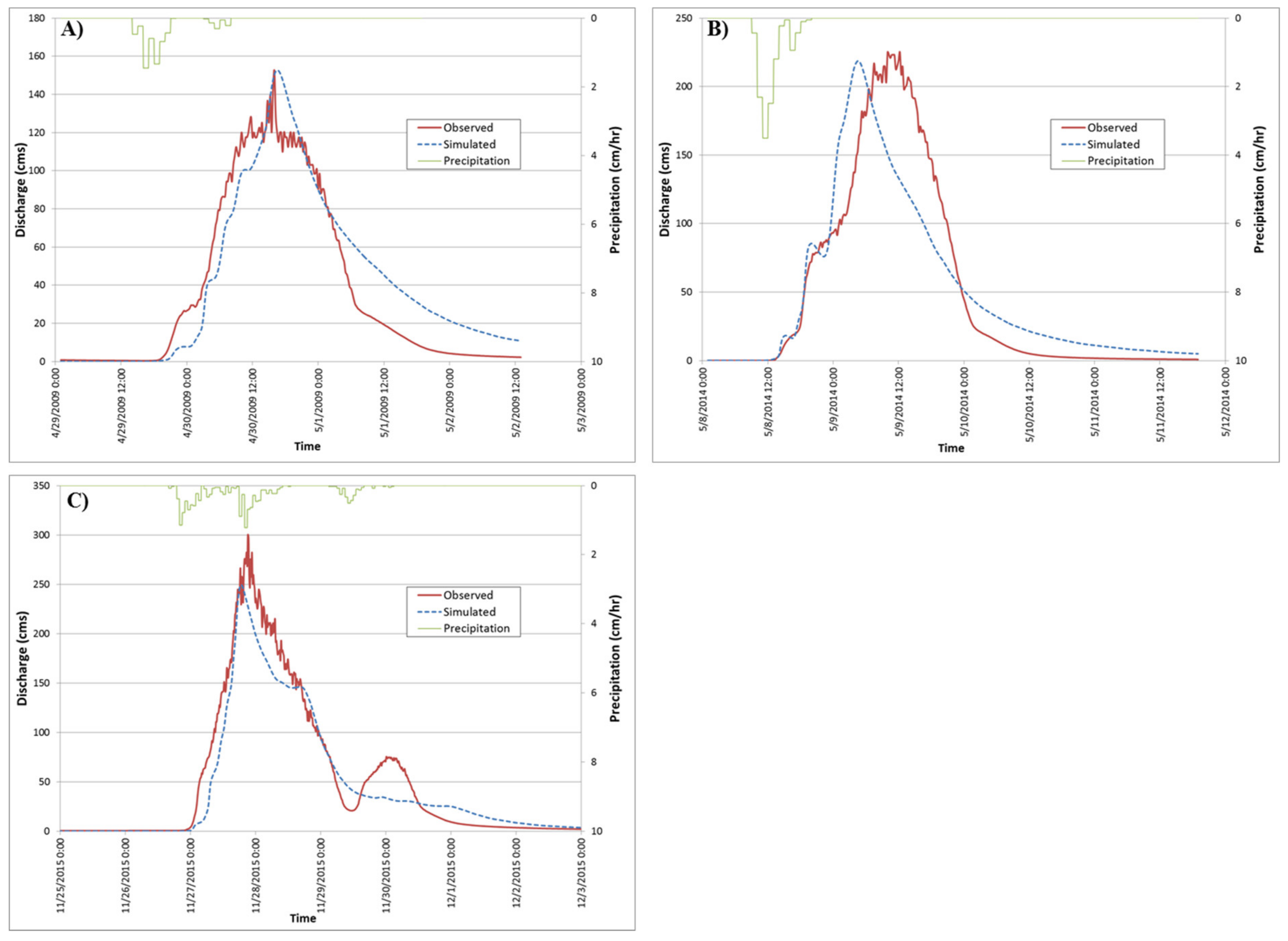
The model is then calibrated as described in Section 2.2.3 using NEXRAD radar rainfall data and the observed streamflow from a USGS Gage (8017200) of three storm events in April 2009, May 2014 and November 2015. The April 2009 event yields 8.8 cm (3.5 in) of rain within 24 h; the May 2014 event yields 15.0 cm (5.9 in) of rainfall within 24 h, and the November 2015 event yields 17.9 cm (7.0 in) rainfall in 48 h.
2.2.3. Model Calibration
Calibration of the VfloTM model is conducted by adjusting infiltration parameters including initial saturation, wetting front and hydraulic conductivity as well as channel and overland roughness. The VfloTM model can be adjusted for certain selected cells or a particular group of cells based on its fully-distributed features. As each parameter influences the discharge of the corresponding hydrograph differently, overall calibration efforts first focused on balancing the runoff volume by adjusting infiltration parameters. The channel roughness is calibrated next, which had a significant influence on peak timing and peak discharge. Finally, overland roughness is adjusted to fine-tune the model. Figure 5 shows the calibrated and observed hydrographs at the watershed outlet for the three storms in April 2009, May 2014 and November 2015 (also summarized in Table 2).
It is found that the simulated peak flow for the April 2009 event matches the observed, but the total volume differs by 13%. The difference in peak timing between simulated and observed is only 0.5-h. For the May 2014 event, the simulated peak flow is only 2% less than the observed while the total volumes matched very well with a peak timing difference of 6-h. The simulated peak discharge is 17% less than the observed peak discharge and the volume differs by 12% for the November 2015 event, while the rising limb matched well. The root-mean square error (RMSE) and Nash-Sutcliffe efficiency (NSE) values are shown in Table 2. Overall, the peak discharge and volume of the simulated hydrograph matches the observed adequately enough to serve as a good platform for the authors to apply moving storm features.
2.2.4. VfloTM Moving Storm Development
Prior to performing the moving storm simulation over Cowleech Fork in VfloTM, a time series of incremental rainfall raster datasets are developed as the input to the VfloTM model using the same geographic coordinate system as the Cowleech Fork watershed. The rainfall frequency Atlas of the United States, NOAA Technical Paper No. 40, is used as a guide to construct design storms using a rainfall amount which is smaller than 2-year storm thus occurs quite frequently over North Texas [57]. Table 3 summarizes the parameters that formulate the SVR configurations, including (1) UtoD and (2) DtoU.
The synthetic moving storm features a moving ‘frontal line’ separating the domain into a wet zone (behind the line) and a dry zone (in front of the line) at each time step. The wet zone is also constrained by storm size (Ls) while precipitation only occurs within a distance of Ls after the frontal line. Additionally, precipitation is assumed to be spatially uniform and temporally constant in the wet zone and the storm movement is assumed to be a straight line with constant velocity. The moving storm has the same length (Ls) as the watershed in the storm moving direction, which is the assumption used in the aforementioned scenarios for the synthetic catchments. The frontal line is initially tangential with the watershed boundary and is then moved for twice the distance of Ls. Based on the storm movement and the parameters in Table 3, each pixel value in the rainfall raster files is digitized accordingly. On the other hand, TVR is established to keep the following features identical with those of SVR: duration, total depth, and incremental mean areal precipitation (MAP) over the watershed. Unlike the SVR, TVR is spatially distributed over the whole drainage basin at each time step. Figure 6 and Figure 7 show the temporal change of the basins that receive rainfall and their corresponding hyetograph as results from the UtoD and DtoU storm movements, for SVR and TVR respectively.
3. Results and Discussion
Hydrologic simulations using both SVR and TVR are generated for (1) synthetic rectangular basins with impervious condition using a lumped model, (2) an actual river drainage basin, Cowleech Fork using a fully-distributed model. The comparison of simulation results using hydrologic models of increasing complexity thus allows for common paradigms of the modeling process to be revealed. For both SVR and TVR scenarios, the peak discharge (PD) and time-to-peak (TP) values are identified and recorded from the simulated hydrograph at the basin outlet. To aid in the comparison of SVR versus TVR, peak discharge ratios (PDR) and time-to-peak ratios (TPR) of SVR-divided-by-TVR are further computed using Equations (1) and (2), respectively:
A value equal to 1.0 of PDR and TPR indicates that there is no difference in the peak discharge/time-to-peak value when the rainfall input is SVR or TVR. Consequently, a PDR value greater/less than 1.0 indicates that the SVR generated higher/lower peak discharge than TVR. A TPR value greater/less than 1.0 indicates that SVR generates slower/earlier time-to-peak than less TVR.
General results, irrespective of the basin model, indicate that the peak discharge is greater for storm systems moving UtoD when compared to identical storms moving in the opposite direction. Secondly, UtoD moving storms tend to yield higher peak flows for SVR when compared to TVR while the DtoU moving storms generate slightly lower peak flows for SVR than TVR. Finally, the UtoD moving storms (SVR) tend to generate an earlier time-to-peak value than both the DtoU moving storm and the equivalent TVR at the basin outlet.
3.1. Synthetic Rectangular Drainage Basins
The results for the synthetic rectangular basins are shown Figure 8. For storm systems moving UtoD, PDRs are generally greater than 1.0 and TPRs are less than 1.0. For storm systems moving the opposite direction (DtoU), PDRs are generally less than 1.0 and TPRs are larger than 1.0. Thus the storm moving UtoD tends to yield higher peak flows and earlier time-to peak for SVR when compared to TVR while storm moving DtoU tends to yield lower peak flows and slower time-to-peak for SVR than TVR.
It should be noted that shape factor (length vs. width) can also impact the magnitude of PDR and TPR. For storm moving UtoD, PDRs and TPRs increase as the shape factor increases. For storm moving DtoU, PDRs decrease while TPRs increase as the shape factor increases. In addition, the overland slope can also impact the PDR and TPR. From Figure 8, it can be seen that PDRs increase for UtoD and decrease for DtoU as the slope increases. It can be concluded that the differences of PDRs and TPRs both UtoD and DtoU increase as the shape factor (length-to-width ratio) and overland slope increase.
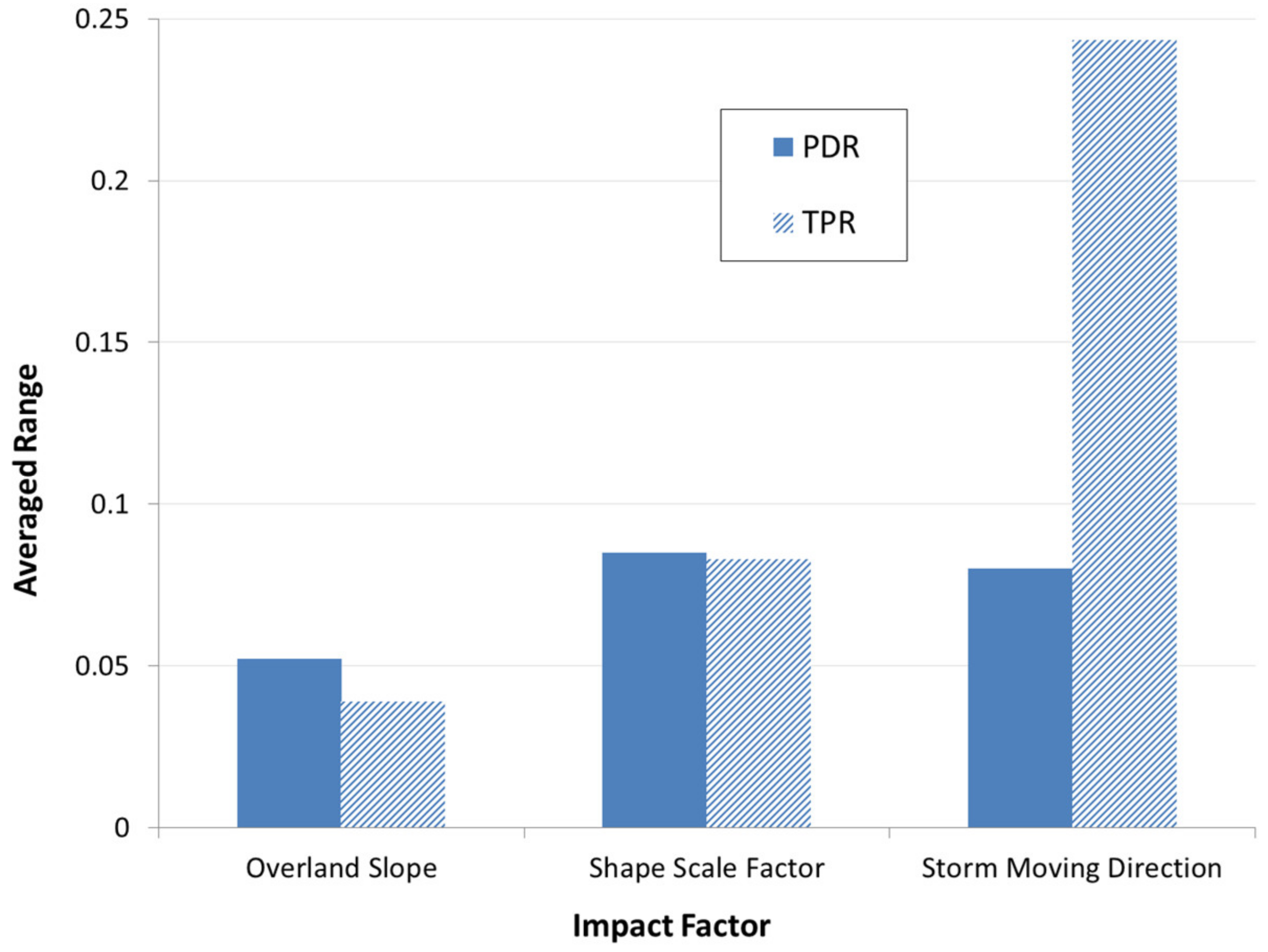
To better summarize the results, the change of PDR and TPR due to the three factors (storm moving direction, shape factor, and slope) is quantified via range i.e., maximum minus minimum. For each factor, the whole population of PDR or TPR values is divided into smaller samples. For instance, the total of 60 PDR values can be divided into 12 samples, each containing values from 5 different slopes. The range values calculated from each sample are then averaged to represent change due to the factor. As shown in Figure 9, the storm moving direction and slope have equally high impact on PDR, while TPR is most sensitive to change in storm moving direction. Therefore with considering of the overall effects on flood peaks, storm moving direction is regarded as the most influential factor and thus further investigated using the real basin as detailed in the following section.
3.2. Actual Drainage Basin
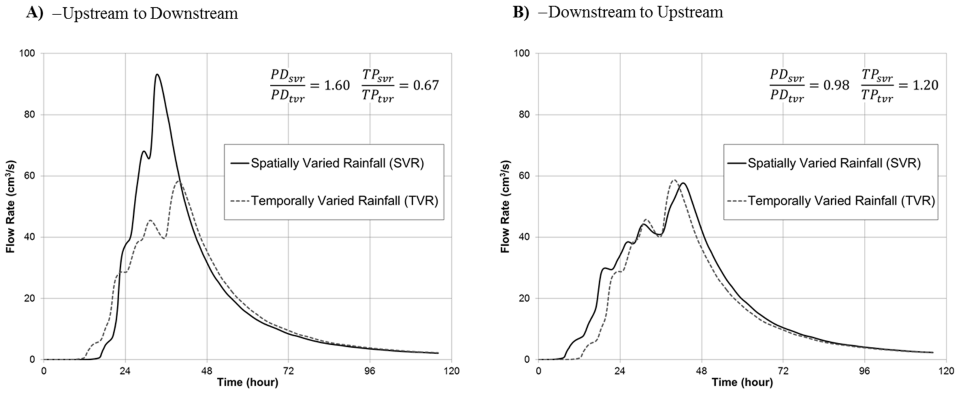
The corresponding hydrographs using SVR and TVR over the actual basin are shown in Figure 10A,B. Table 4 summarizes the comparison of these hydrographs in detail. First, one can see that the storm system (SVR) moving UtoD generates a significantly higher peak flow rate than the opposite moving storm despite identical net rainfall amounts; this finding is consistent with the results from the scenarios using synthetic rectangular basins. Second, the TVR scenarios yield a lower and a slightly higher peak flow rate than the moving storms for UtoD and DtoU configurations, respectively, which is again consistent with the findings from the scenarios using synthetic rectangular basin. Due to the larger coverage area of the TVR scenario, infiltration occurs at the basin-wide scale, leading to a higher portion of infiltrated rainfall, as shown in Table 4. Hence, one would expect an even smaller PDR for DtoU scenario if the natural basin were modeled under the conditions with impervious with no infiltration. Third, the UtoD moving storm (SVR) generates an earlier time-to-peak value than the equivalent TVR, while the DtoU moving storm (SVR) generates a slightly later time-to-peak than the TVR; these two findings again coincide with those from using synthetic rectangular basins.
4. Conclusions and Future Work
The insight from this study is obtained on the premise that distributed models are superior to lumped models in terms of representing the dynamic features of rainfall. As a unique contribution, this study enables us to separate the hydrologic effect of rainfall representation from those of other contributing factors, e.g., model parameters, model framework, etc., in the comparison of lumped and distributed hydrologic models. The study focuses on the hydrologic responses from the different rainfall representations in lumped and distributed models. The concepts of spatially varied rainfall (SVR) and temporally varied rainfall (TVR) are introduced to explore the advantages of distributed models over the lumped models. SVR is treated as the best attempt to capture the spatially-distributed features of a hypothetical moving storm while TVR serves to represent a simplified model commensurate with the mean areal characteristics of lumped modeling. As quantified by PDR and TPR, the distinction in hydrologic responses from SVR and TVR varies with storm moving directions and catchment characteristics. The following findings are reached about the hydrologic responses from the areal-averaging of rainfall:
In comparison of the simulated results from the distributed model using SVR, the areal-averaging of rainfall as a simplified approach to allocate rainfall information into a lumped model, can result in comparable peak values as long as overland slope of watershed is mild and shape of watershed is concentrated. When overland slope gets steeper and watershed shape gets more elongated, TVR will result in underestimated and delayed flood peaks.
The areal-averaging of rainfall causes most uncertainty in the simulated runoff when storms move from upstream to downstream, in which the peak discharge gets underestimated and peak timing gets delayed. When storms move from downstream to upstream, the TVR can result in comparable peak values as those using SVR.
As infiltration is involved in any real watershed, the areal-averaging of rainfall causes the infiltrated volume to be overestimated and thus the net runoff and peak discharge to be underestimated.
The knowledge gained from this study suggests that during hydrologic simulations, the distributed and lumped models respond to rainfall information differently. The understanding of the difference becomes more important especially when the spatiotemporal characteristics of moving storms need to be fully taken into account for hydrologic simulations. For future research, additional research effort is being invested to further enhance the capabilities of distributed hydrologic modeling. Forthcoming papers will present the comparisons of distributed and lumped models (SVR versus TVR) for basins with a constant overland flow slope with varying channel slopes. With the improved understanding on storm movement and its hydrologic impacts, the authors will investigate implementing the dynamic moving features of storms into engineering design practices in a future study. Additionally, future research will consider explicitly investigating the relationships between storm track direction, translational speed, and rainfall intensity characteristics (e.g., intensity, duration).
Author Contributions
All authors have contributed extensively to the work presented in this manuscript. Z.N.F, M.J.S., K.J.W. designed the methodology and Z.N.F. guided the research. K.J.W. organized figures and tables. Z.N.F., M.J.S. and K.J.W. prepared the original draft. J.Z. and S.G. calibrated and conducted the distributed model simulation. S.G. generated moving storm inputs for distributed model. J.Z. and S.G. carried out the analysis with the guidance of Z.N.F. All authors discussed the results and implications, and contributed to manuscript preparation/modifications. Z.N.F., J.Z. and S.G. discussed and contributed to the revised version. All authors read and approved the final manuscript.
Funding
This research received no external funding.
Acknowledgements
The authors are very grateful to Baxter Vieux and Vieux & Associates, Inc. for providing VfloTM software for the research.
Conflicts of Interest
The authors declare no conflict of interest.
References
- Rossman, L.A.; Dickinson, R.E.; Schade, T.; Chan, C.C.; Burgess, E.; Sullivan, D.; Lai, F.H. SWMM 5—The next generation of EPAs storm water management model. J. Water Manag. Model. 2004. [Google Scholar] [CrossRef]
- Vieux, B.E.; Moreda, F.G. Ordered physics-based parameter adjustment of a distributed model. Calibration Watershed Models 2003, 6, 267–281. [Google Scholar]
- Ogden, F.L.; Julien, P.Y. Runoff sensitivity to temporal and spatial rainfall variability at runoff plane and small basin scales. Water Resour. Res. 1993, 29, 2589–2597. [Google Scholar] [CrossRef]
- Refsgaard, J.C.; Knudsen, J. Operational validation and intercomparison of different types of hydrological models. Water Resour. Res. 1996, 32, 2189–2202. [Google Scholar] [CrossRef]
- Shultz, M.J.; Corby, R.J. Development, calibration, and implementation of a distributed model for use in real-time river forecasting. In Proceedings of the 3rd Federal Interagency Hydrologic Modeling Conference, Reno, NV, USA, 2–6 April 2006. [Google Scholar]
- Shultz, M.J.; Corby, R.J. Development, calibration, and implementation of a distributed hydrologic model for drainage basins located along the Texas Gulf Coast for use in real-time river flood forecast operations. In Coastal Hydrology and Processes: Proceedings of the AIH 25th Anniversary Meeting & International Conference “Challenges in Coastal Hyrology and Water Quality”, Baton Rouge, LA, USA, 21–24 May 2006; Singh, V.P., Xu, Y.J., Eds.; Water Resources Publications: Highland Ranch, CO, USA.
- Singh, V.P. Effect of spatial and temporal variability in rainfall and watershed characteristics on stream flow hydrograph. Hydrol. Process. 1997, 11, 1649–1669. [Google Scholar] [CrossRef]
- Gao, S.; Fang, Z. Using storm transposition to investigate the relationships between hydrologic responses and spatial moments of catchment rainfall. Nat. Hazards Rev. 2018, 19, 04018015. [Google Scholar] [CrossRef]
- Yen, B.C.; Chow, V.T. A laboratory study of surface runoff due to moving rainstorms. Water Resour. Res. 1969, 5, 989–1006. [Google Scholar] [CrossRef]
- Surkan, A.J. Simulation of storm velocity effects on flow from distributed channel networks. Water Resour. Res. 1974, 10, 1149–1160. [Google Scholar] [CrossRef]
- Ogden, F.L.; Richardson, J.R.; Julien, P.Y. Similarity in catchment response: 2. Moving rainstorms. Water Resour. Res. 1995, 31, 1543–1547. [Google Scholar] [CrossRef]
- De Lima, J.L.M.P.; Singh, V.P. The influence of the pattern of moving rainstorms on overland flow. Adv. Water Resour. 2002, 25, 817–828. [Google Scholar] [CrossRef]
- Lee, K.T.; Huang, J.K. Effect of moving storms on attainment of equilibrium discharge. Hydrol. Process. 2007, 21, 3357–3366. [Google Scholar] [CrossRef]
- Shah, S.M.S.; O’Connell, P.E.; Hosking, J.R.M. Modelling the effects of spatial variability in rainfall on catchment response—1. Formulation and calibration of a stochastic rainfall field model. J. Hydrol. 1996, 175, 67–88. [Google Scholar] [CrossRef]
- Johnson, D.L.; Miller, A.C. A spatially distributed hydrologic model utilizing raster data structures. Comput. Geosci. 1997, 23, 267–272. [Google Scholar] [CrossRef]
- Hydrologic Engineering Center (HEC). Hydrologic Modeling System HEC-HMS. Technical Reference Manual; U.S. Army Corps of Engineers: Davis, CA, USA, 2000.
- Reed, S.; Koren, V.; Smith, M.; Zhang, Z.; Moreda, F.; Seo, D.J. DMIP participants. Overall distributed model intercomparison project results. J. Hydrol. 2004, 298, 27–60. [Google Scholar] [CrossRef]
- Smith, M.B.; Seo, D.J.; Koren, V.I.; Reed, S.M.; Zhang, Z.; Duan, Q.; Moreda, F.; Cong, S. The distributed model intercomparison project (DMIP): Motivation and experiment design. J. Hydrol. 2004, 298, 4–26. [Google Scholar] [CrossRef]
- Wright, D.B.; Smith, J.A.; Baeck, M.L. Critical examination of area reduction factors. J. Hydrol. Eng. 2013, 19, 769–776. [Google Scholar] [CrossRef]
- Villarini, G.; Smith, J.A. Flood peak distributions for the eastern United States. Water Resour. Res. 2010, 46. [Google Scholar] [CrossRef]
- Knighton, J.; Steinschneider, S.; Walter, M.T. A vulnerability-based, bottom-up assessment of future riverine flood risk using a modified peaks-over-threshold approach and a physically based hydrologic model. Water Resour. Res. 2017, 53, 10043–10064. [Google Scholar] [CrossRef]
- Merz, B.; Aerts, J.C.J.H.; Arnbjerg-Nielsen, K.; Baldi, M.; Becker, A.; Bichet, A.; Delgado, J.M. Floods and climate: emerging perspectives for flood risk assessment and management. Nat. Hazards Earth Sys. Sci. 2014, 14, 1921–1942. [Google Scholar] [CrossRef]
- Shultz, M.J. Comparison of Distributed versus Lumped Hydrologic Simulation Models using Stationary and Moving Storm Events Applied to Small Synthetic Rectangular Basins and an Actual Watershed Basin. Ph.D. Thesis, Department of Civil Engineering, College of Engineering, University of Texas at Arlington, Arlington, TX, USA, 2007. [Google Scholar]
- Chappell, C.F. Quasi-stationary convective events. In Mesoscale Meteorology and Forecasting; Ray, P.S., Ed.; American Meteorological Society: Boston, MA, USA, 1986; pp. 289–310. [Google Scholar]
- Corfidi, S.F. Cold pools and MCS propagation: Forecasting the motion of downwind-developing MCSs. Weather Forecast. 2003, 18, 997–1017. [Google Scholar] [CrossRef]
- Schumacher, R.S.; Johnson, R.H. Organization and environmental properties of extreme-rain-producing mesoscale convective systems. Mon. Weather Rev. 2005, 133, 961–976. [Google Scholar] [CrossRef]
- Stephenson, D.; Meadows, M.E. Kinematic Hydrology and Modeling; Elsevier: New York, NY, USA, 1986. [Google Scholar]
- Viglione, A.; Chirico, G.B.; Woods, R.; Bloschl, G. Generalised synthesis of space-time variability in flood response—An analytical framework. J. Hydrol. 2010, 394, 198–212. [Google Scholar] [CrossRef]
- Seo, Y.; Schmidt, A.R.; Sivapalan, M. Effect of storm movement on flood peaks: Analysis framework based on characteristic timescales. Water Resour. Res. 2012, 48. [Google Scholar] [CrossRef]
- Story, G.J. Estimating precipitation from WSR-88D observations and rain gauge data. In Remote Sensing of Drought; Wardlow, B.D., Anderson, M.C., Verdin, J.P., Eds.; CRC Press/Taylor & Francis: Boco Raton, FL, USA, 2012; pp. 281–305. [Google Scholar]
- Bedient, P.B.; Holder, A.; Benavides, J.A.; Vieux, B.E. Radar-based flood warning system applied to Tropical Storm Allison. J. Hydrol. Eng. 2003, 8, 308–318. [Google Scholar] [CrossRef]
- Smith, J.A.; Baeck, M.L.; Meierdiercks, K.L.; Miller, A.J.; Krajewski, W.F. Radar rainfall estimation for flash flood forecasting in small urban watersheds. Adv. Water Resour. 2007, 30, 2087–2097. [Google Scholar] [CrossRef]
- Fang, Z.; Bedient, P.B.; Benavides, J.; Zimmer, A.L. Enhanced radar-based flood alert system and floodplain map library. J. Hydrol. Eng. 2008, 13, 926–938. [Google Scholar] [CrossRef]
- Fang, Z.; Bedient, P.B.; Buzcu-Guven, B. Long-term performance of a flood alert system and upgrade to FAS3: A Houston, Texas, Case Study. J. Hydrol. Eng. 2011, 16, 818–828. [Google Scholar] [CrossRef]
- Sharif, H.O.; Chintalapudi, S.; Hassan, A.A.; Xie, H.; Zeitler, J. Physically based hydrological modeling of the 2002 floods in San Antonio, Texas. J. Hydrol. Eng. 2011, 18, 228–236. [Google Scholar] [CrossRef]
- Looper, J.P.; Vieux, B.E. An assessment of distributed flash flood forecasting accuracy using radar and rain gauge input for a physics-based distributed hydrologic model. J. Hydrol. 2012, 412, 114–132. [Google Scholar] [CrossRef]
- Overeem, A.; Leijnse, H.; Uijlenhoet, R. Country-wide rainfall maps from cellular communication networks. PNAS 2013, 110, 2741–2745. [Google Scholar] [CrossRef]
- Carrera-Hernández, J.J.; Gaskin, S.J. Spatio temporal analysis of daily precipitation and temperature in the Basin of Mexico. J. Hydrol. 2007, 336, 231–249. [Google Scholar] [CrossRef]
- Lobligeois, F.; Andréassian, V.; Perrin, C.; Tabary, P.; Loumagne, C. When does higher spatial resolution rainfall information improve streamflow simulation? An evaluation using 3620 flood events. Hydrol. Earth Syst. Sci. 2014, 18, 575. [Google Scholar] [CrossRef]
- Ajami, N.K.; Gupta, H.; Wagener, T.; Sorooshian, S. Calibration of a semi-distributed hydrologic model for streamflow estimation along a river system. J. Hydrol. 2004, 298, 112–135. [Google Scholar] [CrossRef]
- Leavesley, G.H.; Lichty, R.W.; Troutman, B.M.; Saindon, L.G. Precipitation-runoff modeling system: User’s manual. Water-Resour. Investig. Rep. 1983, 83–4238. [Google Scholar] [CrossRef]
- Leavesley, G.H.; Restrepo, P.J.; Markstrom, S.L.; Dixon, M.; Stannard, L.G. The Modular Modeling System (MMS)—A Modeling Framework for Multidisciplinary Research and Operational Applications (User’s Manual); U.S. Geological Survey: Reston, WV, USA, 2004.
- Vieux, B.E.; Cui, Z.; Gaur, A. Evaluation of a physics-based distributed hydrologic model for flood forecasting. J. Hydrol. 2004, 298, 155–177. [Google Scholar] [CrossRef]
- Five- to 60-Minute Precipitation Frequency for the Eastern and Central United State; NOAA Technical Memorandum NWS Hydro-35: Silver Spring, MD, USA, 1977.
- Overton, D.E.; Meadows, M.E. Stormwater Modeling; Academic Press: New York, NY, USA, 1976. [Google Scholar]
- Ponce, V.M.; Li, R.M.; Simons, D.B. Applicability of kinematic and diffusion models. J. Hydraul. Division. 1978, 104, 353–360. [Google Scholar]
- MacArthur, R.C.; DeVries, J.J. Introduction and Application of Kinematic Wave Routing Techniques Using HEC-1; U.S. Army Corps of Engineers: Davis, CA, USA, 1979. [Google Scholar]
- Strelkoff, T. Comparative Analysis of Flood Routing Methods; U.S. Army Corps of Engineers: Davis, CA, USA, 1980. [Google Scholar]
- Choi, G.W.; Kang, K.W. Application of the generalized channel routing model. In Hydraulic Engineering, Proceedings of the 1990 National Conference sponsored by the Hydraulics Division of the American Society of Civil Engineers, San Diego, CA, USA, 1990; Volume 1. [Google Scholar]
- Ponce, V.M. The kinematic wave controversy. J. Hydraul. Eng. 1991, 117, 511–525. [Google Scholar] [CrossRef]
- Shultz, M.J. Comparison of Flood Routing Methods for a Rapidly Rising Hydrograph Routed Through a Very Wide Channel. Master’s Thesis, Department of Civil Engineering, College of Engineering, University of Texas at Arlington, Arlington, TX, USA, 1992. [Google Scholar]
- Mays, L.W. Water Resources Handbook; McGraw-Hill, Inc.: New York, NY, USA, 1996. [Google Scholar]
- Singh, V.P. Kinematic Wave Modeling in Water Resources; John Wiley & Sons, Inc.: New York, NY, USA, 1996. [Google Scholar]
- Brunner, G.W. River Analysis System HEC-RAS, Hydraulic Reference Manual; U.S. Army Corps of Engineers: Davis, CA, USA, 2002.
- Watershed Modeling Training Notes; USGS National Training Center: Denver, CO, USA, 2004.
- U.S. Department of Transportation, Federal Highway Administration (FHWA). Urban Drainage Design Manual; CreateSpace Independent Publishing Platform: Scotts Valley, CA, USA, 2001.
- Hershfield, D.M. Rainfall Frequency Atlas of the United States for Durations from 30 Minutes to 24 Hours and Return Periods from 1 to 100 Years; U.S. Dept. of Commerce, Weather Bureau: Washington, DC, USA, 1961.
Figure 1.
Research investigation workflow.

Figure 2.
Spatially varied rainfall (SVR) applied to synthetic rectangular drainage basins.

Figure 3.
Temporally varied rainfall (TVR) applied to synthetic rectangular drainage basins (mean areal precipitation).
Figure 3.
Temporally varied rainfall (TVR) applied to synthetic rectangular drainage basins (mean areal precipitation).

Figure 4.
Cowleech Fork of the Sabine River, Texas—component data layers in VfloTM model.

Figure 5.
VfloTM model calibration results (A) May 2009, (B) May 2014, and (C) November 2015.

Figure 6.
Spatially varied rainfall (SVR) applied to Cowleech Fork of the Sabine River, Texas.

Figure 7.
Temporally varied rainfall (TVR) applied to Cowleech Fork of the Sabine River, Texas.

Figure 8.
Synthetic rectangular drainage basins of constant area for peak discharge ratios (PDRs) and time to peak ratios (TPRs).
Figure 8.
Synthetic rectangular drainage basins of constant area for peak discharge ratios (PDRs) and time to peak ratios (TPRs).

Figure 9.
The averaged range of PDRs and TPRs due to overland slope, shape scale factor and storm moving direction.
Figure 9.
The averaged range of PDRs and TPRs due to overland slope, shape scale factor and storm moving direction.

Figure 10.
Actual drainage basin, Cowleech Fork of the Sabine River Texas, fully-distributed model (VfloTM) using pervious conditions, hydrographs at drainage basin outlet for SVR and TVR for (A) UtoD and (B) DtoU scenarios.
Figure 10.
Actual drainage basin, Cowleech Fork of the Sabine River Texas, fully-distributed model (VfloTM) using pervious conditions, hydrographs at drainage basin outlet for SVR and TVR for (A) UtoD and (B) DtoU scenarios.


Table 1.
Rectangular basin dimensions and shape factor (length vs. width).
| Shape Factor | Length (m) | Width (m) | Area (km2) |
|---|---|---|---|
| 1 | 609.6 | 609.6 | 0.37 |
| 2 | 862 | 431 | 0.37 |
| 3 | 1055.8 | 355.4 | 0.37 |
| 4 | 1219.2 | 304.8 | 0.37 |
| 5 | 1363.1 | 272.5 | 0.37 |
Table 2.
VfloTM calibration summary.
| Event | ∆Peak | ∆Time (h) | ∆Vol | RMSE (m3/s) | NSE |
|---|---|---|---|---|---|
| 2009 May | 0% | 0.5 | 13% | 8.5 | 0.86 |
| 2014 May | −2% | −6 | 0% | 27.7 | 0.81 |
| 2015 November | −17% | 2.5 | −12% | 13.2 | 0.92 |
Table 3.
Parameter setup for the synthetic moving storm scenarios.
| Storm Size (km) | 25.09 |
|---|---|
| Rainfall Duration (h) | 20 |
| Rainfall Intensity (mm/h) | 5.6 |
| Storm Moving Direction (°) | 300 (120 *) |
| Storm Moving Velocity (km/h) | 2.51 |
* Storms move against the streamflow direction and the value is the counterclockwise angle from west-east direction.
Table 4.
Summary of hydrologic responses from SVR and TVR for UtoD and DtoU scenarios in Cowleech Fork watershed.
Table 4.
Summary of hydrologic responses from SVR and TVR for UtoD and DtoU scenarios in Cowleech Fork watershed.
| Hydrologic Responses | Upstream to Downstream | Downstream to Upstream | ||
|---|---|---|---|---|
| SVR | TVR | SVR | TVR | |
| Runoff Volume (mm) | 37 | 33 | 37 | 33 |
| Precip. Volume (mm) | 56 | 56 | 56 | 56 |
| Infiltrated Volume (mm) | 16 | 20 | 16 | 20 |
| Peak Discharge (m3/s) | 93 | 58 | 58 | 59 |
© 2019 by the authors. Licensee MDPI, Basel, Switzerland. This article is an open access article distributed under the terms and conditions of the Creative Commons Attribution (CC BY) license (http://creativecommons.org/licenses/by/4.0/).
Share and Cite
MDPI and ACS Style
Fang, Z.N.; Shultz, M.J.; Wienhold, K.J.; Zhang, J.; Gao, S. Case Study: Comparative Analysis of Hydrologic Simulations with Areal-Averaging of Moving Rainfall. Hydrology 2019, 6, 12. https://doi.org/10.3390/hydrology6010012
AMA Style
Fang ZN, Shultz MJ, Wienhold KJ, Zhang J, Gao S. Case Study: Comparative Analysis of Hydrologic Simulations with Areal-Averaging of Moving Rainfall. Hydrology. 2019; 6(1):12. https://doi.org/10.3390/hydrology6010012
Chicago/Turabian StyleFang, Zheng N., Michael J. Shultz, Kevin J. Wienhold, Jiaqi Zhang, and Shang Gao. 2019. "Case Study: Comparative Analysis of Hydrologic Simulations with Areal-Averaging of Moving Rainfall" Hydrology 6, no. 1: 12. https://doi.org/10.3390/hydrology6010012
Note that from the first issue of 2016, this journal uses article numbers instead of page numbers. See further details here.