Spatiotemporal Surface Moisture Variations on a Barred Beach and their Relationship with Groundwater Fluctuations

Abstract

Understanding the spatiotemporal variability of surface moisture on a beach is a necessity to develop a quantitatively accurate predictive model for aeolian sand transport from the beach into the foredune. Here, we analyze laser-derived surface moisture maps with a 1 × 1 m spatial and a 15-min temporal resolution and concurrent groundwater measurements collected during falling and rising tide at the barred Egmond beach, the Netherlands. Consistent with earlier studies, the maps show that the beach can be conceptualized into three surface moisture zones. First, the wet zone just above the low tide level: 18–25%; second, the intertidal zone: 5–25% with large fluctuations. In this zone, surface moisture can decrease with a rate varying between ∼2.5–4% per hour, and cumulatively with 16% during a single falling tide; and, third, the back beach zone: 3–7% (dry). The bar–trough system perturbs this overall zonation, with the moisture characteristics on the bar similar to the upper intertidal beach and the trough always remaining wet. Surface moisture fluctuations are strongly linked to the behavior of groundwater depth and can be described by a ’Van Genuchten-type’ retention curve without hysteresis effects. Applying the Van Genuchten relationship with measured groundwater data allows us to predict surface moisture maps. Results show that the predictions capture the overall surface moisture pattern reasonably well; however, alongshore variability in groundwater level should be improved to refine the predicted surface moisture maps, especially near the sandbar.

1. Introduction

Aeolian sand transport from the beach contributes to dune growth and recovery after erosion from storm-wave processes. Well-developed dune-erosion models (e.g., van Gent et al. [1], Roelvink et al. [2]) are already in use for scientific and applied studies. In contrast, dune-growth models driven by aeolian-process dynamics are less advanced and are generally conceptual [3]. However, recently introduced dune-growth models by Delgado-Fernandez [4], Keijsers et al. [5], and Hoonhout and De Vries [6] show promising results. Nonetheless, prediction of aeolian sediment transport remains unsolved at a variety of temporal and spatial scales. Predicted rates of sand flux or net deposition on the foredunes generally do not correspond well with observations [7,8,9]. Limiting factors of aeolian sand transport play an important role in solving and improving these predictions [10].

Surface moisture is often considered as a key supply-limiting factor. A higher surface moisture content increases the shear velocity threshold required to entrain sediment [11] and is therefore a primary control on the development of the fetch effect [4]; that is, saturated transport rates are not yet reached at the beach–dune interface. When surface moisture exceeds about 10% by mass, it prohibits aeolian sand transport entirely (e.g., Delgado-Fernandez [10]). On the whole, estimated transport equations that assume dry sand generally over-predict aeolian sand transport from the beach into the dunes. Considerable progress has been made in measuring the temporal and spatial variability in surface moisture in the intertidal zone and back beach area by using the optical brightness method [12,13], soil moisture probes [14,15,16] and a Terrestrial Laser Scanner (TLS) [17,18]. Especially the shortwave near-infrared TLS has shown success in measuring surface moisture content over its full range with a high spatiotemporal resolution [18], necessary to investigate the key processes that drive spatiotemporal surface moisture variations.

Previous studies (e.g., Namikas et al. [15], Yang and Davidson-Arnott [19], Bauer et al. [20], Schmutz and Namikas [21], Brakenhoff et al. [22]) have demonstrated that spatial surface moisture fluctuations on planar beaches can be conceptualized into three zones. From the sea towards the dunes, these three surface moisture zones are, firstly, the wet zone (just above the low-tide level) where gravimetric surface moisture ($w_s$) always exceeds 20% to 25%; secondly, the intertidal zone (middle to upper tidal zone) where $w_s=5\%-25\%$ and $w_s$ can vary strongly with time; and, thirdly, the dry zone (just above the high-tide level) where $w_s<5\%$ and temporal variations are low. The conceptualization of the beach into three surface moisture zones becomes more complex in the presence of a bar–trough system. Oblinger and Anthony [23] describe how surface moisture on a macro-tidal beach with multiple bars and troughs is strongly dependent on the cross-shore topographic variations induced by the bar-though couplets. The bars show low to moderate moisture content compared with the lower-lying troughs, with an overall seaward increase in moisture contents when moving further away from the dune foot.

Spatiotemporal surface moisture fluctuations ($w_s$) can be related to tide-induced groundwater fluctuations. Beach environments often have very shallow water table depths (centimeters to a few meters), and the influence of the groundwater table depth (h) on surface moisture is especially high in the wet- and intertidal zone of the beach [13,15,19,21,22]. Research by Atherton et al. [24] states that on a beach with relatively fine sand (D50 = 160 $\mathsf{\mu }$m) dewatering and drying of the beach during falling tide is less because of the thicker capillary fringe. Thus, even though h can increase to 0.4 m or more, the sand at the surface remains saturated and did not result in a discernible decline in surface moisture content ($w_s\sim$ 3.5%). However, Darke and McKenna Neuman [25] showed different results for non-tidal beaches (D50 = 200 $\mathsf{\mu }$m). Here, $w_s$ was saturated for $h<0.2$ m, with a drop in $w_s$ to near 0% with an increase in h to $0.4–0.5$ m depth. When $h>0.5$ m, $w_s$ was ∼0% and the relationship between h and $w_s$ diminished. Additionally, Schmutz and Namikas [26] looked at the relationship between $w_s$ and h in the laboratory with a vertical sand column (D50 = 130 $\mathsf{\mu }$m) and a varying groundwater table and showed that the relationship between $w_s$ and h is different for a rising water table than for a falling water table.

Accordingly, the connection between the groundwater table depth and soil moisture content can be explained by a soil water retention curve that describes at which suction rate water is hold by the soil particles and when water is drained to the groundwater table. The shape of the curve depends on the grain size of the soil and the magnitude of groundwater fluctuation [27,28]. As the elevation of the surface above the water table changes across the beach due to morphology and the tide-induced groundwater fluctuations, the intersection of the curve with the beach surface changes as well. The soil moisture retention curve is thus truncated at the pressure head elevation of the sediment surface layer [15]. When assuming a steady state at each stage of the moving groundwater table, the vertical moisture profile with an empirical soil water retention curve [29] can be used to link soil moisture at the surface to groundwater depth. Depending on the rate of rise or fall of the water table, the vertical moisture profile may be compressed or stretched out [15,30]. Schmutz and Namikas [21] found that, on a microtidal beach (130 $\mathsf{\mu }$m), hysteresis plays an important role. While Brakenhoff et al. [22] demonstrated with field experiments on a 365 $\mathsf{\mu }$m microtidal beach that surface moisture dries and continues doing this until the beach is inundated and it becomes saturated at once. They did not find wetting processes in front of the rising tide. This could imply that the influence of hysteresis diminishes with increasing grain size (e.g., [19,31]).

In the present paper, we extend previous work on surface moisture variability on coastal beaches by addressing this variability and its causes on a barred beach. The data include high-resolution (1 × 1 m) TLS derived surface moisture maps collected with a 15–30 min resolution at the microtidal barred beach of Egmond aan Zee, the Netherlands, and simultaneously collected groundwater levels with a 1-min resolution across the beach. With these data we aim, firstly, at analyzing spatiotemporal surface moisture variations during a tidal cycle; secondly, to link these variations to groundwater depth while considering the superimposed topography variations by the cross-shore migrating sandbar; and, thirdly, to address the suitability of predicting surface moisture maps from groundwater depth and the Van Genuchten [29] retention curve.

2. Methodology

2.1. Study Site

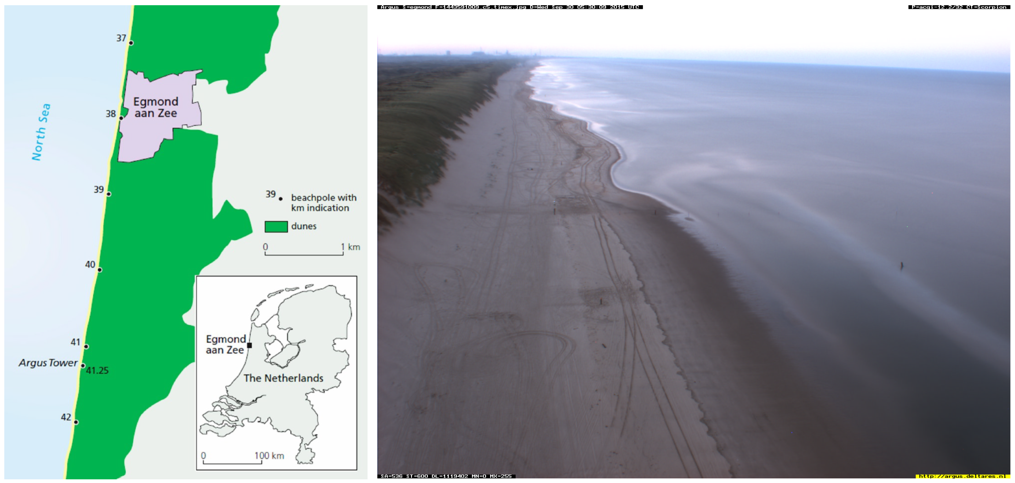
The spatial and temporal surface moisture variability as well as tidal seawater oscillations and groundwater fluctuations were measured during a six-week fieldwork campaign from 22 September until 30 October 2015 at the beach of Egmond aan Zee in the Netherlands. The study site is located on the roughly north–south oriented central Holland coast, which is approximately 120 km long (Figure 1). This micro- to meso-tidal site is dominated by waves that are generated on the North Sea. The beach comprises two subtidal sandbars [32], an intertidal slipface ridge [33], and is relatively narrow (∼100 m maximum at spring low tide) and mildly sloping (∼1:30). It consists predominantly of quartz sand with a median diameter of about 250 $\mathsf{\mu }$m. The foredune at Egmond aan Zee is largely covered by European Marram grass (Ammophila arenaria) and is ∼25 m high with a steep seaward facing slope because of occasional erosional events in winter (e.g., De Winter et al. [34]). Embryo dunes can develop on the upper beach in front of the foredune during years without any noteworthy storms and associated surges.

To gain more insight in the soil characteristics and grain size distribution over the vertical and horizontal plane of the beach, a total of nine soil moisture retention curves (pF-curves) were made in the Wageningen Soil Physics Laboratory from samples taken on 20 October 2015. Three soil samples were taken over different depths (top layer 0–6 cm, second layer 6–12 cm, third layer 12–18 cm) in three different beach zones, that is, in the swash near the low-tide level, on the intertidal beach and at the dune foot. A pF-curve was measured on intact soil cores using tension table and pressure plate methods [36]. All points on the pF-curve describe equilibrium situations between suction and moisture content. The suction is presented as pF, which is the logarithm of the suction in centimetres. Figure 2 shows that all pF-curves, despite being taken in different zones and over different depths, show minimal variation, implying that the soil has the same characteristics over depth and width of the beach. The soil reaches complete saturation with a volumetric value of ${\theta }_{sat}$ = 25%, while the residual volumetric moisture content ${\theta }_{res}$ = 3.5%, implying that the soil never dries out completely. The pF-curves also show a quick (horizontal) drop in moisture content at pF $=1.5$. Such a steep transition indicates that the grain size distribution is very well-sorted. This was confirmed by several sieve curves that were taken from the Egmond beach sand. Results show that the grain size distribution is well sorted over the entire beach with a D10 of 300–425 $\mathsf{\mu }$m, a D50 of 250–300 $\mathsf{\mu }$m and a D90 of 180–250 $\mathsf{\mu }$m.

2.2. Measurements

2.2.1. TLS-Based Surface Moisture

Measurements with a short-wave infrared (1550 nm) RIEGL VZ-400 Terrestrial Laser Scanner (TLS) (RIEGL, Horne, Austria) were performed on 29 September and 29 October, 2015 to quantify spatiotemporal surface moisture dynamics. These surveys inherently collect a 3D point cloud with positional ($x,y,z$) data and corresponding reflectance data. The TLS captured these data by operating in the panoramic scan mode. In a panoramic scan $\varphi$ (horizontal rotation) changes from 0${}^{\circ }$ to 360${}^{\circ }$, while for each $\varphi$, $\theta$ (vertical rotation) changes from its minimum 80${}^{\circ }$ to its maximum 130${}^{\circ }$. In the present work, the $\varphi$ step size was also 0.020${}^{\circ }$ and the $\theta$ step size was 0.020${}^{\circ }$, resulting in a typical scan duration of 12 min. Panoramic scans were repeated every 15 min and were performed from low tide towards high tide (11:00 a.m. to 6:00 p.m. on both days). A total of 41 surveys were performed during the two survey days. With the use of retro reflective cylinders with known coordinates, the ($x,y,z$) were converted into a local coordinate system, in which x and y are cross-shore and alongshore coordinates, respectively, and z is elevation with respect to Mean Sea Level (MSL).

Each 3D point cloud was processed into $1\times 1$ m grid cells by taking the median range-corrected reflectance T of each grid cell. This minimized instrument noise while retaining any true larger scale reflectance trends. Smit et al. [18] illustrated that T relates well to gravimetric surface moisture content $w_s$. Based on earlier results at Egmond aan Zee, Smit et al. [18] found the following relationship between $w_s$ and T,

$$\widetilde{w_s}\left(T\right)=\frac{w_{min}-w_{max}}{1+e^{-a(T-c)}}+w_{max},$$

(1)

where ∼ indicates a predicted value of w (surface moisture), $w_{max}=25\%$, $w_{min}=3\%$, $a=0.86$ and $c=-10.43$. The correlation-coefficient squared ($r^2$) of the curve amounted to 0.85 and the Root-Mean-Square Error (RMSE) was 2.69%. With this relationship, the T grids were converted into $w_s$ grids. In its present set-up, the height of the TLS is 1.86 m above beach level, which, as outlined in Smit et al. [18], implies that the calibration curve is applicable for distances between ∼20 m to 60 m from the TLS. An example of a TLS-derived surface moisture map is given in Figure 3.

2.2.2. Groundwater and Tidal Fluctuations

Groundwater table fluctuations were measured throughout the campaign with 10 pressure transducers placed inside wells arranged in a cross-shore array from the mean shoreline to the dune foot (Figure 3 and Figure 4). These wells are termed W1–W10 from sea to land in the following.

The sample frequency of each pressure transducer was $1/60$ Hz. The wells consisted of a steel tube of 2 to 4 m in length and 0.05 m in diameter, with a perforated lower end of approximately 1 m. In the steel tube, a PVC pipe was inserted, with a filter of 50 $\mathsf{\mu }$m at the lower end, to prevent the entering of sand. The height of the top of each well relative to Dutch Ordnance Datum (NAP; 0 m NAP is equal to Mean Sea Level, MSL) was determined several times with RTK-GPS with an accuracy of 0.02 m, and the individual heights were averaged. As the pressure transducers were at a known distance beneath the top of the well, the water level fluctuations are given with respect to MSL in the following. Initial inspection of the data revealed some sample-to-sample fluctuations of 0.05 m to 0.1 m when a well was submerged by the tide. These fluctuations are presumably wave-induced and were removed by filtering each series with a quadratic loess interpolator [37] with a scale factor $\lambda$ of 1 h. This interpolator acts as low-pass filter and removes variability at temporal scales of $\lambda /0.7$ (here, ∼1.4 h). Visual inspection of the filtered data revealed that this setting was effective in removing the rapid fluctuations while retaining the tidal signal.

About 41 m seaward of W1 an additional pressure transducer (PT) was deployed to measure tidal sea water fluctuations. For most of the time, it was submerged but sometimes during low tide it would fall dry. This pressure transducer operated at a sample frequency of 10 Hz. Because the pressure transducer collected at a higher interval than the groundwater pressure transducers, the instantaneous PT data were processed into 1-min average values (with respect to MSL), where each block of 1 min was centered around the sample moments of the groundwater transducers.

2.2.3. Additional Measurements

Changes in beach morphology and tidal oscillations influence groundwater fluctuations over a longer (days) and smaller (hours) time scale, respectively. To examine the influence of groundwater fluctuations on surface moisture on this longer time scale, additional surface moisture measurements were executed on 10 days (25 until 27 September, 1 and 2 October, and 20 until 24 October) with a Delta-T Theta probe (e.g., Schmutz and Namikas [14], Tsegaye et al. [38]) next to the 10 groundwater wells. The probe consists of four stainless steel pins. To ensure that the probe would specifically measure surface moisture, the length of each pin was shortened from 0.06 m to 0.02 m (e.g., Brakenhoff et al. [22]). Because the sand properties are constant, the probe can measure the relative change in surface moisture. To translate the dielectric output to a surface moisture content for the Egmond beach, a calibration curve was produced where probe measurements were related to gravimetric surface moisture samples (upper 2 cm). The dependence of the output of the probe was linearly related to moisture content, with a correlation coefficient squared $r^2$ of 0.96 and a standard error sE of 1.14%. On the stated days, probe measurements were performed during falling tide and rising tide; the specific time period and tidal elevation can be seen in Figure 5 in thick red lines. The time period and tidal conditions during TLS measurements are indicated in Figure 5 by thick blue lines.

2.3. Environmental Conditions

Figure 5 shows off shore water level oscillations, wave height (both measured by Rijkswaterstaat) and wind speed (measured by The Royal Netherlands Meteorological Institute, KNMI) during the entire campaign measured approximately 15 km south of the field site in IJmuiden. The campaign comprised two spring-neap tide cycles with water levels fluctuating over the range of ∼$-1$ to $+1.5$ m compared to MSL. During two moments, the 10-min. averaged wind speed (at 10 m height) exceeded 15 m/s (7 Beaufort). During the TLS and Delta-T theta probe measurements, this was not the case and aeolian activity was then absent. In addition, no rain fell during moisture measurements (not shown). Wave height correlates to wind speed with a maximum of 2.3 m on 22 October. On this day, the measured water level was somewhat above the astronomically predicted values, implying the presence of a small storm surge. On the whole, the conditions are mild with respect to the typical Dutch wind and wave climate. The mild character of the wave conditions is also reflected in the morphological evolution of the beach. During the campaign, one or two slip face ridges were generally present, which migrated onshore; see the example shown in Figure 4. These measurements were performed with an RTK-GPS mounted on a quad while driving two cross-shore transects along the groundwater wells within a time span of 15 min. Each transect indicated in Figure 4 represents the merged values of both transect. Figure 4a shows that on 25 September (yellow line) a single sandbar was present on the beach, while, on 26 and 27 September, two sandbars were present. Until 2 October, two sandbars of approximately 0.5 m high are clearly shown. One month later, between 20–24 October, a single sandbar was present moving landward with a steep slope facing the dune side and a more gentle slope towards the sea. The sandbar had a height above 1 m, which means that groundwater wells W1 to W4 were situated deeper compared to the beach surface. Over the entire campaign, sandbars were thus moving from the sea towards the dunes.

3. Results

3.1. Surface Moisture Dynamics

Figure 6 provides four surface moisture maps taken with a roughly 1.5–2 h interval during falling tide on 29 September 2015. The lighter yellow colors indicate low surface moisture content (<8%), which are visible on the back beach in front of the dunes ($z>1.15$ m). From the high water line in the seaward direction, the yellow colors descend into green, blue and darker blue colors, indicating higher surface moisture values. There is a steep incline in moisture content around the high water line ($x\sim -5$ m), as surface moisture in the intertidal zone varies from 10% surface moisture towards complete saturation of 25% near the waterline. In other words, the surface moisture maps clearly indicate that surface moisture increases towards the sea in the intertidal zone, but is constant and low on the upper beach. No data points are visible in the trough, as water here absorbs the laser pulse completely. In contrast, the sandbar seaward of the trough is drier than its surroundings, although it lies closer to the sea than the trough. Some unnatural features are visible such as tire tracks, which appear drier than their surroundings as well. The part within the circle around the TLS indicates the area of which Smit et al. [18] considered reflectance values to be less reliable; however, the surface moisture maps do not show deviating values in this area in our case.

Going from this general characterization of spatial surface moisture to more detailed dynamics during rising and falling tides, we next analyze cross-shore transects. Figure 7 shows cross-shore transects of median beach height (a and b) and surface moisture values over y for the same x-coordinate taken on 29 September and 29 October 2015 during falling (c and d) and rising tide (e and f), per half an hour and 15 min, respectively. Figure 7a,b) clearly show a sandbar–trough morphology. Surface moisture variations during falling tide (Figure 7c,d) above the high water line ($x\sim 0$ m) are minimal, with $w_s\sim 3\%$. Surface moisture below the high water line varies substantially with time and can decrease with a rate varying between ∼2.5% to 8% per hour, and cumulatively 16% during a single falling tide. Closer towards the sea, near the bar–trough, surface moisture dynamics decrease and $w_s$ has high values around 22%, but the dynamics are more evident than on the back beach. The locations of the bar and trough are well displayed in surface moisture contents as well. At the location of the bar surface moisture shows a steep drop from $w_s\sim 25\%$ near the waterline to ∼15% on the bar. Towards the trough surface, moisture increases again towards complete saturation ($w_s\sim 25\%$).

During rising tide (Figure 7e,f), the dynamics differ substantially from falling tide. Above the high water line surface, moisture dynamics are still minimal and, below the high water line, surface moisture now varies a little as well. In more detail, surface moisture decreases during rising tides until the beach inundates and surface moisture suddenly becomes $\sim 25\%$ (completely saturated). Due to complete saturation, the lines are truncated at a certain cross-shore coordinate. The wetting processes that are visible in Figure 7c,d can be ascribed to wetting by swash motions. We do not see a rise in moisture content on the intertidal beach landward of the swash zone in response to the rising sea-water tide.

Figure 8a,b shows a summary of all median surface moisture transects for each laser scanning day (29 September and 29 October, 2015, respectively). Figure 8 reveals that, consistent with earlier studies [15,19], the beach can be conceptualized into three surface moisture zones: (1) the wet zone, the beach just above the low-tide swash with $w_s\sim$ 18–25%; (2) the intertidal zone with $w_s\sim$ 5–25% (with large spatiotemporal fluctuations indicated by the 2.5 and 97.5 percentile lines); and (3) the back beach zone: $w_s\sim 3$–7%. The bar–trough system is visible as a disturbance to this overall zonation. The trough remains always saturated, while the more seaward bar can dry to between 5–10%.

3.2. Groundwater Dynamics

Figure 9a,b show measurements of groundwater elevations at all 10 wells (W1–W10 in color) on both laser scanning days (29 September and 29 October, respectively), where W1 is situated closest to the sea and W10 near the dune foot. Corresponding tidal sea-water oscillations are shown with the black line. It is clearly visible that the groundwater fluctuates on a tidal time scale with an amplitude that rapidly diminishes in the landward direction. In addition, there is a clear overheight in the groundwater table. W9 and W10, close to the dune foot, show hardly any fluctuations over a tidal cycle and, if so, there is a clear time lag with respect to the tidal sea-water oscillations. All groundwater wells show a time lag in their dynamics during falling tide compared to the tidal fluctuations. That is, there is no groundwater level rise in front of the rising tide. When the tide inundates the location, then groundwater starts to rise quickly. The groundwater is thus substantially more asymmetric than the ocean tide, consistent with earlier observations (e.g., [39,40]).

Figure 10 shows cross-shore groundwater elevations on different time steps. All measurements were taken during falling tide and at the same time when corresponding TLS surface moisture measurements were taken. Close to the swash zone groundwater fluctuates more with the tide, whereas moving closer to the dune foot groundwater fluctuations are less pronounced and more stable. There is an overheight of almost 1 m, but groundwater height does not continuously increase from the sea towards the dune foot. Especially when looking at Figure 10b on 29 October, we see that groundwater levels at W6 are lower than groundwater levels at W5. It appears that groundwater also follows the morphology and that the sandbar at an $x=-30$ m influences the groundwater height causing it to be higher than its surroundings.

3.3. Relationship between Surface Moisture Content and Groundwater Depth

Because the TLS was positioned more than 60 m away from the groundwater wells (Figure 3), TLS surface moisture data could not be directly linked to groundwater depth [18]. Therefore, Delta-T Theta probe surface moisture data was used to describe the relationship between groundwater depth (h) and surface moisture ($w_s$).

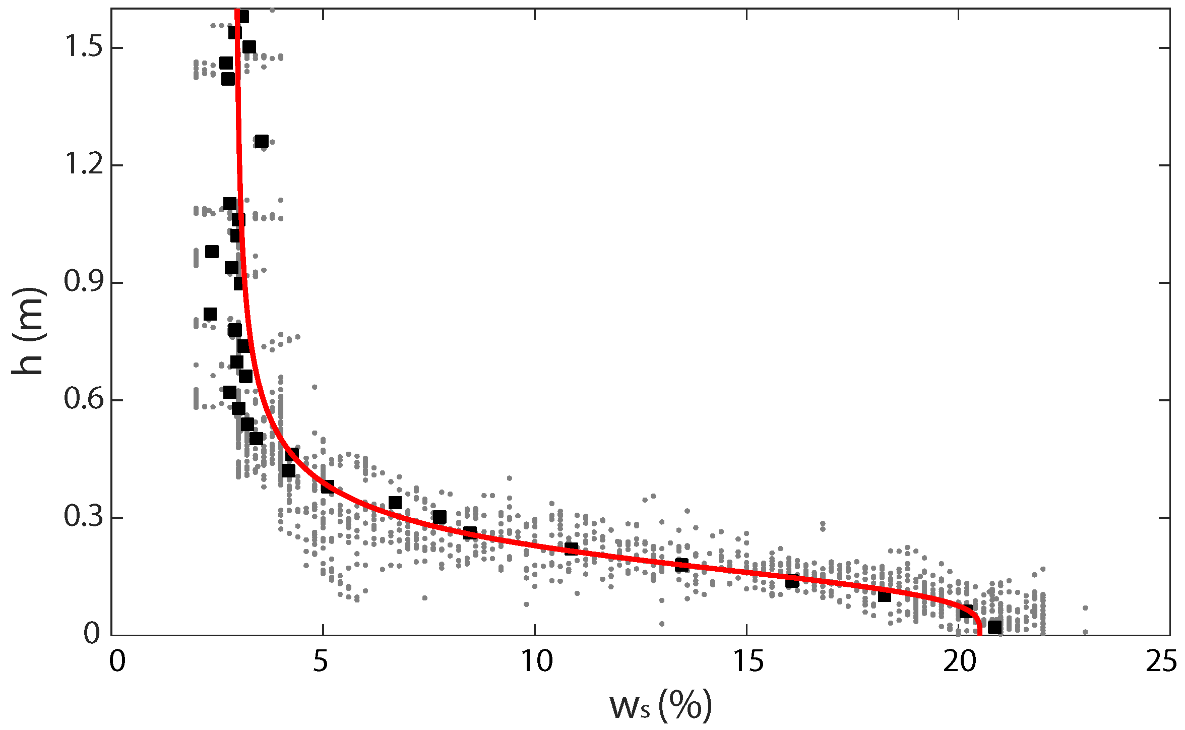
Curve fitting results in Figure 11 show a water retention curve. The data (Figure 11) show that the capillary fringe is very narrow, from the surface to approximately $h=0.05$ m. From this point, surface moisture decreases fast over a small range in groundwater depth (0.05 m–0.5 m). This indicates a homogenous soil with a narrow distribution in grain- and pore sizes and corresponds to the sieve curves and pF-curves mentioned in Section 2. Above or below this range, the curve becomes a steep almost vertical line, indicating that there is no relationship between groundwater depth and surface moisture content any more. Logically, a deeper groundwater depth leads to a lower surface moisture content.

The first cross-shore moisture zone, where the sand remains wet, always has $h<\sim$0.1 m, while the third zone, with permanently dry sand, has $h>\sim$0.4 m. In the second (intertidal) zone, h varies between 0.1–0.4 m. The steep decline in $w_s$ with h also reflects that the sand can dry rapidly with time and the sandbar can be substantially drier than its surroundings. Figure 9 illustrated that, in zone 2, the groundwater kept on falling until inundation by the rising tide. This explains why surface moisture reduced in zone 2 even during rising tide (Figure 7e,f). Finally, Figure 11 shows no evidence of hysteresis, as there is a single cloud of points, not two separate clouds that reflect a wetting and drying curve. This is not surprising as for most data points (zone 1 and 2) groundwater only falls when the beach is not submerged. In zone 3, groundwater can rise and fall, but here the tidal fluctuations are small and the groundwater sits deep (Figure 9 and Figure 10). Apparently, this does not lead to (obvious) hysteresis effects in surface moisture content.

The observed relationship between surface moisture and groundwater depth can be approximated well with the Van Genuchten (1980) equation:

$$w_s\left(h\right)=w_{res}+\frac{w_{sat}-w_{res}}{{[1+{(\alpha \mid h\mid )}^n]}^{1-\frac{1}{n}}},$$

(2)

where $w_s$ represents surface moisture content [%] and h groundwater depth [m], $w_{sat}$ saturated water content = 20.51 [L${}^3$L${}^{-3}$] and $w_{res}$ residual water content = 2.92 [L${}^3$L${}^{-3}$]. $\alpha$ = 5.59 and n = 3.69 both are fitting parameters. $\alpha$ is related to the inverse of the air entry suction and positions the curve in the vertical direction (e.g., soils with a low air entry value, like clays are positioned higher than sandy soils). n is a measure of the pore size distribution and shapes the slope of the curve (e.g., soils with a poorly sorted grain size have a steeper slope than soil that are well-sorted).

3.4. Prediction of Surface Moisture Contents with Measured Groundwater Levels

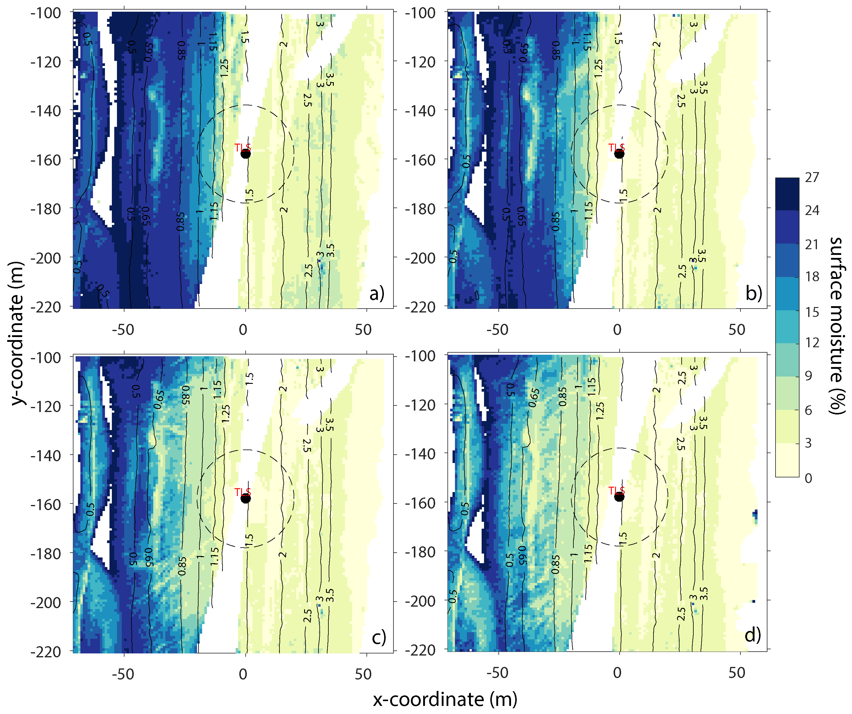
Figure 12 top row shows two TLS-derived maps, on 29 September and 29 October. Figure 12 middle row, shows corresponding calculated $1\times 1$ m low-tide surface moisture maps calculated for the same time step as the TLS-derived surface moisture maps. To create these calculated maps, groundwater height data measured with 10 pressure transducers in the cross-shore transect, were interpolated in the cross-shore direction with a spline fit and then extrapolated in the along-shore direction over a 1 × 1 m gridsize, with the assumption that groundwater levels did not vary in this direction. Subsequently, groundwater depth was calculated by subtracting the extrapolated groundwater height map from a time-corresponding TLS beach height map. By applying the obtained groundwater depth map in Equation (2), the surface moisture maps could be calculated (Figure 12 middle row).

At first glance, the calculated maps agree well with the observations. They show a similar increase in surface moisture content from land to sea, and drier sand on the bar than at its surroundings. The calculated maps, on the whole, appear to be smoother than the observations, as various small-scale variability in observed moisture content, especially just seaward of the high-tide level on 29 September is not apparent in the calculations. To better compare the maps, Figure 12 bottom row shows the alongshore median moisture content versus cross-shore distance, both for the observations (black line) and computations (blue line). For both days, we see that the measured and calculated median surface moisture content show the same zonation of surface moisture distribution with a clear division between the upper and lower part of the beach divided by the high water line, and a saturated part around the trough close to the sea. The similarity between the calculated and measured surface moisture content is largest on 29 September where both lines overlap across the entire beach. On 29 October, differences are largest in the wet zone just above the low-tide level, the calculated surface moisture content being lower than the measured value. This may have been caused by the exclusion of the effect of swash motions on moisture content close to the waterline.

4. Discussion

4.1. Relationship between Surface Moisture and Groundwater Depth

Our data illustrated that groundwater depth controls spatiotemporal surface moisture variations. As in other studies, this relationship can be described by a soil water retention curve [13,15,19,21,22,25]. However, other controlling factors such as evaporation and precipitation were not taken into account in this research. During the campaign, we did not encounter any rain showers and therefore we could not explore the influence of precipitation. To examine the influence of evaporation, we compared the Van Genuchten relationship for different days. On a day when evaporation is expected to be high, a deviation to the left in the Van Genuchten curve should be present, reflecting that, for the same groundwater depth, lower surface moisture content was measured. We noticed some difference for the dry beach in the order of 2% with lower values on the days that evaporation was expected to be highest (sunny, higher air temperature). However, we did not find a deviation in the other parts of the curve (e.g., intertidal beach or wet zone). This could mean that only the dry beach, where groundwater depth does not influence surface moisture anymore, evaporation plays a larger role.

Additionally, when taking the pF-curves of the soil into account (Figure 2), it is not surprising that evaporation does not contribute substantially to the change in surface moisture. The pF-curves show that the soil reacts as an on–off system. At a pF-value of 1.5, all the water is drained out of the soil and the horizontal line without a slope proves this happens almost at once. This means that, when groundwater depth drops below the thickness of the capillary fringe, the characteristics of the soil are causing surface moisture to drain out of the soil into the groundwater as fast as possible without the possibility for evaporation to contribute to this decrease in surface moisture. However, on the back beach, where surface moisture and groundwater are no longer related and $h>\sim$0.4 m, the soil is already dry and a small opportunity for evaporation remains to lower surface moisture by, in our case, ∼2%. Similar results were found by Schmutz and Namikas [21], in which the critical pressure head at which evaporation begins to impose a demonstrable influence on surface moisture variability was found to be $h=$ 0.9 to 1 m. Their field site has a D50 of 140 $\mathsf{\mu }$m, which is finer than Egmond beach. Therefore, the capillary fringe on their beach extends further above the phreatic groundwater level and the relationship between groundwater depth and surface moisture holds for a wider h range.

Moreover, to produce surface moisture maps from groundwater measurements, we interpolated groundwater depth between the different wells and extrapolated the cross-shore groundwater measurements in the alongshore direction, assuming alongshore uniformity in groundwater elevation. However, Figure 10 already showed that morphology seems to influence groundwater elevation locally. Because morphology varied in the along-shore direction, the assumption that groundwater elevation does not vary in the along-shore direction is most likely too simple.

Finally, to produce the Van Genuchten relationship, we used surface moisture data measured with a Theta probe instead of the TLS. The reason for this was that the TLS was purposely positioned more than 60 m from the wells to produce surface moisture maps without shading from the wells. Consequently, TLS surface moisture data next to the boreholes was deemed insufficiently accurate and was not linked to groundwater depth. In addition, the TLS was only used twice during the campaign. The 10 days of Theta probe measurements provided a substantially larger dataset to link to groundwater depth. However, Theta probe data provide surface moisture contents averaged over the top 2 cm. Hence, it would be reasonable to expect that surface moisture measured with a Theta probe is biased high with respect to the TLS values. To test this expectation, cross-shore transects of surface moisture made by the TLS were taken from the surface moisture maps within the accurate range of 60 m from the TLS. These surface moisture transects, though not directly taken next to the wells, were compared to groundwater depths measured by the pressure transducers at the same time. Although the amount of data points was substantially lower than with the Theta probe recordings, these data also show a Van Genuchten type relationship with the same capillary range and approximately the same values for the Van Genuchten parameters ($w_{res}$, $w_{sat}$, $\alpha$ and n). In addition, the median values in Figure 12 bottom row do not show a clear positive bias in the computations. On the whole, this suggests that differences between surface moisture contents and those averaged over the top 2 cm are small and that the Theta probe-based Van Genuchten relationship can be used to compute surface moisture maps.

4.2. Surface Moisture Content and Sand Transport Availability

Consistent with the recent studies of Brakenhoff et al. [22] and Schmutz and Namikas [21], our research confirms that the beach can be conceptualized into three surface moisture zones; the wet zone ($w_s>25\%$), intertidal zone ($w_s\sim$ 5–25%) and the dry zone ($w_s<5\%$). The presence of a bar–trough system acts as a perturbation to this overall cross-shore zonation and these should be characterized as separate morphological features. The trough belongs to the wet zone, since it never dries out and is either completely saturated or inundated by the sea. The sandbar shows characteristics of the upper intertidal zone, and can reach surface moisture values below 10%. Delgado-Fernandez [10] states that, depending on wind characteristics, sand with a surface moisture content below 10% has a chance to be picked up by the wind. Surface moisture content above 10% prohibits sand transport entirely, while sand with surface moisture content below 4% is always available for aeolian sand transport. Our surface moisture maps can be used for which part of the beach is potentially available for aeolian transport. During our field campaign, we observed that sand at the back beach, if not inundated due to a storm event, was always available for aeolian sand transport. In the wet zone, sand is most likely never available for aeolian sand transport and in the intertidal zone sand becomes available for aeolian sand transport, since surface moisture can decrease from complete saturation 25% to below 10% within a single ebb tidal cycle. Whether dry sand on the sandbar is available for aeolian transport and capable of saltating across the wet trough is not clear. From moisture observations on a multi-barred beach, Anthony et al. [16] inferred that the troughs prohibit sand on the bars to be blown toward the dry beach and that only sand on the dry beach can reach the foredunes. However, during our fieldwork campaign, sand transport from the sandbar crossing the trough and reaching the dune foot was sometimes observed. Further research is needed to determine the trough characteristics (e.g., width) that fully or only partly block onshore aeolian transport.

The next step in our research will be to model spatiotemporal groundwater elevation (2D) with ModFlow [41,42]. In this way, we hope to gain more insight in alongshore varying groundwater fluctuations and to improve the accuracy of the predicted surface moisture maps. Additionally, we want to investigate what the influence of a bar–trough system will be on sand transport availability. Finally, we wish to couple the tidal–groundwater–surface moisture model to an aeolian fetch model of, for example, Bauer and Davidson-Arnott [3] or the advection model of De Vries et al. [43] to produce better estimations of aeolian sand transport from the beach into the dune than possible with wind-only models.

5. Conclusions

With our TLS-derived, high-resolution, spatiotemporal surface moisture maps, we have shown how surface moisture varies during falling and rising tide on a mildly sloping (∼1:30) beach consisting predominantly of quartz sand with a well sorted grain size distribution (D50 = 250–300 $\mathsf{\mu }$m). The beach can be conceptualized into three surface moisture zones, namely: the wet zone (∼18–25%), the intertidal zone (∼5–25%) and the back beach (∼$3\%$). Over time, the intertidal zone shows the largest fluctuations, whereas the back beach and the wet zone stay rather dry and saturated, respectively. The bar–trough system perturbs this overall pattern with the bar showing moisture characteristics as the upper intertidal beach and the trough as the wet zone. During falling tide, the beach and especially the sandbar dries out until it inundates by the rising tide. No anticipated processes by capillary forces in front of the rising tide are present. A Van Genuchten curve describes the relationship between surface moisture and groundwater depth well, with no indication of hysteresis effects. With this Van Genuchten curve, surface moisture maps can be calculated from groundwater depth measurements; however, our assumption of alongshore uniformity in groundwater elevation may be too simple. Other factors, like evaporation, appear to be less important to surface moisture dynamics.

References

- van Gent, M.R.A.; de Vries, J.V.T.; Coeveld, E.M.; De Vroeg, J.H.; Van de Graaff, J. Large-scale dune erosion tests to study the influence of wave periods. Coast. Eng. 2008, 55, 1041–1051. [Google Scholar] [CrossRef]
- Roelvink, D.; Reniers, A.; van Dongeren, A.; van Thiel de Vries, J.; McCall, R.; Lescinski, J. Modelling storm impacts on beaches, dunes and barrier islands. Coast. Eng. 2009, 56, 1133–1152. [Google Scholar] [CrossRef]
- Bauer, B.O.; Davidson-Arnott, R.G.D. A general framework for modeling sediment supply to coastal dunes including wind angle, beach geometry, and fetch effects. Geomorphology 2002, 49, 89–108. [Google Scholar] [CrossRef]
- Delgado-Fernandez, I. A review of the application of the fetch effect to modelling sand supply to coastal foredunes. Aeolian Res. 2010, 2, 61–70. [Google Scholar] [CrossRef] [Green Version]
- Keijsers, J.G.S.; de Groot, A.V.; Riksen, M.J.P.M. Modeling the biogeomorphic evolution of coastal dunes in response to climate change. J. Geophys. Res. Earth Surf. 2016, 121, 1161–1181. [Google Scholar] [CrossRef]
- Hoonhout, B.M.; De Vries, S. A process-based model for aeolian sediment transport and spatiotemporal varying sediment availability. J. Geophys. Res. Earth Surf. 2016, 121, 1555–1575. [Google Scholar] [CrossRef] [Green Version]
- Sarre, R.D. Evaluation of aeolian sand transport equations using intertidal zone measurements, Saunton Sands, England. Sedimentology 1988, 35, 671–679. [Google Scholar] [CrossRef]
- Davidson-Arnott, R.G.D.; Law, M.N. Measurements and prediction of longterm sediment supply to coastal foredunes. J. Coast. Res. 1996, 12, 654–663. [Google Scholar]
- Keijsers, J.G.S.; Poortinga, A.; Riksen, M.J.P.M.; Maroulis, J. Spatio-temporal variability in accretion and erosion of coastal foredunes in the netherlands: Regional climate and local topography. PLoS ONE 2014, 9, e91115. [Google Scholar] [CrossRef]
- Delgado-Fernandez, I. Meso-scale modelling of aeolian sediment input to coastal dunes. Geomorphology 2011, 130, 230–243. [Google Scholar] [CrossRef] [Green Version]
- Namikas, S.; Sherman, D. Desert Aeolian Processes; Chapter A Review of the Effects of Surface Moisture Content on Aeolian Sand Transport; Springer: Dordrecht, The Netherlands, 1995; pp. 269–293. [Google Scholar]
- Darke, I.; Davidson-Arnott, R.; Ollerhead, J. Measurement of Beach Surface Moisture Using Surface Brightness. J. Coast. Res. 2009, 251, 248–256. [Google Scholar] [CrossRef]
- McKenna Neuman, C.; Langston, G. Measurement of water content as a control of particle entrainment by wind. Earth Surf. Process. Landf. 2006, 31, 303–317. [Google Scholar] [CrossRef]
- Schmutz, P.P.; Namikas, S.L. Utility of the Delta-T Theta Probe for Obtaining Surface Moisture Measurements from Beaches. J. Coast. Res. 2011, 27, 478–484. [Google Scholar] [CrossRef]
- Namikas, S.L.; Edwards, B.L.; Bitton, M.C.A.; Booth, J.L.; Zhu, Y. Temporal and spatial variabilities in the surface moisture content of a fine-grained beach. Geomorphology 2010, 114, 303–310. [Google Scholar] [CrossRef]
- Anthony, E.J.; Ruz, M.; Vanhee, S. Aeolian sand transport over complex intertidal bar–trough beach topography. Geomorphology 2009, 105, 95–105. [Google Scholar] [CrossRef]
- Nield, J.M.; King, J.; Jacobs, B. Detecting surface moisture in aeolian environments using terrestrial laser scanning. Aeolian Res. 2014, 12, 9–17. [Google Scholar] [CrossRef]
- Smit, Y.; Ruessink, B.G.; Brakenhoff, L.B.; Donker, J.J.A. Measuring the spatial and temporal variation in surface moisture on a coastal beach with an infra-red terrestrial laser scanner. Aeolian Res. 2018, 31, 19–27. [Google Scholar] [CrossRef]
- Yang, Y.; Davidson-Arnott, R.G.D. Rapid measurement of surface moisture content on a beach. J. Coast. Res. 2005, 21, 447–452. [Google Scholar] [CrossRef]
- Bauer, B.O.; Davidson-Arnott, R.; Hesp, P.; Namikas, S.; Ollerhead, J.; Walker, I. Aeolian sediment transport on a beach: Surface moisture, wind fetch, and mean transport. Geomorphology 2009, 105, 106–116. [Google Scholar] [CrossRef]
- Schmutz, P.P.; Namikas, S.L. Measurement and modeling of the spatiotemporal dynamics of beach surface moisture content. Aeolian Res. 2018, 34, 35–48. [Google Scholar] [CrossRef]
- Brakenhoff, L.; Smit, Y.; Donker, J.; Ruessink, G. Tide-induced variability in beach surface moisture: Observations and modelling. Earth Surf. Process. Landf. 2018, 1, 1–5. [Google Scholar] [CrossRef]
- Oblinger, A.; Anthony, E.J. Surface Moisture Variations on a Multibarred Macrotidal Beach: Implications for Aeolian Sand Transport. J. Coast. Res. 2008, 24, 1194–1199. [Google Scholar] [CrossRef]
- Atherton, R.J.; Baird, A.J.; Wiggs, G.F.S. Inter-tidal Dynamics of Surface Moisture Content on a Meso-tidal Beach. J. Coast. Res. 2001, 17, 482–489. [Google Scholar]
- Darke, I.; McKenna Neuman, C. Field Study of Beach Water Content as a Guide to Wind Erosion Potential. J. Coast. Res. 2008, 245, 1200–1208. [Google Scholar] [CrossRef]
- Schmutz, P.P.; Namikas, S.L. Measurement and modeling of moisture content above an oscillating water table: Implications for beach surface moisture dynamics. Earth Surf. Process. Landf. 2013, 38, 1317–1325. [Google Scholar] [CrossRef]
- Ruz, M.H.; Meur-Ferec, C. Influence of high water levels on aeolian sand transport: Upper beach/dune evolution on a macrotidal coast, Wissant Bay, northern France. Geomorphology 2004, 60, 73–87. [Google Scholar] [CrossRef]
- Chuang, M.H.; Yeh, H.D. An analytical solution for the head distribution in a tidal leaky confined aquifer extending an infinite distance under the sea. Adv. Water Resour. 2006, 30, 439–445. [Google Scholar] [CrossRef]
- Van Genuchten, M.T. A closed-form equation for predicting the hydraulic conductivity of unsaturated soils. Soil Sci. Soc. Am. J. 1980, 44, 892–898. [Google Scholar] [CrossRef]
- Childs, E.C.; Poulovassilis, A. The moving profile above a moving water table. J. Soil Sci. 1962, 13, 272–285. [Google Scholar] [CrossRef]
- Gallage, C.P.K.; Uchimura, T. Effects of dry density and grain size distribution on soil-water characteric curves of sandy soil. Soils Found. 2010, 50, 161–172. [Google Scholar] [CrossRef]
- Pape, L.; Plant, N.; Ruessink, B. On cross-shore migration and equilibrium states of nearshore sandbars. J. Geophys. Res. 2010, 115. [Google Scholar] [CrossRef] [Green Version]
- Masselink, G.; Kroon, A.; Davidson-Arnott, R.G.D. Morphodynamics of intertidal bars in wave-dominated coastal settings—A review. Geomorphology 2006, 73, 33–49. [Google Scholar] [CrossRef]
- De Winter, R.C.; Gongriep, F.; Ruessink, B.G. Observations and modeling of alongshore variability in dune erosion at Egmond aan Zee, the Netherlands. Coast. Eng. 2015, 99, 167–175. [Google Scholar] [CrossRef]
- Van Enckevort, I.M.J.; Ruessink, B.G. Effect of hydrodynamics and bathymetry on video estimates of nearshore sandbar position. J. Geophys. Res. 2001, 106, 16969–16979. [Google Scholar] [CrossRef] [Green Version]
- Dane, J.; Hopmans, J. Methods of Soil Analysis: Part 4. Physical Methods; Soil Science Society of America Book Series; Soil Science Society of America: Washington, DC, USA, 2002; Volume 5. [Google Scholar]
- Plant, N.G.; Holland, K.T.; Puleo, J.A. Analysis of the scale of errors in 696 nearshore bathymetric data. Mar. Geol. 2002, 191, 71–86. [Google Scholar] [CrossRef]
- Tsegaye, T.D.; Tadesse, W.; Coleman, T.L.; Jackson, T.J.; Tewolde, H. Calibration and modification of impedance probe for near surface soil moisture measurements. Can. J. Soil Sci. 2004, 84, 237–243. [Google Scholar] [CrossRef] [Green Version]
- Nielsen, P. Tidal Dynamics of the Water Table in Beaches. Water Resour. Res. 1990, 26, 2127–2134. [Google Scholar] [CrossRef]
- Raubenheimer, B.; Guza, R.T.; Elgar, S. Tidal water table fluctuations in a sandy ocean beach. Water Resour. Res. 1999, 35, 2313–2320. [Google Scholar] [CrossRef] [Green Version]
- Schmitz, O.; Karssenberg, D.; van Deursen, W.P.; Wesseling, C.G. Linking external components to a spatio-temporal modelling framework: Coupling MODFLOW and PCRaster. Environ. Model. Softw. 2009, 24, 1088–1099. [Google Scholar] [CrossRef]
- Pauw, P.S.; Oude Essink, G.H.P.; Leijnse, A.; Vandenbohede, A.; Groen, J.; van der Zee, S.E.A.T.M. Regional scale impact of tidal forcing on groundwater flow in unconfined coastal aquifers. J. Hydrol. 2014, 517, 269–283. [Google Scholar] [CrossRef]
- De Vries, S.; Van Thiel de Vries, J.; Van Rijn, L.C.; Arens, S.; Ranasinghe, R. Aeolian sediment transport in supply limited situations. Aeolian Res. 2014, 12, 75–85. [Google Scholar] [CrossRef]
Figure 1.
The study site is located south of Egmond aan Zee, between beach poles 41 and 42. The photograph on the right was taken from the Argus tower [35] and illustrates that the beach is fairly narrow and backed by a high foredune.
Figure 2.
pF curves of the soil at Egmond Beach, made with nine samples. All samples with number 1 were taken at the same location in the swash zone, samples with number 2 were taken at the same location on the intertidal beach and samples with the number 3 were taken at the same location near the dune foot. The letters a, b and c mean ∼0–6 cm, ∼10–16 cm and ∼20–26 cm depth, respectively.
Figure 3.
Example of a surface moisture map made with the Terrestrial Laser Scanner (TLS) on 29 September 2015 with a grid size of 1 × 1 m. The darker blue colors represent high surface moisture content with a maximum of 25% and lighter yellow colors represent low surface moisture content with a minimum of 3%. Positive x is landward, and positive y is to the north. W1–W10 indicate the position of the groundwater wells in a cross-shore array and the circle around the TLS indicates values that are less reliable according to Smit et al. [18]. The contours are elevation with respect to Mean Sea Level.
Figure 4.
Side view of beach height profiles, taken on the same 10 days of Theta probe measurements, with the groundwater wells indicated by W1–W10. Note how the sandbars move over time from the sea towards the dunes (a–c).
Figure 5.
Time series of offshore (a) water level, (b) significant wave height and (c) wind speed from 21 September until 2 November 2015 measured at IJmuiden (approximately 15 km to the south of Egmond). The red line represents conditions during Theta probe measurements and the blue line during TLS measurements.
Figure 6.
Four surface moisture maps taken over time on 29 September 2015 during falling tide. (a) 10:32 a.m.; (b) 12:30 p.m.; (c) 2:00 p.m. and (d) 3:45 p.m. Note that the TLS in the middle of the maps, the sandbar on the left with lighter colours and the trough right next to it with no datapoints because it is inundated.
Figure 7.
Surface moisture dynamics and beach morphology during falling and rising tide on 29 September and 29 October 2015. (a,b) show the median of all beach height (z) values of the same x-coordinate for 29 September and 29 October, respectively, in a side view from the sea (left) towards the dunes (right); (c,d) show the median of all surface moisture measurements along the same x-coordinate for the indicated time step when a TLS survey was conducted (per half an hour) during falling tide; (e,f) show the same information as the (c,d) only during rising tide and the time interval between the TLS surveys is set to 15 min. Note the high water line on 29 September lies around m and for 29 October around m.
Figure 8.
All surface moisture values (gray dots) from all the TLS surveys per day, plotted against their x-coordinate. (a) contains 19 surveys measured on 29 September; (b) contains 22 surveys measured on 29 October. For both panels, the median (black line) and 2.5 and 97.5 percentile (blue lines) are plotted.
Figure 9.
Time series of elevations on (a) 29 September 2015 and (b) on 29 October 2015. The different line colors represent different pressure transducers W1 (sea) to W10 (dune foot). On 29 September, the pressure transducer in the sea which measures tidal fluctuations was working properly and is represented by the black line.
Figure 10.
Groundwater levels over a cross-shore transect during falling tide on (a) 29 September and (b) 29 October 2015. The different colors show different moments in time. At each time step a corresponding surface moisture map by the TLS was taken.
Figure 11.
Groundwater depth (h) versus surface moisture content (). The gray dots are the individual observations measured with the Theta probe. The squares are the mean values in 0.04 m bins. The red line is the fitted Van Genuchten relationship, (Equation (2)), to the binned values. The is 0.997 and the standard error is 0.44%.
Figure 12.
Measured (top row) versus calculated (middle row) surface moisture maps, presented in a 1 × 1 m grid, taken on 29 September 2015. The bottom row shows the median of all surface moisture measurements along the same x-coordinate for 18 measured surface moisture maps (black line) and 18 calculated surface moisture maps (blue line), for the same time steps as the measured surface moisture maps. Note: both lines show the same pattern and beach zones.
© 2019 by the authors. Licensee MDPI, Basel, Switzerland. This article is an open access article distributed under the terms and conditions of the Creative Commons Attribution (CC BY) license (http://creativecommons.org/licenses/by/4.0/).
Share and Cite
MDPI and ACS Style
Smit, Y.; Donker, J.J.A.; Ruessink, G. Spatiotemporal Surface Moisture Variations on a Barred Beach and their Relationship with Groundwater Fluctuations. Hydrology 2019, 6, 8. https://doi.org/10.3390/hydrology6010008
AMA Style
Smit Y, Donker JJA, Ruessink G. Spatiotemporal Surface Moisture Variations on a Barred Beach and their Relationship with Groundwater Fluctuations. Hydrology. 2019; 6(1):8. https://doi.org/10.3390/hydrology6010008
Chicago/Turabian StyleSmit, Yvonne, Jasper J. A. Donker, and Gerben Ruessink. 2019. "Spatiotemporal Surface Moisture Variations on a Barred Beach and their Relationship with Groundwater Fluctuations" Hydrology 6, no. 1: 8. https://doi.org/10.3390/hydrology6010008
Note that from the first issue of 2016, this journal uses article numbers instead of page numbers. See further details here.