On the Relationship between Experimental and Numerical Modelling of Gravel-Bed Channel Aggradation


Department of Civil and Environmental Engineering, Politecnico di Milano, 20133 Milan, Italy
*
Author to whom correspondence should be addressed.
Hydrology 2019, 6(1), 9; https://doi.org/10.3390/hydrology6010009
Submission received: 23 December 2018
/
Revised: 11 January 2019
/
Accepted: 13 January 2019
/
Published: 15 January 2019
(This article belongs to the Special Issue Catchments Hydrology and Sediment Dynamics: Concepts, Measuring and Modelling)
Abstract
:This communication explores the use of numerical modelling to simulate the hydro-morphologic response of a laboratory flume subject to sediment overloading. The numerical model calibration was performed by introducing a multiplicative factor in the Meyer–Peter and Müller transport formula, in order to achieve a correspondence with the bed and water profiles recorded during a test carried out under a subcritical flow regime. The model was validated using a second subcritical test, and then run to simulate an experiment during which morphological changes made the water regime switch from subcritical to supercritical. The “relationship” between physical and numerical modelling was explored in terms of how the boundary conditions for the two approaches had to be set. Results showed that, even though the first two experiments were reproduced well, the third one could not be modeled adequately. This was explained considering that, after the switch of the flow regime, some of the boundary conditions posed into the numerical model turned out to be misplaced, while others were lacking. The numerical modelling of hydro-morphologic processes where the flow regime is trans-critical in time requires particular care in the position of the boundary conditions, accounting for the instant at which the water regime changes.
1. Introduction
River morphologic processes are among the most important agents that shape the Earth’s surface. These phenomena have been extensively studied for decades due to a major relevance for a number of applications, such as watercourse management, design of hydraulic structures, land use planning, flood risk evaluation, water quality, and habitat creation (e.g., [1,2,3,4,5,6,7,8,9,10]). Stemming from ongoing research projects by the authors, this communication considers specifically the aggradation processes resulting from sediment overloading of an open channel, with a focus on situations relevant for mountainous environments.
Mathematical modelling, coupled with numerical simulation, is widely used for the computation of bed and water levels in alluvial streams or channels. Two different approaches may be taken when choosing a domain of interest to be modelled: in a first approach, a whole catchment may be considered (e.g., [11,12,13]); otherwise, a model may include a particular river reach at stake, with the resulting need to appropriately quantify the water and sediment fluxes at the boundaries (see, for example, [3,5,6,14]), sometimes with simplifying assumptions of equilibrium transport conditions (e.g., [4,8,15]). Within the second approach, applications of numerical modelling to mountain environments are mostly based on the one-dimensional shallow water equations (e.g., [16,17,18]), because lateral diversions of water with respect to the main flow direction are limited. Numerical models need to be calibrated based on field or laboratory data. Since field observations of degradation/aggradation dynamics are often very challenging due to complex natural conditions and a great amount of human effort required, laboratory experiments have been traditionally used to mimic the hydro-morphologic processes that occur in reality and to calibrate numerical simulations (frequently leading to companion papers, e.g., [19,20]). Furthermore, laboratory tests enable a deep insight to be obtained of the mechanisms governing the observed phenomena, since laboratory conditions are obviously better controlled than the field ones. In the context of aggradation processes due to channel overloading, numerous experimental investigations have been conducted in the past covering a wide range of flow and sediment loading conditions (see, for example, [21,22,23,24,25,26,27,28,29]), with the aim of improving the phenomenological characterization of the process.
The objective of this contribution is to further discuss the “relationship” between experimental and numerical modelling of bed aggradation due to overloading in an open channel; specifically, the study explores how the boundary conditions for the two approaches have to be set and how they act. Hydro-morphologic experiments were carried out in a straight channel. The laboratory flume was overloaded by an upstream sediment feeding that mimicked a sediment load from an upstream part of a catchment, shallow landslide or tributary reach. To characterize the hydro-morphologic response of the channel, several quantities of interest were simultaneously measured at adequate spatial and temporal resolutions. Corresponding one-dimensional numerical simulations were performed, imposing initial and boundary conditions equal to the controls that were used in the laboratory runs. The numerical model was calibrated with reference to a single test, then applied to the other tests for validation. Different levels of agreement were detected depending on the flow regime (stably subcritical or transient to supercritical). We investigate how accurately the morphologic evolution is reproduced by the numerical model under different conditions; moreover, a key feature of this work is the emphasis given to the “relationship” between the experimental and numerical boundary conditions. The present manuscript is structured as follows: Section 2 describes the laboratory facility and the numerical model that was used; results are presented in Section 3 and then discussed in Section 4.
2. Experimental and Numerical Modelling
2.1. Laboratory Facility and Experimental Tests
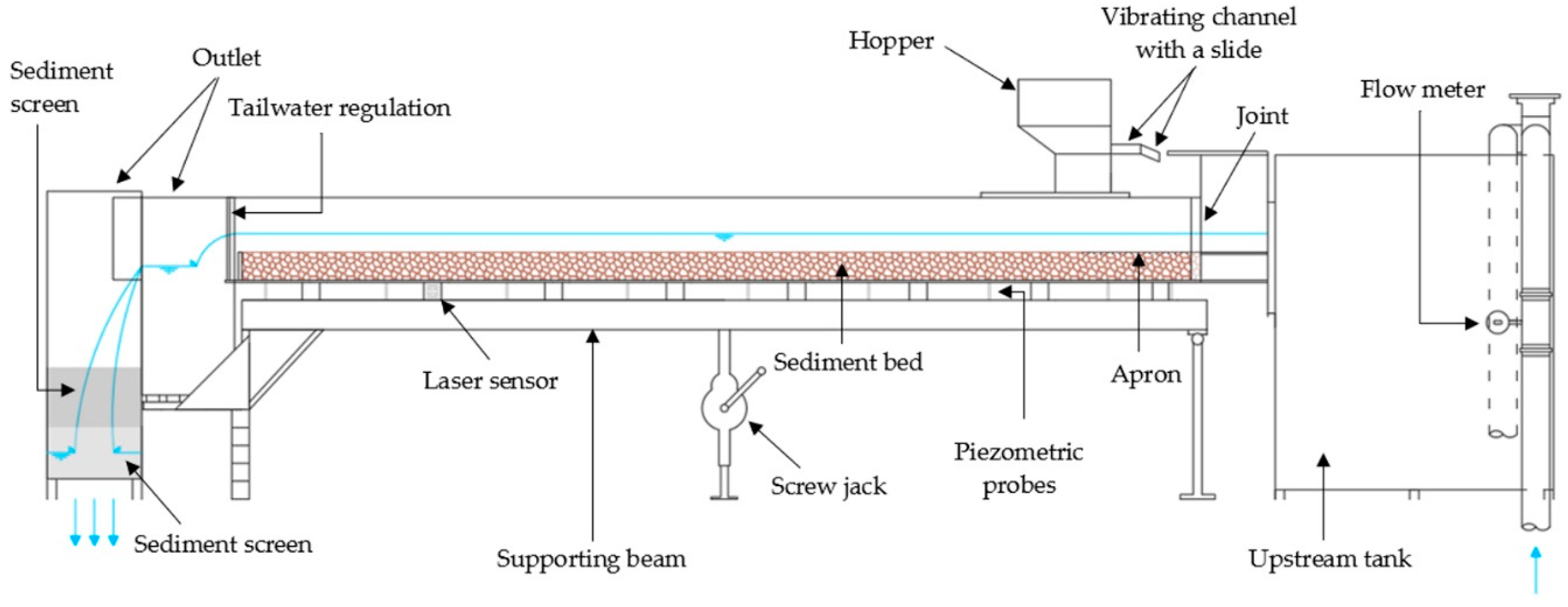
The aggradation experiments were performed at the Mountain Hydraulics Laboratory of the Politecnico di Milano using a tilting flume (5.2 m long, 0.3 m wide, and 0.45 m deep) with a rectangular cross-section (Figure 1) and a slope set at 0.004. The channel was filled with a 15 cm layer of polyvinyl chloride (PVC) cylindrical particles (mean diameter d = 3.8 mm, geometric standard deviation of the grain size distribution σg = 1.04, density ρs = 1443 kg/m3, and porosity p = 0.45), bounded downstream by a sill. Inlet scour is prevented by a 0.75 m long apron. A tail-water regulation was used to impose the water level at the downstream end of the flume, and nine piezometers were present to monitor the profile of the free surface. At the inlet section, sediment may be fed by a 0.16 m wide vibrating channel equipped with a hopper. More details about the experimental facility are given by References [26,27,29].
The experiments were carried out with different hydrodynamic and overloading conditions (numerical details for the test cases presented are reported in Table 1). Each run was characterized by a water discharge Q, a sediment feeding rate QBin, and a water depth at the downstream control section hd. Experiments were designed ensuring that Q was higher than the threshold discharge Qc for sediment transport, and QBin exceeded the transport capacity of the flow QB0. Furthermore, hd was set equal to or higher than the uniform flow value h0 for the initial slope of 0.004. The quantities Qc and QB0 were known from preliminary tests (reported by References [27,29]). Before starting an aggradation experiment, the flume was filled at a very low discharge in order to avoid sediment transport. To start the aggradation phase, the flow rate was increased to the target value, the prescribed water depth was imposed at the channel outlet with the tail-water regulation, and the sediment feeder was switched on. During each run, the water and solid discharges were maintained constant; furthermore, the tail-water regulation was rearranged if needed to maintain the downstream depth constant. The sediment feeding rate, the profiles of the free surface, the profile of the flume bed, and the sediment discharge at the flume outlet were measured from movies of different parts of the experimental facility, taken during the experiments with action cameras. A detailed description of the image processing algorithms was provided by References [27,29,30].
The aggradation tests (T1, T2, and T3) presented in this manuscript are part of an extensive experimental campaign carried out over the last two years ([26,27,28,29]; specifically, T1, T2, and T3 are runs AE11, AE21, and AE17 in Reference [29]). Table 1 furnishes the main parameters of each test, including T = duration of the experiment, Ud = mean velocity at the downstream control section, and Frd = Froude number at the downstream control section.
2.2. Morphological Numerical Tool and Modelling Strategy
River morphologic processes may be represented by means of the one-dimensional Saint-Venant–Exner partial differential equations [31]. Considering a uniform bed material, negligible suspended sediment transport and the absence of lateral water and solid inflows, the system assumes the following form:
where: A = wetted cross-section area, β = momentum coefficient, g = gravity acceleration, zB = bed elevation, h = water depth, Sf = friction slope, qB = bed-load flux per unit width, slB = source term specifying a local input or output of material (per unit width), t = time, and x = stream-wise coordinate. The first two equations express the conservation of mass and momentum for the liquid phase, while the third one imposes the continuity for the solid fraction. Two closure equations are needed to mathematically close the system. The first equation expresses the friction slope Sf as:
where: cf = dimensionless friction coefficient, n = Manning roughness coefficient, and R = hydraulic radius. The determination of cf is based on the approach by Strickler [32]:
The second closure equation is the sediment transport formula by Meyer–Peter and Müller [33] (abbreviated to “MPM” henceforth), which quantifies the bed-load transport rate as:
where: s = ρs/ρ, with ρ as the water density, θ = Shields [34] parameter, and the subscript c indicates the threshold conditions. According to van Rijn [35], θc may be evaluated as a function of the dimensionless grain diameter D*:
where D* is defined as (ν = kinematic viscosity of water):
Obviously, initial and boundary conditions are needed to solve the system. Initial conditions must be specified for the water depth h, liquid discharge Q, and bed elevation zB in the whole computational domain. Boundary conditions for the independent variables h, Q, and zB have also to be appropriately provided.
In the present study, the numerical simulation of the aggradation tests were performed using the software Basement v.2.8.0 (Basic Simulation Environment for Computation of Environmental Flow and Natural Hazard Simulations), provided by the ETH Zürich (Switzerland), e.g., [36]. The time discretization of the system (1) was based on the explicit Euler scheme, whereas the finite volume method was used in space. Among different solution schemes, the Roe [37] was chosen. The geometric model of the experimental flume included 101 rectangular cross-sections with a spacing of 4.9 cm. The computational domain was thus 4.9 m long and the channel slope was set as equal to that of the experimental flume. The length of the numerical model was slightly lower than the length of the flume (5.2 m) because the upstream section corresponded to the sediment injection point, located 25 cm downstream of the flume inlet, while the last section corresponded to the sill at the flume outlet. The sediment size, porosity, and density were the same as the experimental ones. The roughness coefficient n was set equal to the value (0.015 s/m1/3) determined experimentally by Reference [26]. A critical Shields parameter θc = 0.048 was derived by applying (5) and (6). Finally, the original MPM Formula (4) was modified, introducing two calibration parameters α and m, as follows:
Initial conditions were obtained as outputs of preliminary simulations in clear water, at the end of which a steady state was reached. Constant values for the water discharge Q and the water depth h were specified at the channel inlet and at the downstream section of the computational domain, respectively. The upstream boundary condition for zB was numerically translated into one for the sediment feeding rate per unit width qBin through Equation (8), derived by applying the backward finite difference approximation to the spatial terms of the sediment continuity equation:
where z is the bed level, and ∆t and ∆x the temporal and spatial discretization intervals; the subscript 1 indicates the upstream node of the computational domain, whereas the superscripts k and k + 1 represent two consecutive time instants. Furthermore, even though three boundary conditions are theoretically needed to close the system (1), the software Basement requires an additional condition at the downstream end, where all the sediment entering the last computational cross-section must leave the downstream boundary (i.e., the downstream bed level is fixed). This condition was necessary because, by default, the software does not consider any sediment flow across the downstream boundary. In this way, an inconsistency is created between the numerical model and the theoretical formulation. However, the numerical model is instead similar to the experimental setup where a sill is present at the channel outlet.
3. Results
3.1. Phenomenological Description of the Experimental Aggradation Profiles
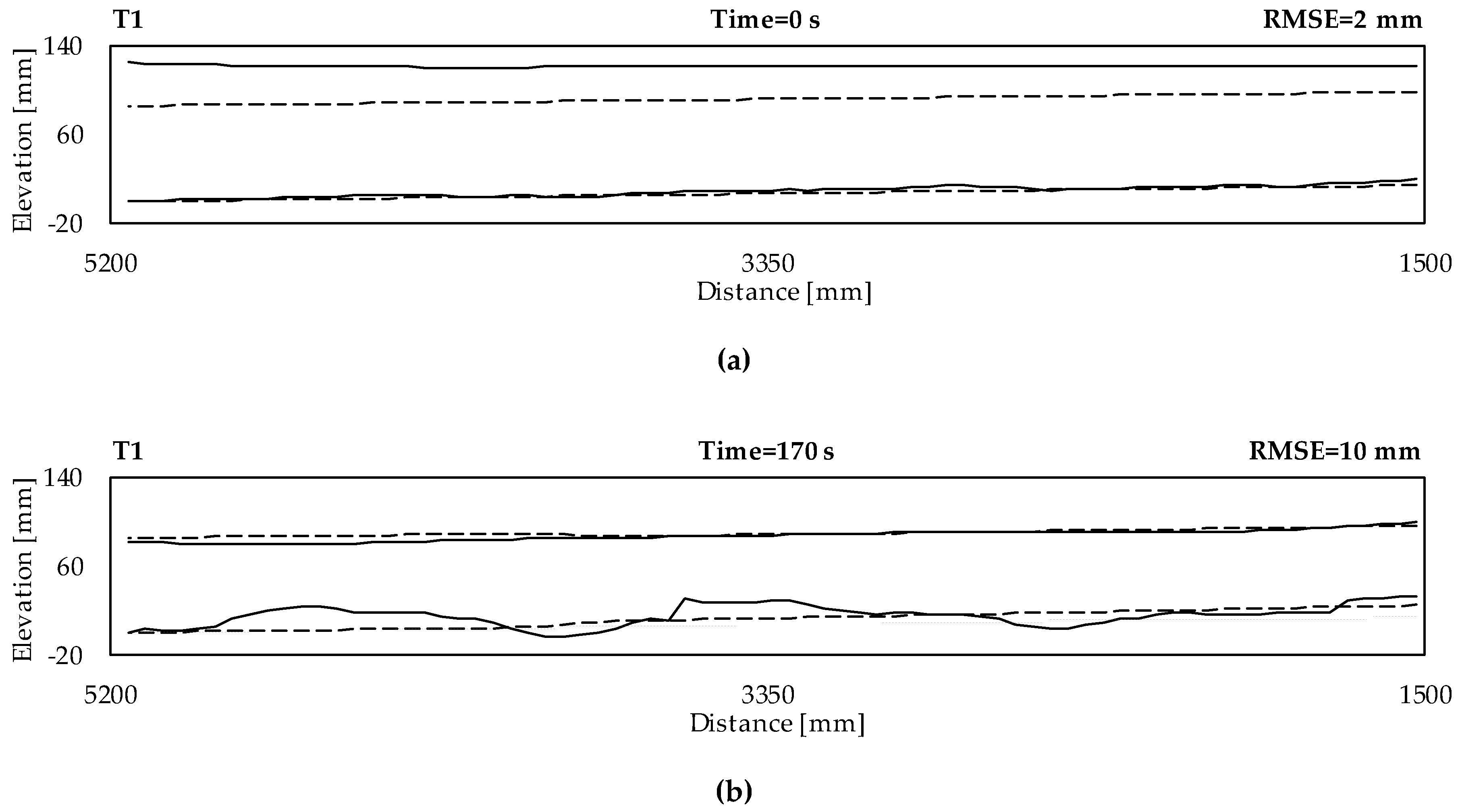
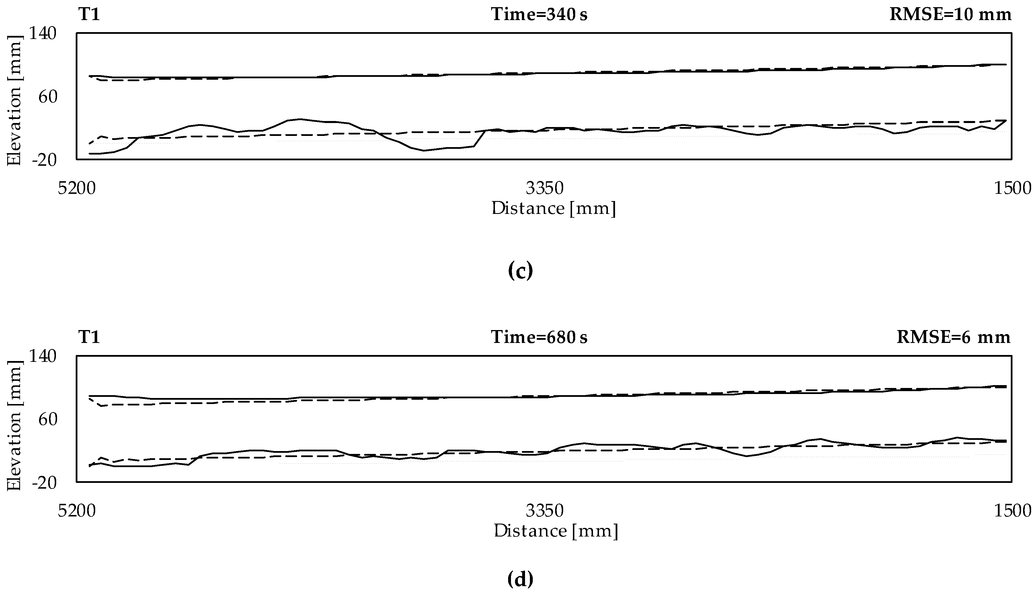
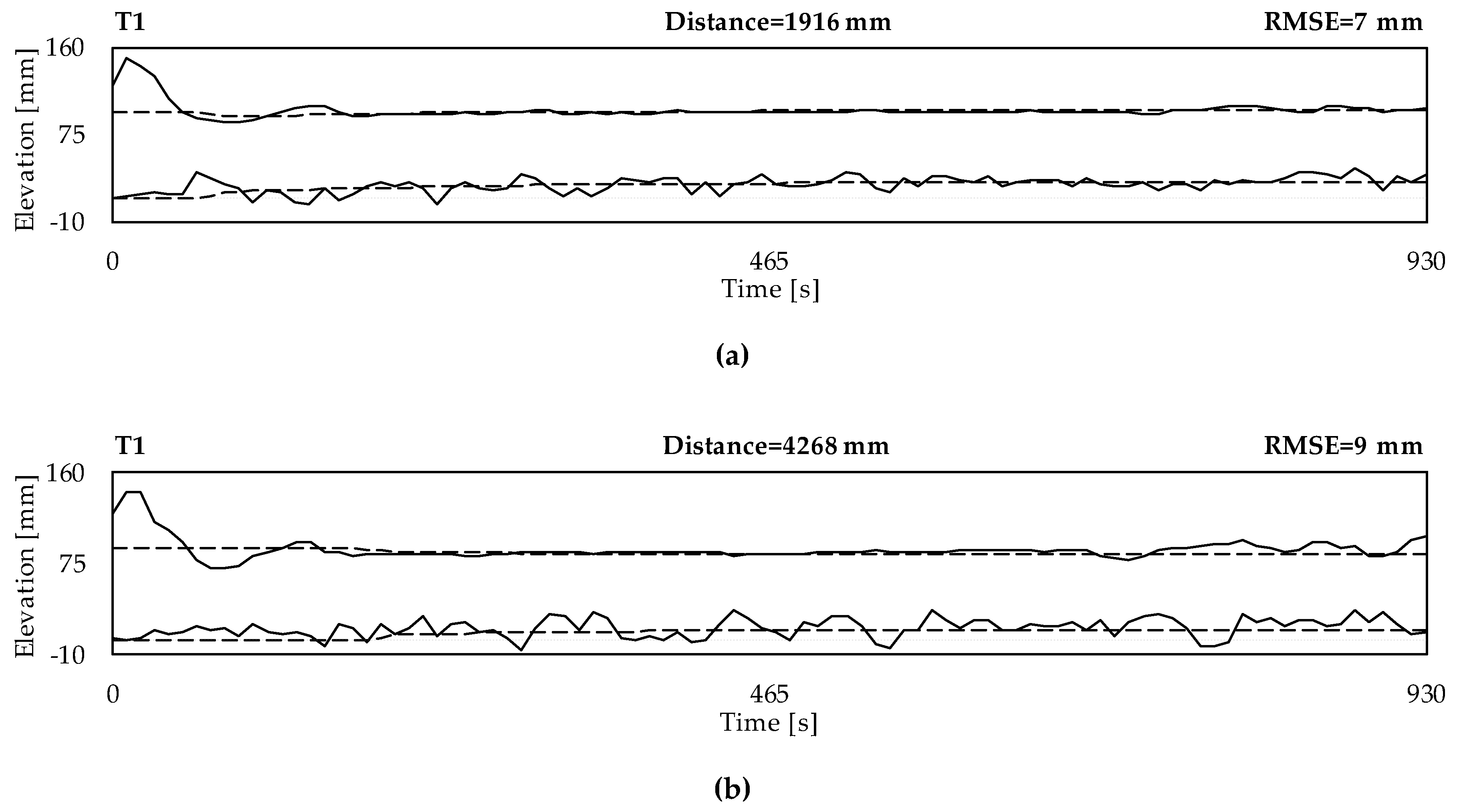
Figure 2 and Figure 3 show the spatial and temporal evolutions, respectively, of the water and bed levels (continuous black lines) for test T1 of Table 1. The measured profiles depict some key features of the process of aggradation. The deposition of particles started at the feeding section, leading to an obvious increase of the average bed elevation and the development of an aggrading sediment front. As the experiment proceeded, the reach where bed aggradation occurred lengthened progressively. Superimposed bedforms were visible as oscillations of the bed surface, both upstream and downstream of the aggradation front. As most of these structures were asymmetrical with a steep downstream slope, dunes seemed to be the dominant bedforms. Local erosion due to the troughs between following dunes was also observed. Analogous morphological characteristics were found in all the flume aggradation experiments of References [26,27,28,29], in agreement with prior literature descriptions (particularly those of References [24]). One interesting remark is that the fixed bed elevation at the downstream sill was not always respected. Furthermore, the water surface had the highest fluctuations recorded at the beginning and end of each experiment as a result of tail-water regulations. The spatial profiles depicted a tendency to oscillations of the free surface in phase opposition to the bed changes, as expected in a subcritical flow.
The observed morphological features were reasonably interpreted as follows. Since the sediment feeding rate was larger than the transport capacity of the flow, sediment deposited downstream of the feeding section. The continuous sediment supply forced the deposition front to migrate downstream. At the same time, the slope of the bed progressively increased to make the system attain a transport capacity in equilibrium with the feeding rate. The subcritical water profile obviously reacted to the modified bed morphology, assuming lower elevations above the deposition reach. An important, consequent dynamics resulted from the choice of imposing a constant water depth at the downstream end of the flume. Since the propagation of the aggradation front determined an increase of the mean longitudinal bed slope, the water depth imposed at the flume outlet always determined a backwater in the downstream portion of the flume. The reduced sediment transport capacity of the backwatered profile generally caused sediment deposition in the downstream part of the flume.
3.2. Calibration and Validation of the Numerical Model
The numerical model was calibrated using the experimental data recoded during run T1 and validated for run T2. The calibration was performed varying the factors α and m in (7) between 0.8 and 1.2 and between 1.4 and 1.7, respectively. The best correspondence (based on visual inspection) between the experimental and numerical profiles was achieved for α = 0.9 and m = 1.5. The numerical results for test T1 are also shown in Figure 2 and Figure 3 (dashed lines). The calibrated numerical model is sufficiently accurate in reproducing the spatio-temporal trends of the bed and water levels, even though it cannot simulate the development of dunes due to the lack of a specific routine for their creation. The satisfactory performance is quantitatively confirmed by the root mean squared errors (RMSEs) computed for the bed profiles. The RMSE indicator was not calculated for the water surfaces because it would have been strongly dependent on the tail-water regulations at the downstream section.
As the experiment proceeds, both the computed bed and water levels undergo a sharp variation between the two last computational sections. This suggests that the bed morphology evolved, in the numerical model, regardless of the condition of a fixed bed assigned to the variable zB at the downstream section. In other words, while the condition is respected at the last section, it does not seem to propagate to the neighboring sections upstream. A clue to the interpretation of this result is provided by the characteristic form of the governing system (1) proposed by De Vries (see, for example, [38] for details). The system (1) has three eigenvalues, and, in subcritical conditions, two of them are positive while one is negative. One can associate the water and sediment inflow at the upstream section to the two characteristic lines for the positive eigenvalues, and the water level condition at the downstream section to the characteristic line for the negative eigenvalue. In this way, it would be explained that the downstream condition of a fixed bed cannot propagate into the system.
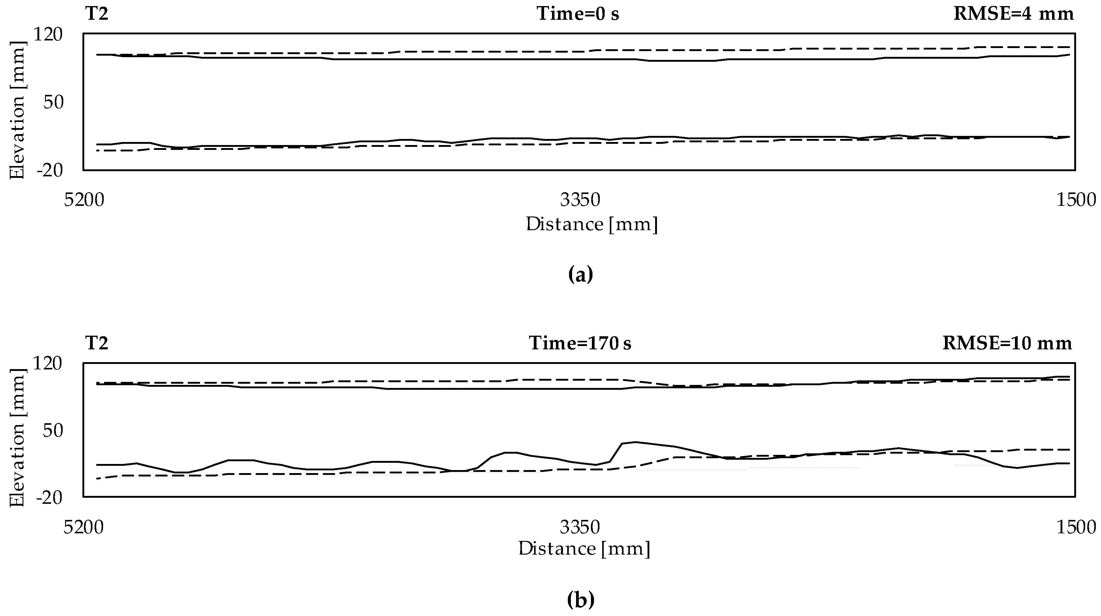
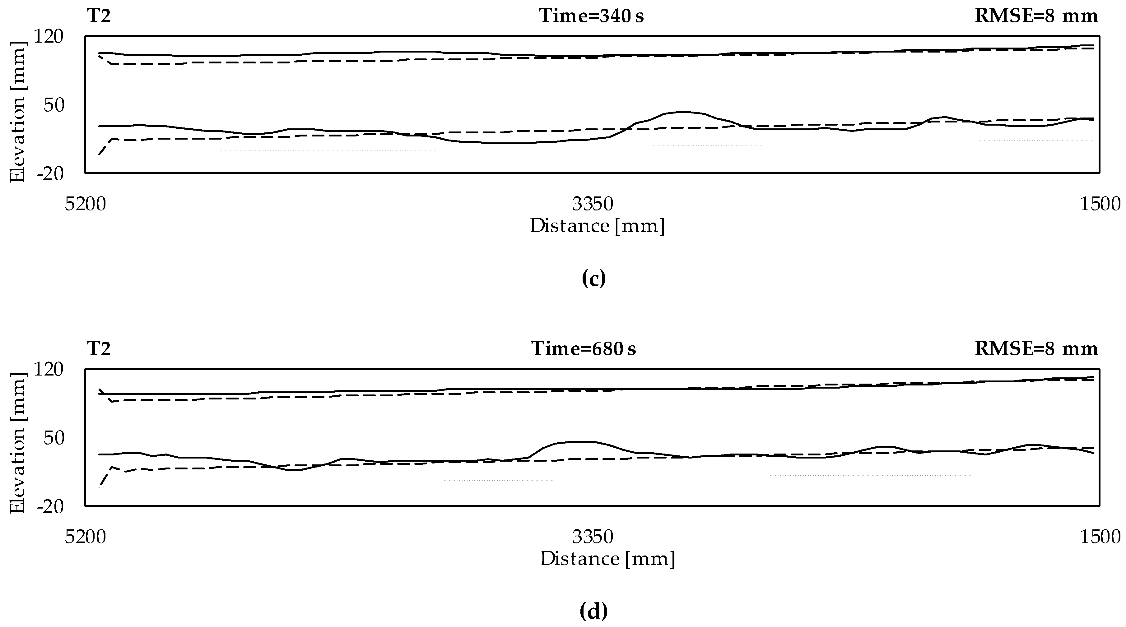
Once calibrated, the numerical model was validated with reference to run T2, that was performed with the same liquid discharge as T1, practically the same sediment feeding rate (0.8% higher) and a downstream water depth that was 15% higher. The experimental (continuous) and numerical (dashed) profiles for run T2 are depicted in Figure 4 and Figure 5. The spatial and temporal evolutions of the bed and water profiles are reproduced quite well also in this case, returning RMSEs values similar to those for run T1 (even though both the water and bed levels tend to be underestimated in the downstream portion of the channel as the experiment proceeds). Finally, an independent validation was also performed by comparing the sediment transport capacity of the downstream sections recorded during run T2 to the one computed by the numerical model. The experimental and numerical values were 1.28 × 10⁻⁵ m3/s and 1.06 × 10⁻⁵ m3/s, respectively (both evaluations are referred to the time elapsed before the arrival of the aggradation front at the downstream of the channel). A relative error of 17.4% was obtained, which was considered encouraging in view of the discrepancies previously observed between the experimental and computed profiles in correspondence of the downstream sections.
3.3. Application of the Calibrated Model to a Transcritical Flow
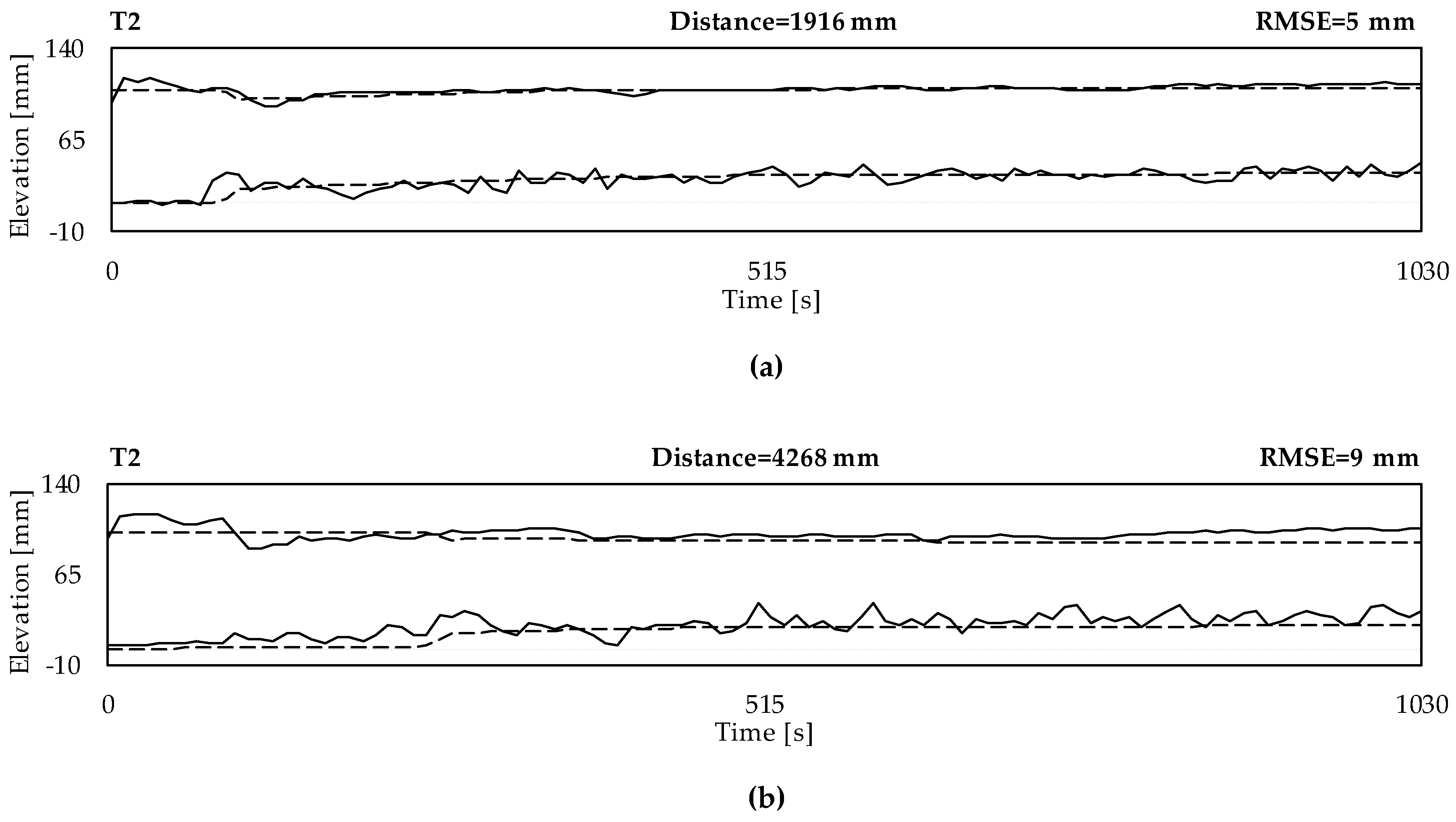
The validated model was also run to simulate test T3, that was performed with a water discharge of 6 l/s, significantly lower than the values for T1 and T2 (14.7 l/s). Run T3 presented a different evolution from runs T1 and T2. In fact, the computation of the Froude number at different locations and times showed that, while T1 and T2 were performed under subcritical flow, a transcritical flow developed during run T3, at some time (variable section by section) after the start of the experiment. Figure 6 presents the temporal evolution of the Froude number at two sections for run T3. The Froude number imposed at the downstream section was 0.66 (Table 1), with similar values taken at both sections of Figure 6 at the beginning of the experiment. After the sediment release, however, the rise of the bed level in the upstream sections caused a change of the water regime from subcritical to supercritical. Furthermore, as the aggradation front propagated, the hydraulic discontinuity also migrated downstream. The flow always remained subcritical at the channel outlet due to the fixed water depth imposed at the last section.
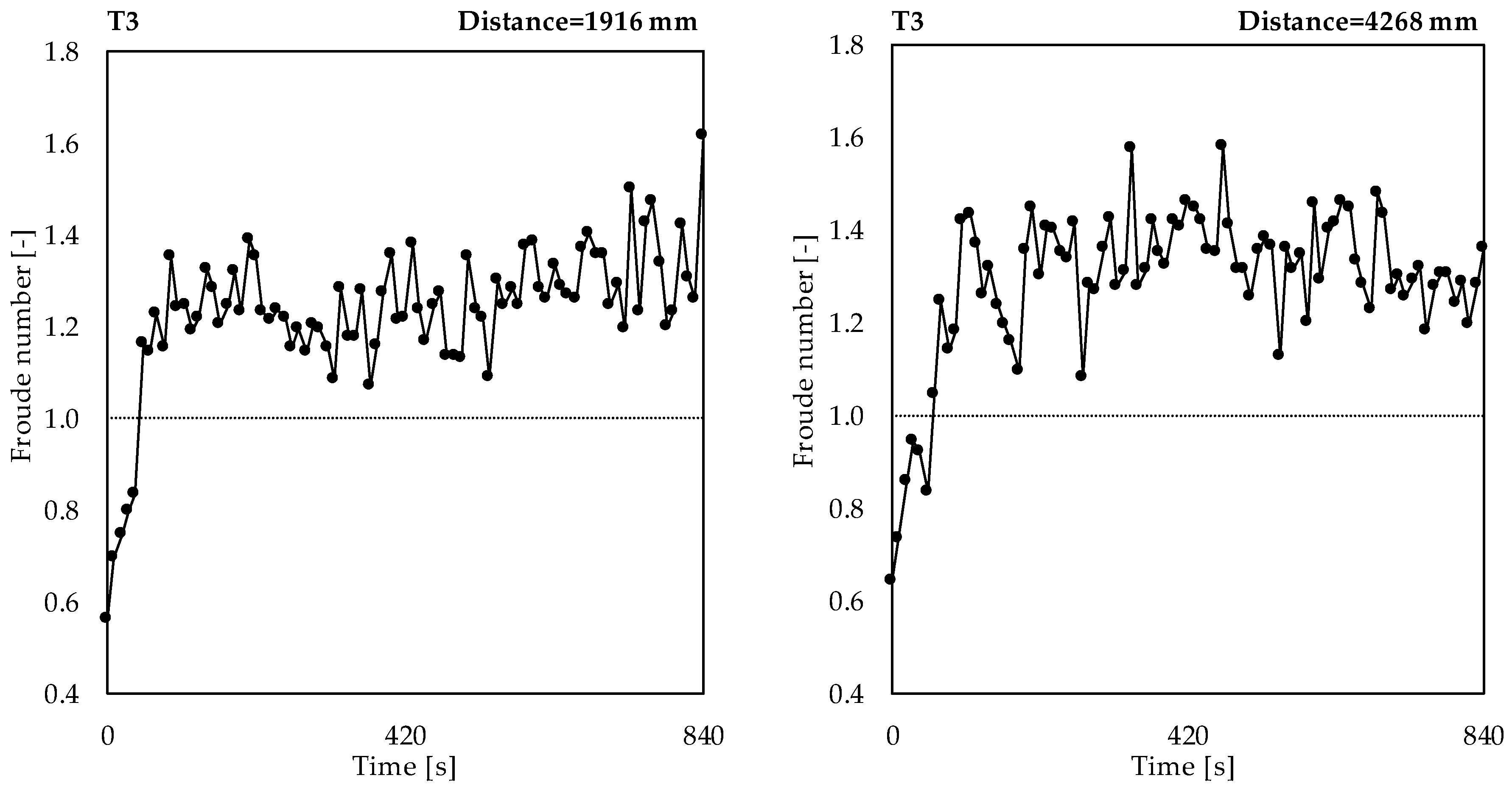
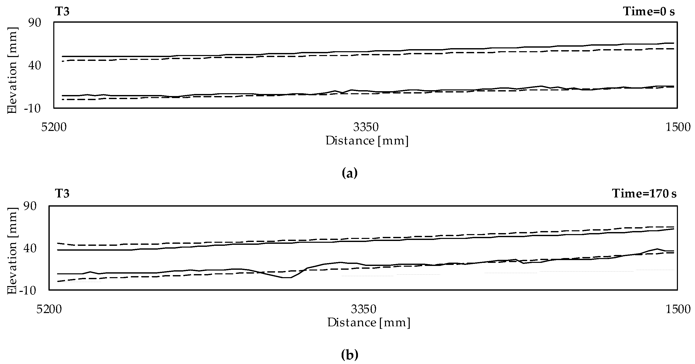
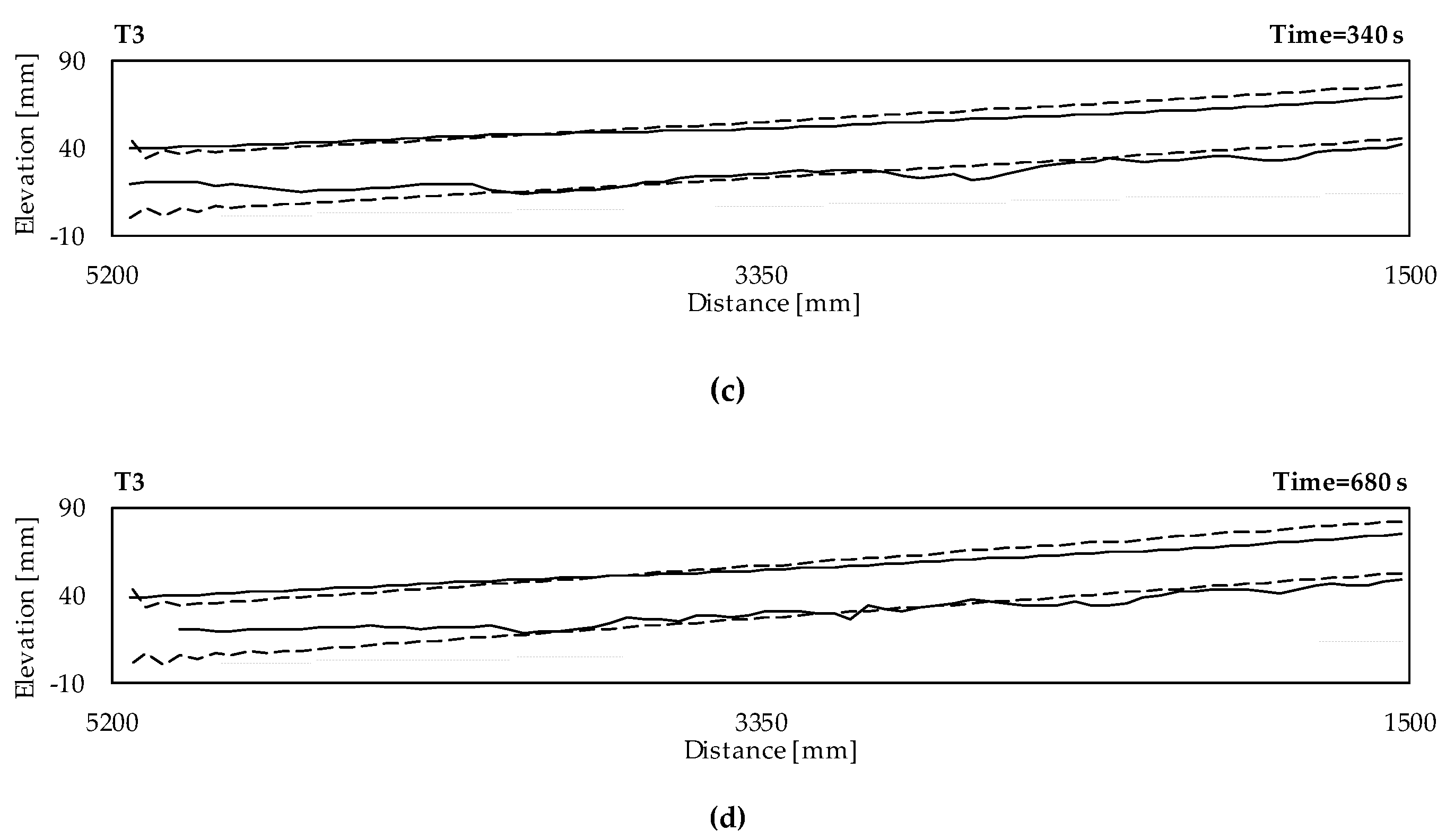
In Figure 7 and Figure 8, some of the obtained experimental (continuous) and numerical (dashed) profiles are depicted. It is evident that, after the sudden rise of the bed level (consequent to the migration of the aggradation front), the program was not able to satisfactorily simulate the spatio-temporal trends of the water and bed surfaces. A mean bed slope much higher than that recorded during run T3 was obtained.
4. Discussion and Conclusions
During all the experimental runs presented in this communication, the sediment overloading caused the development of an aggradation front, which moved downstream as the experiment proceeded, with a consequent gradual increase of the average bed elevation. Moreover, the intense sediment transport led to the formation of dunes.
The mathematical modelling of hydro-morphologic processes by the system (1) requires three boundary conditions. In this work, instead, four boundary conditions were imposed to the numerical model, for Q and zB (through a QBin) at the upstream section, and for h and zB at the downstream one. On the one hand, the number of conditions differs from that required to solve the Saint-Venant–Exner equations (1); on the other hand, these boundary conditions corresponded to the experimental controls (water and sediment feeding rates imposed upstream, tail-water regulation, and sediment sill downstream).
For subcritical experiments (such as T1 and T2 of the present work), one expects two positive and one negative characteristic lines [38]; the downstream boundary condition for zB should not be able to influence the process, and this was indeed observed in both the experimental and numerical runs.
For a supercritical flow, the two positive characteristic lines would be associated with the flow rate and water depth at the inlet (as in clear-water flows), while the negative would be associated to the bed elevation downstream. If the flow becomes trans-critical (like in out experiment T3), some inconsistencies emerge for how the conditions had to be posed in the present work: (i) an upstream condition for the water depth was missing; (ii) the upstream condition for zB (through QBin) should have become ineffective, but this was not observed experimentally nor numerically; (iii) the downstream condition for zB started to influence the numerical results (even if it should not have to) while it did not influence the experimental ones. On the one hand, some morphologic change may be propagated upstream and downstream also by changes in the water profile. On the other hand, the above were possibly the reasons for which the numerical model gave unsatisfactory results when applied to T3. In the literature, it has been argued that trans-critical flows with a mobile bed can be handled by a conventional numerical approach [39] and examples of numerically simulated mixed-flow regime can be found [40,41]. However, most of the discussed case studies deal with conditions remaining constant at the boundaries while, to the best of our knowledge, the numerical modelling of a trans-critical flow in both space and time was only performed by Reference [40]. The study focused on the response of a channel bed to the presence of a hydraulic jump. The flow was initially supercritical along the entire channel length. This equilibrium situation was perturbed by the rapid rise of a submerged weir at the downstream end of the flume, which determined a subcritical flow at the downstream, a hydraulic discontinuity and a sediment front. This experiment was designed ensuring that the boundary conditions were appropriately posed before and after the flow transition.
Our analysis supports the conclusion that transient flows can be numerically modelled knowing the instant at which the water regime changes; numerical models with different sets of boundary conditions may be run before and after this time (even though this strategy was not applied to the present experiment T3).
Author Contributions
All the authors conceived and designed the study and ran the experiments; B.Z. and M.Z. processed the experimental data; B.Z. and M.Z. ran the numerical simulations; all the authors contributed to the discussion of the results; B.Z. wrote the paper, that was then revised by all the authors.
Funding
This research was partially supported by Fondazione Cariplo (Italy) through the project entitled Sustainable Management of Sediment Transport in Response to Climate Change Conditions (SMART-SED).
Conflicts of Interest
The authors declare no conflict of interest.
References
- Lane, S.N.; Tayefi, V.; Reid, S.C.; Yu, D.; Hardy, R.J. Interactions between sediment delivery, channel change, climate change and flood risk in a temperate upland environment. Earth Surf. Proc. Land. 2007, 32, 429–446. [Google Scholar] [CrossRef] [Green Version]
- Dotterweich, M. The history of soil erosion and fluvial deposits in small catchments of central Europe: Deciphering the long-term interaction between humans and the environment—A review. Geomorphology 2008, 101, 192–208. [Google Scholar] [CrossRef]
- Neuhold, C.; Stanzel, P.; Nachtnebel, H.P. Incorporating river morphological changes to flood risk assessment: Uncertainties, methodology and application. Nat. Hazards Earth Syst. Sci. 2009, 9, 789–799. [Google Scholar] [CrossRef]
- Verhaar, P.M.; Biron, P.M.; Ferguson, R.I.; Hoey, T.B. Implications of climate change in the twenty-first century for simulated magnitude and frequency of bed-material transport in tributaries of the Saint-Lawrence River. Hydrol. Process. 2011, 25, 1558–1573. [Google Scholar] [CrossRef]
- Radice, A.; Giorgetti, E.; Brambilla, D.; Longoni, L.; Papini, M. On integrated sediment transport modeling for flash events in mountain environments. Acta Geophys. 2012, 60, 191–213. [Google Scholar] [CrossRef]
- Radice, A.; Rosatti, G.; Ballio, F.; Franzetti, S.; Mauri, M.; Spagnolatti, M.; Garegnani, G. Management of flood hazard via hydro-morphological river modelling. The case of the Mallero in Italian Alps. J. Flood Risk Manag. 2013, 6, 197–209. [Google Scholar] [CrossRef]
- de Miranda, R.B.; Mauad, F.F. Influence of sedimentation on hydroelectric power generation: Case study of a Brazilian reservoir. J. Energy Eng. 2014, 141, 04014016. [Google Scholar] [CrossRef]
- Pender, D.; Patidar, S.; Hassan, K.; Haynes, H. Method for incorporating morphological sensitivity into flood inundation modeling. J. Hydraul. Eng. 2016, 142, 04016008. [Google Scholar] [CrossRef]
- Wharton, G.; Mohajeri, S.H.; Righetti, M. The pernicious problem of streambed colmation: A multi-disciplinary reflection on the mechanisms, causes, impacts, and management challenges. WIREs Water 2017, 4, e1231. [Google Scholar] [CrossRef]
- Parsapour-Moghaddam, P.; Rennie, C.D. Influence of meander confinement on hydro-morphodynamics of a cohesive meandering channel. Water 2018, 10, 354. [Google Scholar] [CrossRef]
- Krysanova, V.; Hattermann, F.; Wechsung, F. Development of the ecohydrological model SWIM for regional impact studies and vulnerability assessment. Hydrol. Process. 2005, 19, 763–783. [Google Scholar] [CrossRef]
- Coulthard, T.J.; Macklin, M.G.; Kirkby, M.J. A cellular model of Holocene upland river basin and alluvial fan evolution. Earth Surf. Proc. Land. 2002, 27, 269–288. [Google Scholar] [CrossRef]
- Kim, J.; Ivanov, V.Y.; Katopodes, N.D. Modeling erosion and sedimentation coupled with hydrological and overland flow processes at the watershed scale. Water Resour. Res. 2013, 49, 5134–5154. [Google Scholar] [CrossRef] [Green Version]
- Wright, S.A.; Topping, D.J.; Rubin, D.R.; Melis, T.S. An approach for modeling sediment budgets in supply-limited rivers. Water Resour. Res. 2010, 46, W10538. [Google Scholar] [CrossRef]
- Radice, A.; Longoni, L.; Papini, M.; Brambilla, D.; Ivanov, V.I. Generation of a design flood-event scenario for a mountain river with intense sediment transport. Water 2016, 8, 597. [Google Scholar] [CrossRef]
- Papanicolaou, A.N.; Bdour, A.; Wicklein, E. One-dimensional hydrodynamic/sediment transport model applicable to steep mountain streams. J. Hydraul. Res. 2004, 42, 357–375. [Google Scholar] [CrossRef]
- Chiari, M.; Friedl, K.; Rickenmann, D. A one-dimensional bedload transport model for steep slopes. J. Hydraul. Res. 2010, 48, 152–160. [Google Scholar] [CrossRef]
- Rosatti, G.; Bonaventura, L.; Deponti, A.; Garegnani, G. An accurate and efficient semi-implicit method for section-averaged free-surface flow modeling. Int. J. Numer. Meth. Fluids 2011, 65, 448–473. [Google Scholar] [CrossRef]
- Viparelli, E.; Haydel, R.; Salvaro, M.; Wilcock, P.R.; Parker, G. River morphodynamics with creation/consumption of grain size stratigraphy 1: Laboratory experiments. J. Hydraul. Res. 2010, 48, 715–726. [Google Scholar] [CrossRef]
- Viparelli, E.; Sequeiros, O.E.; Cantelli, A.; Wilcock, P.R.; Parker, G. River morphodynamics with creation/consumption of grain size stratigraphy 2: Numerical model. J. Hydraul. Res. 2010, 48, 727–741. [Google Scholar] [CrossRef]
- Soni, J.P.; Garde, R.J.; Ranga Raju, K.G. Aggradation in streams due to overloading. ASCE J. Hydraul. Div. 1980, 106, 117–132. [Google Scholar]
- Soni, J.P. Laboratory study of aggradation in alluvial channels. J. Hydrol. 1981, 49, 87–106. [Google Scholar] [CrossRef]
- Yen, C.L.; Chang, S.Y.; Lee, H.Y. Aggradation-degradation process in alluvial channels. J. Hydraul. Eng. 1992, 118, 1651–1669. [Google Scholar] [CrossRef]
- Alves, E.; Cardoso, A. Experimental study on aggradation. Int. J. Sediment Res. 1999, 14, 1–15. [Google Scholar]
- Miglio, A.; Gaudio, R.; Calomino, F. Mobile-bed aggradation and degradation in a narrow flume: Laboratory experiments and numerical simulations. J. Hydro-Environ. Res. 2009, 3, 9–19. [Google Scholar] [CrossRef]
- Unigarro Villota, S. Laboratory Study of Channel Aggradation due to Overloading. Master’s Thesis, Politecnico di Milano, Milan, Italy, December 2017. [Google Scholar]
- Zanchi, B. Indagine Sperimentale Sul Fenomeno di Deposito in un Canale a Fondo Mobile Sovralimentato. Master’s Thesis, Politecnico di Milano, Milan, Italy, July 2018. (In Italian). [Google Scholar]
- Radice, A.; Unigarro Villota, S. Propagation of aggrading sediment fronts in a laboratory flume. In Proceedings of the River Flow 2018, Lyon, France, 5–8 September 2018. [Google Scholar]
- Zucchi, M. Experimental and Numerical Study of Channel Aggradation. Master’s Thesis, Politecnico di Milano, Milan, Italy, December 2018. [Google Scholar]
- Radice, A.; Zanchi, B. Multicamera, multimethod measurements for hydromorphologic laboratory experiments. Geosciences 2018, 8, 172. [Google Scholar] [CrossRef]
- Graf, H.W.; Altinakar, M.S. Fluvial Hydraulics. Flow and Transport Processes in Channels of Simple Geometry; Wiley: Chichester, UK, 1998. [Google Scholar]
- Strickler, A. Beitraege zur Frage der Geschwindigkeitsformel und der Rauhigkeitszahlen Fuer Stroeme, Kanaele und Geschlossene Leitungen; Mitteilungen des Amtes fuer Wasserwirtschaft; Eidgenoessisches Departement des Innern: Bern, Switzerland, 1923; Volume 16. (In German) [Google Scholar]
- Meyer-Peter, E.; Müller, R. Formulas for Bed-Load Transport; Report on the Second IAHR Meeting, Stockholm, Sweden; TU Delft: Delft, The Netherlands, 1948; pp. 39–64. [Google Scholar]
- Shields, A. Anwendung der aehnlichkeitsmechanik und der turbulenz forschung auf die geschiebebewegung. In Mitteilungen der Preussische Versuchanstalt für Wasserbau und Schiffsbau Heft 26; TU Delft: Berlin, Germany, 1936. (In German) [Google Scholar]
- Van Rijn, L.C. Sediment transport, part II: Suspended load transport. J. Hydraul. Eng. 1984, 110, 1613–1641. [Google Scholar] [CrossRef]
- Vetsch, D.; Siviglia, A.; Caponi, F.; Ehrbar, D.; Gerke, E.; Kammerer, S.; Koch, A.; Peter, S.; Vanzo, D.; Vonwiller, L.; et al. System manuals of BASEMENT, version 2.8; Laboratory of Hydraulics, Glaciology and Hydrology (VAW), ETH Zurich: Zurich, Switzerland, 2018. [Google Scholar]
- Roe, P.L. Approximate Riemann solvers, parameter vectors and difference schemes. J. Comput. Phys. 1981, 43, 357–372. [Google Scholar] [CrossRef]
- Armanini, A. Principi di Idraulica Fluviale; Editoriale Bios: Cosenza, Italy, 2002. (In Italian) [Google Scholar]
- Lyn, D.A.; Altinakar, M. St. Venant–Exner equations for near-critical and transcritical flows. J. Hydraul. Eng. 2002, 128, 579–587. [Google Scholar] [CrossRef]
- Goutière, L.; Soares-Frazão, S.; Savary, C.; Laraichi, T.; Zech, Y. One-dimensional model for transient flows involving bed-load sediment transport and changes in flow regimes. J. Hydraul. Eng. 2008, 134, 726–735. [Google Scholar] [CrossRef]
- Bellal, M.; Spinewine, B.; Savary, C.; Zech, Y. Morphological evolution of steep-sloped river beds in the presence of a hydraulic jump: Experimental study. In Proceedings of the 30th IAHR Congress, Thessaloniki, Greece, 25–31 August 2003. [Google Scholar]
Figure 1.
Schematic representation of the laboratory facility.

Figure 2.
Longitudinal bed and water profiles for the experiment T1 obtained experimentally (continuous) and numerically (dashed) at (a) 0 s, (b) 170 s, (c) 340 s, and (d) 680 s. The horizontal axis represents the stream-wise distance from the inlet, whereas the vertical coordinates were measured with respect to the initial bed surface elevation at the channel outlet. The longitudinal bed profile at 0 s is represented by the gray line. Flow is from right to left.


Figure 3.
Temporal evolution of bed and water profiles for the experiment T1 obtained experimentally (continuous) and numerically (dashed) at about (a) 1.9 m and (b) 4.3 m from the channel inlet. The time instant 0 s corresponds to the beginning of the sediment release. The vertical coordinates were measured with respect to the initial bed surface elevation at the channel outlet. The initial bed level is indicated by the gray line.

Figure 4.
Longitudinal bed and water profiles for the experiment T2 obtained experimentally (continuous) and numerically (dashed) at (a) 0 s, (b) 170 s, (c) 340 s, and (d) 680 s. The horizontal axis represents the stream-wise distance from the inlet, whereas the vertical coordinates were measured with respect to the initial bed surface elevation at the channel outlet. The longitudinal bed profile at 0 s is represented by the gray line. Flow is from right to left.


Figure 5.
Temporal evolution of bed and water profiles for the experiment T2 obtained experimentally (continuous) and numerically (dashed) at about (a) 1.9 m and (b) 4.3 m from the channel inlet. The time instant 0 s corresponds to the beginning of the sediment release. The vertical coordinates were measured with respect to the initial bed surface elevation at the channel outlet. The initial bed level is indicated by the gray line.

Figure 6.
Temporal evolution of the Froude number at two different locations along the channel during the aggradation test T3.
Figure 6.
Temporal evolution of the Froude number at two different locations along the channel during the aggradation test T3.

Figure 7.
Longitudinal bed and water profiles for the experiment T3 obtained experimentally (continuous) and numerically (dashed) at (a) 0 s, (b) 170 s, (c) 340 s, and (d) 680 s. The horizontal axis represents the stream-wise distance from the inlet, whereas the vertical coordinates were measured with respect to the initial bed surface elevation at the channel outlet. The longitudinal bed profile at 0 s is represented by the gray line. Flow is from right to left.


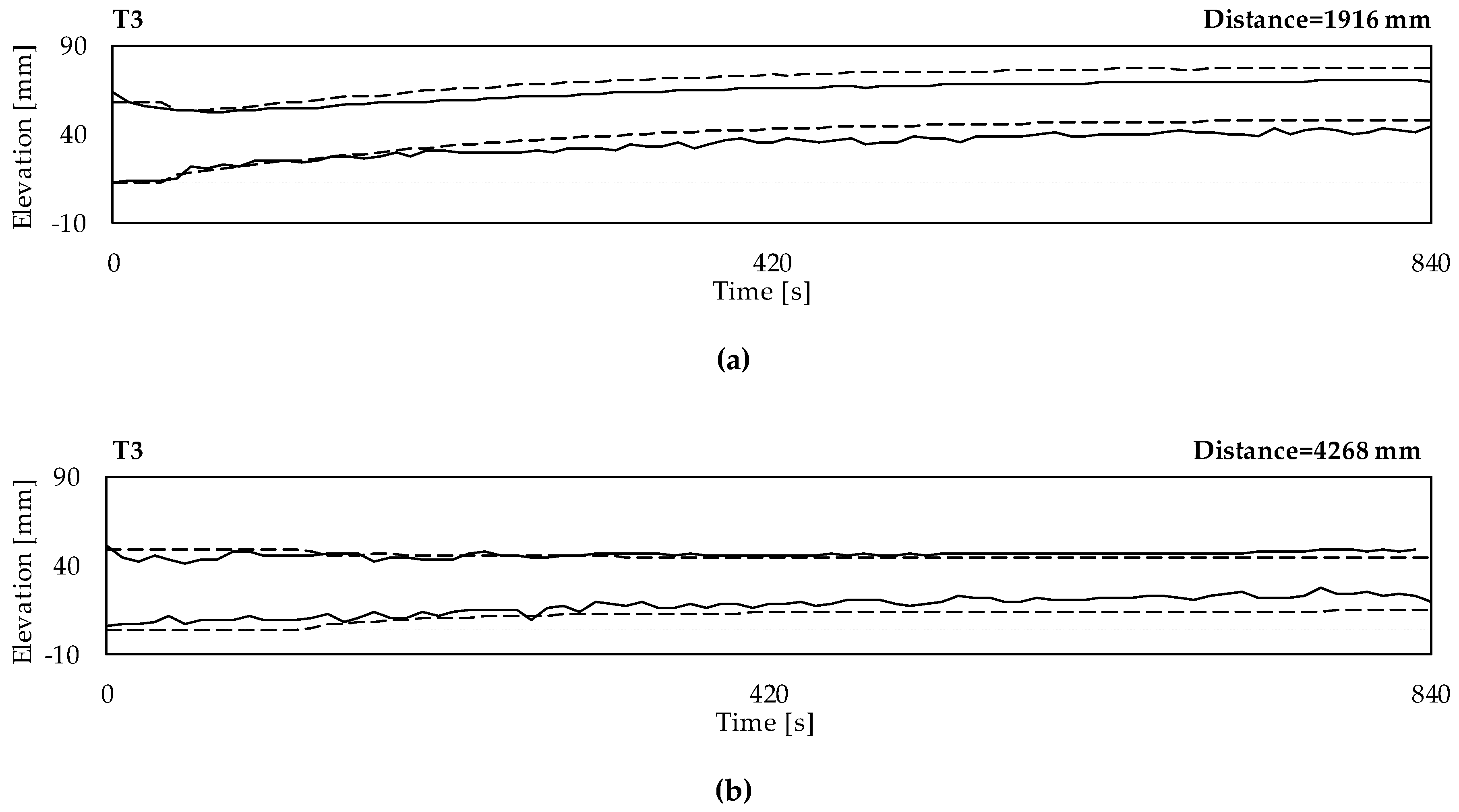
Figure 8.
Temporal evolution of bed and water profiles for the experiment T3 obtained experimentally (continuous) and numerically (dashed) at about (a) 1.9 m and (b) 4.3 m from the channel inlet. The time instant 0 s corresponds to the beginning of the sediment release. The vertical coordinates were measured with respect to the initial bed surface elevation at the channel outlet. The initial bed level is indicated by the gray line.


Table 1.
Main parameters of the aggradation experiments.
| T [s] | Q [l/s] | hd [cm] | h0 [cm] | Ud [m/s] | Frd [–] | QBin [10−5 m3/s] | |
|---|---|---|---|---|---|---|---|
| T1 | 936 | 14.7 | 8.6 | 8.3 | 0.57 | 0.62 | 5.51 |
| T2 | 1113 | 14.7 | 9.9 | 8.3 | 0.50 | 0.51 | 5.55 |
| T3 | 845 | 6.0 | 4.5 | 4.5 | 0.44 | 0.66 | 7.43 |
© 2019 by the authors. Licensee MDPI, Basel, Switzerland. This article is an open access article distributed under the terms and conditions of the Creative Commons Attribution (CC BY) license (http://creativecommons.org/licenses/by/4.0/).
Share and Cite
MDPI and ACS Style
Zanchi, B.; Zucchi, M.; Radice, A. On the Relationship between Experimental and Numerical Modelling of Gravel-Bed Channel Aggradation. Hydrology 2019, 6, 9. https://doi.org/10.3390/hydrology6010009
AMA Style
Zanchi B, Zucchi M, Radice A. On the Relationship between Experimental and Numerical Modelling of Gravel-Bed Channel Aggradation. Hydrology. 2019; 6(1):9. https://doi.org/10.3390/hydrology6010009
Chicago/Turabian StyleZanchi, Barbara, Matteo Zucchi, and Alessio Radice. 2019. "On the Relationship between Experimental and Numerical Modelling of Gravel-Bed Channel Aggradation" Hydrology 6, no. 1: 9. https://doi.org/10.3390/hydrology6010009
Note that from the first issue of 2016, this journal uses article numbers instead of page numbers. See further details here.