Deterministic Methodology for Determining the Optimal Sampling Frequency of Water Quality Monitoring Systems

Abstract

This paper proposes a novel deterministic methodology for estimating the optimal sampling frequency (SF) of water quality monitoring systems. The proposed methodology is based on employing two-dimensional contaminant transport simulation models to determine the minimum SF, taking into consideration all the potential changes in the boundary conditions of a water body. Two-dimensional contaminant transport simulation models (RMA4) were implemented to estimate the distribution patterns of some effective physiochemical parameters within the Al-Hammar Marsh in the southern part of Iraq for 30 cases of potential boundary conditions. Using geographical information system (GIS) tools, a spatiotemporal analysis approach was applied to the results of the RMA4 models to determine the minimum SF of the monitoring stations with a monitoring accuracy (MA) level of detectable change in contaminant concentration ranging from the standard level to 50% (stepwise 5%). For the study area, the proposed methodology specified a minimum and maximum SF for each monitoring station (MS) that ranged between 12 and 33 times per year, respectively. An exponential relationship between SF and MA was obtained. This relationship shows that increasing the MA to ±10%, ±25%, and ±50% increases the SF by approximately 14%, 28%, and 93%, respectively. However, the proposed methodology includes all the potential values and cases of flow and contaminant transport boundary conditions, which increases the certainty of monitoring the system and the efficiency of the SF schedule. Moreover, the proposed methodology can be effectively applied to all types of surface water resources.

1. Introduction

Water pollution is a growing menace to natural ecosystems and human life. The distribution of pollution within a water resource system is characterized by significant spatial and temporal variations due to differences in hydrological conditions and pollution sources. Overcoming this challenge requires a better understanding of the spatial and temporal variations in the distribution of contaminants within aquatic systems [1]. An efficient assessment of the water quality (WQ) within a water resource system is highly dependent on the efficiency of the monitoring network (MN). However, obtaining the optimal design of water quality monitoring networks (WQMNs) is a very complex process due to the large number of factors that must be considered, such as monitoring objectives, water quality parameters, monitoring station locations, and sampling frequency (SF) [2]. Accordingly, SF is a very important variable in the design of WQMNs. An appropriate SF ensures that no pollution surge passes a monitoring station (MS) without being detected. The design aspects of WQMNs have been widely considered since the 1940s [2]. Additionally, the optimal design of a WQMN, taking into consideration the SF and all issues related to the improvement of monitoring program efficiency, has been widely addressed in the literature [3,4]. After the 1980s, many attempts were carried out to improve monitoring efficiency with regard to the problem constraints and design criteria [5,6,7]. Subsequently, the optimal design of WQMNs was discussed in [8], and the basic principles of WQMN design and criteria of allocating WQMSs were applied in [9,10,11,12]. Thereafter, many studies in the 1990s covered topics concerned with specifying the SF, such as [13,14,15,16,17,18]. Moreover, integer programming and multi-objective programming, in which more complex issues were addressed, were used to assess the SF [19,20,21]. A comprehensive review of these papers can be found in [22]. Reference [23] presented sampling frequencies for the Global Environment Monitoring System for freshwater (GEMS/Water) baseline and trend stations, as shown in

Table 1. Sampling frequency for Global Environment Monitoring System for freshwater (GEMS/WATER) stations [23].

Water Body		Sampling Frequency
Baseline stations	Streams	Minimum: four per year, including high- and low-water stages. Optimum: 24 per year (every second week); weekly for total suspended solids.
	Headwater lakes	Minimum: one per year at turnover; sampling at lake outlet. Optimum: one per year at turnover, and one vertical profile at the end of stratification season.
Trend stations	Rivers	Minimum: 12 per year for large drainage areas (approximately 100,000 km2). Maximum: 24 per year for small drainage areas (approximately 10,000 km2).
	Lakes and reservoirs	For issues other than eutrophication: Minimum: one per year at turnover. Maximum: two per year at turnover, and one at maximum thermal stratification. For eutrophication: 12 per year, including twice monthly during the summer.
	Groundwater	Minimum: one per year for large, stable aquifers. Maximum: four per year for small, alluvial aquifers. Karst aquifers: same as rivers.

.

The effective design of a WQMN was considered using various types of statistical and/or programming techniques, such as integer programming, multi-objective programming, kriging theory, and optimization analysis [14,19,20,21,24,25]. Additionally, statistical approaches used for the assessment and redesign of WQMNs were reviewed by [26]. In this review, various monitoring objectives and related assessment and redesign methods of long-term WQMNs were discussed. Based on the pollution level to be detected and variability of the WQ data, a statistical approach is commonly used to estimate the WQ SF [27]. The statistical tools that are commonly used to optimize the temporal frequency of monitoring in WQ networks are confidence intervals, trend analyses, geostatistical tools, multivariate analyses, optimization programs, entropy analyses, and artificial neural networks [26]. Two quantitative measures of the effectiveness of different sampling frequencies were proposed by [7]. These measures are destined to be utilized at the preliminary design stage to detect violations of WQ standards. The analytic hierarchy process (AHP), which is an effective method for decision analysis, was applied to analyze environmental impact assessments [28] and design river WQ SF [29].

In recent years, computer-aided mathematical simulation models of water quality have been rapidly developed [30]. Such models can be used to predict water quality by accounting for changes that affect water quality factors or changes in their intensity. Two-dimensional models (2D) are used most often in the case of lakes, reservoirs, or deep rivers. The end result of these models is an estimation of water quality parameters close to measurements of actual concentrations. The assessment of individual parameters can be performed for given time intervals: hourly, daily, weekly, monthly, and yearly [31]. Integral utilization of simulation models and the tools and facilities of geographical information systems (GIS) can assist and support developing new efficient approaches to obtain the optimal design of a WQMN.

However, a comprehensive review of the abovementioned literature showed that WQMNs have traditionally been designed on the basis of a measured dataset collected from nonoptimal preallocated monitoring stations (MSs). Additionally, an assessment of the monitoring efficiency of the stations of a WQMN was implemented using statistical methods and general criteria. These methods and criteria were applied to insufficient datasets because some effective events or values, which are required for achieving the monitoring objectives, may not be detected because of the inadequacy of the locations and SFs of the MSs. Consequently, the obtained level of monitoring accuracy was based on the number of detected events according to these MSs, which does not account for all the events that have occurred or the potential of future events. Moreover, the effects of changes in boundary conditions, land cover, and land use on optimal SF were not taken into consideration. The update, reanalysis, reassessment, and reuse of a WQMN database using the traditional method are very difficult.

This paper aims to present a new deterministic approach for employing the features and facilities of the hydrodynamic simulation models of contaminants transport to specify the optimal SF for each MS in the WQMN according to all potential changes in the boundary conditions of a water body. Furthermore, maximizing the monitoring accuracy of each MS and subsequently the overall WQMN decreases the cost, time, and effort of monitoring. The methodology of obtaining the optimal SF should start with specifying the optimal locations of MSs. However, many authors previously considered this stage. Specifically, for the Al-Hammar Marsh, which is the study area in this research, the optimal locations of MSs (46 stations) were specified by Al-Khafaji, and Abdulraheem [32]. Therefore, the optimal allocation of the MS was not considered as an aim of this study. This paper concerns specifying the SF schedule for prespecified optimal locations of MSs in a WQMN.

2. Materials and Methods

2.1. Methodology

The computation of SF is based on specifying the minimum interval between successive detectable changes in the value or concentration of a WQ parameter at an MS. However, the SF must be sufficient to detect the change in WQ within an accuracy level specified according to the monitoring objectives. This SF must ensure the detection of the entire pollution surges that pass an MS. This MS should be located at the optimal position where it is most sensitive to changes in the WQ.

The WQ distribution patterns and the velocity and time of contaminant transport can be estimated by using hydrodynamic and contaminant transport simulation models. Two-dimensional simulation models are sufficient tools for studying the transport of contaminants within lakes, reservoirs, or deep rivers [31].

The time scale of the SF is usually greater than one day. Additionally, the differences in the diffusion velocities of contaminants caused by the variations in the diffusion and dispersion coefficients in most water bodies, such as marshes, which usually have low flow velocity in comparison to most lakes and rivers, are not large enough to make a difference in the transport time of the contaminants between the MSs greater than one day. Therefore, it was not necessary to include all the WQ parameters for specifying the optimal SF. Hence, some of the major effective WQ parameters can be used as indicators to give comprehensive representation for the WQ. Consequently, some effective physiochemical parameters (total dissolved solids (TDS), turbidity, acidity (pH), total hardness (TH), dissolved oxygen (DO), and biological oxygen demand (BOD), Ca²⁺, Mg²⁺, Na⁺, SO₄²⁻, PO₄³⁻ and NO3⁻, Cd, Cr, and Pb) were selected based on the available data Accordingly, the required level of WQ parameters monitoring accuracy (the detectable change in contaminant concentration) could be adopted as the required level of monitoring accuracy (MA) at the MSs. The recommended accuracy (uncertainty levels) expressed at the 95% confidence interval is ± 5% [33]. Consequently, the minimum interval of SF in an MS should be the minimum time interval between two successive ± 5% changes in contaminant concentration.

When there is a large number of spatially relevant data, the spatial analysis tools of geographical information systems (GIS) can be utilized to address such data. Therefore, these tools could be employed to determine the SF of all the WQ MSs within the study area.

Accordingly, the proposed approach was based on utilizing two-dimensional hydrodynamic and contaminant transport simulation models to compute the WQ distribution patterns, taking into consideration all the potential changes in the boundary conditions of a water body. Subsequently, a spatiotemporal analysis approach was applied to the results of the contaminant transport models using geographical information system (GIS) tools to determine the minimum SF of the monitoring stations, with a monitoring accuracy (MA) level of detectable change in contaminant concentration ranging from the standard level to 50% (stepwise 5%).

The methodology of the proposed approach can be summarized as follows:

• The study area was specified and the topography data of the study area was collected, including locations of the preallocated MSs of the considered WQMN and recorded discharge, water depth and WQ datasets at the inlet, outlet, and within the water body;
• The hydraulic and WQ datasets were analyzed, in this research they were some effective physiochemical parameters (TDS, Ph, Turbidity, TH, DO, and BOD, Ca²⁺, Mg²+, Na+, SO₄²⁻, PO₄³⁻ and NO3⁻Cd, Cr, and Pb), to specify all the potential cases and values of the boundary conditions for the study area. Consequently, the required calibration and verification datasets were specified according to these cases;
• The hydrodynamic and contaminant transport simulation models were implemented. Before applying these models for all potential cases of boundary conditions, the calibration and verification processes were performed;
• Based on the results of the contaminant transport simulation model, the spatiotemporal analysis tools of GIS were utilized to obtain the temporal changes in the considered WQ parameters distribution patterns within the considered water body. Subsequently, the minimum time interval of detecting a successive change in the concentration of the considered WQ parameters was computed at each MS with MA of each WQ parameter for each case of boundary conditions;
• To evaluate the effect of changing the MA, the results of the contaminants transport simulation models (for each WQ parameters) were reanalyzed using the spatiotemporal analysis approach and increasing the MA from ±5% to ±50% (stepwise 5%) for each WQ parameter for each case of boundary conditions;
• To verify the proposed methodology, a sampling schedule was implemented based on the criteria of the sampling frequency for GEMS/WATER stations UNEP/WHO [23] to compare with the results produced by using the proposed methodology;
• The results were analyzed and discussed, and the main conclusions and recommendations were presented.

2.2. Study Area

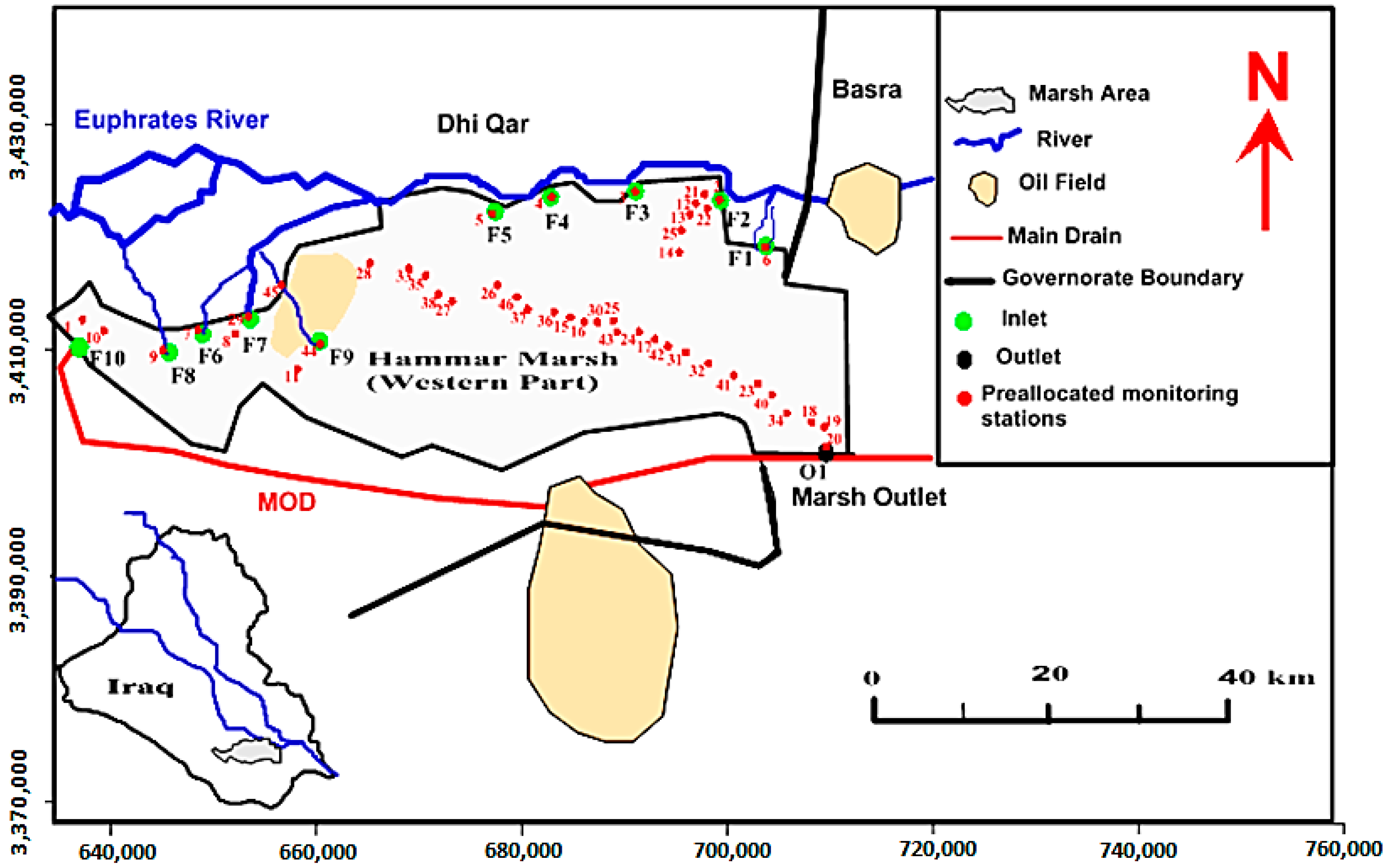
The western part of the Al-Hammar Marsh is located within the southeastern part of the Thi-Qar Governorate in southern Iraq (Figure 1). The Al-Hammar Marsh has an area of approximately 1350 km² and a maximum water depth of 1.8 m a.s.l. The marsh has a complex feeding and outlet system. Some of the marsh feeders, which were denoted BC3 (F1), FBC3 (F 2), FW (F3), FBC4 (F4), and BC4 (F5) are short channels that convey the water directly from the Euphrates River to the marsh. These feeders work as feeders and/or outlets according to the levels of the water surface in the marsh and Euphrates River. In contrast, other feeders, such as Um Nakhla (F6), Al-Kurmashia (F7), Al-Qausy Drain (F8), and Al-Hamedy (F9), convey the water from a reach of the Euphrates River upstream of the marsh to the western zone of the marsh. Additionally, some of the main outfall drain (MOD) water is discharged into the marsh through the Al-Khamissiya Canal (F10). The main outlet of the marsh is the Al-Hammar Outlet (O1), which is located downstream of the eastern zone of the marsh.

The marsh boundary and locations of the preallocated WQ MSs (46 stations) for this part of the Al-Hammar Marsh were specified by Al-Khafaji and Abdulraheem [32], as shown in Figure 1.

A digital elevation model (DEM) for the study area, shown in Figure 2, was created by using the topographical survey data provided by the General Directorate of Survey/MoWR in May 2017 (unpublished data).

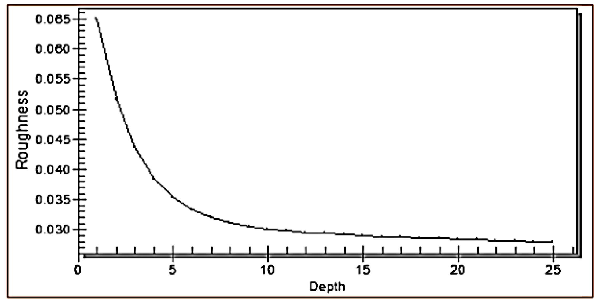
Alhamdani [34] obtained and verified the roughness–depth relationship of the marsh bed given by Manning’s roughness coefficients, as shown in Figure 3. The annual average evapotranspiration (ETo) of the marsh is 2909.3 mm, according to [35].

The Center for the Restoration of Iraqi Marsh and Wetland (CRIMW) provided the recorded discharge, water surface elevation, and most of required data of considered physiochemical parameters at the inlet, outlet, and within the marsh for the period of 2010 to 2017 (unpublished data). Additionally, other datasets (missing), were completed from [36,37]. These datasets were analyzed to specify the potential cases and values of the marsh boundary conditions for the water quantity and quality aspects. According to the requirements of the hydrodynamic and contaminant transport simulation models, these boundary conditions can be represented by 30 cases. However, because of manuscript size limitations, for WQ parameters, only the TDS concentration was shown (see

Table 2. Potential cases of marsh boundary conditions for the hydrodynamic simulation model (CRIMW 2017 (unpublished data)).

Case No.	Discharge (m3/sec)										WSE (m a.s.l.)
	BC3	BC4	FBC3	FBC4	FW	Um Nakhla	Al-Kurmashia	Al-Qausy Drain	Al-Hamedy	Al-Khamissiya	Hammar Outlet
1	3.93	3.83	4.60	5.50	10.00	6.85	3.85	29.63	5.30	56.55	1.90
2	3.93	3.83	4.60	5.50	10.00	6.85	3.85	29.63	5.30	26.38	1.90
3	3.93	3.83	4.60	5.50	10.00	6.85	3.85	29.63	5.30	9.70	1.90
4	1.82	2.19	1.87	1.95	2.08	3.14	1.76	13.25	1.97	56.55	1.90
5	1.82	2.19	1.87	1.95	2.08	3.14	1.76	13.25	1.97	26.38	1.90
6	1.82	2.19	1.87	1.95	2.08	3.14	1.76	13.25	1.97	9.70	1.90
7	0.43	0.50	0.50	0.45	0.35	0.85	0.35	3.00	0.20	56.55	1.90
8	0.43	0.50	0.50	0.45	0.35	0.85	0.35	3.00	0.20	26.38	1.90
9	0.43	0.50	0.50	0.45	0.35	0.85	0.35	3.00	0.20	9.70	1.90
10	3.93	3.83	4.60	5.50	10.00	6.85	3.85	29.63	5.30	56.55	1.67
11	3.93	3.83	4.60	5.50	10.00	6.85	3.85	29.63	5.30	26.38	1.67
12	3.93	3.83	4.60	5.50	10.00	6.85	3.85	29.63	5.30	9.70	1.67
13	1.82	2.19	1.87	1.95	2.08	3.14	1.76	13.25	1.97	56.55	1.67
14	1.82	2.19	1.87	1.95	2.08	3.14	1.76	13.25	1.97	26.38	1.67
15	1.82	2.19	1.87	1.95	2.08	3.14	1.76	13.25	1.97	9.70	1.67
16	0.43	0.50	0.50	0.45	0.35	0.85	0.35	3.00	0.20	56.55	1.67
17	0.43	0.50	0.50	0.45	0.35	0.85	0.35	3.00	0.20	26.38	1.67
18	0.43	0.50	0.50	0.45	0.35	0.85	0.35	3.00	0.20	9.70	1.67
19	3.93	3.83	4.60	5.50	10.00	6.85	3.85	29.63	5.30	56.55	1.35
20	3.93	3.83	4.60	5.50	10.00	6.85	3.85	29.63	5.30	26.38	1.35
21	3.93	3.83	4.60	5.50	10.00	6.85	3.85	29.63	5.30	9.70	1.35
22	1.82	2.19	1.87	1.95	2.08	3.14	1.76	13.25	1.97	56.55	1.35
23	1.82	2.19	1.87	1.95	2.08	3.14	1.76	13.25	1.97	26.38	1.35
24	1.82	2.19	1.87	1.95	2.08	3.14	1.76	13.25	1.97	9.70	1.35
25	0.43	0.50	0.50	0.45	0.35	0.85	0.35	3.00	0.20	56.55	1.35
26	0.43	0.50	0.50	0.45	0.35	0.85	0.35	3.00	0.20	26.38	1.35
27	0.43	0.50	0.50	0.45	0.35	0.85	0.35	3.00	0.20	9.70	1.35
28	3.93	3.83	4.60	5.50	10.00	6.85	3.85	29.63	5.30	0.00	1.90
29	1.82	2.19	1.87	1.95	2.08	3.14	1.76	13.25	1.97	0.00	1.67
30	0.43	0.50	0.50	0.45	0.35	0.85	0.35	3.00	0.20	0.00	1.35

and

Table 3. Potential cases of marsh boundary conditions for the contaminant transport simulation model (CRIMW 2017 (unpublished data)).

Case No.	TDS (ppm)
	BC3	BC4	FBC3	FBC4	FW	Um Nakhla	Al-Kurmashia	Al-Qausy Drain	Al-Hamedy	Al-Khamissiya
1	2130	2979	1790	1790	1790	1622	1618	3575	3319	3050
2	2130	2979	1790	1790	1790	1622	1618	3575	3319	4776
3	2130	2979	1790	1790	1790	1622	1618	3575	3319	7012
4	3299	4749	2879	2879	2879	2879	2879	5310	5624	3050
5	3299	4749	2879	2879	2879	2879	2879	5310	5624	4776
6	3299	4749	2879	2879	2879	2879	2879	5310	5624	7012
7	5155	8232	6750	6750	6750	6750	6750	8791	9102	3050
8	5155	8232	6750	6750	6750	6750	6750	8791	9102	4776
9	5155	8232	6750	6750	6750	6750	6750	8791	9102	7012
10	2130	2979	1790	1790	1790	1622	1618	3575	3319	3050
11	2130	2979	1790	1790	1790	1622	1618	3575	3319	4776
12	2130	2979	1790	1790	1790	1622	1618	3575	3319	7012
13	3299	4749	2879	2879	2879	2879	2879	5310	5624	3050
14	3299	4749	2879	2879	2879	2879	2879	5310	5624	4776
15	3299	4749	2879	2879	2879	2879	2879	5310	5624	7012
16	5155	8232	6750	6750	6750	6750	6750	8791	9102	3050
17	5155	8232	6750	6750	6750	6750	6750	8791	9102	4776
18	5155	8232	6750	6750	6750	6750	6750	8791	9102	7012
19	2130	2979	1790	1790	1790	1622	1618	3575	3319	3050
20	2130	2979	1790	1790	1790	1622	1618	3575	3319	4776
21	2130	2979	1790	1790	1790	1622	1618	3575	3319	7012
22	3299	4749	2879	2879	2879	2879	2879	5310	5624	3050
23	3299	4749	2879	2879	2879	2879	2879	5310	5624	4776
24	3299	4749	2879	2879	2879	2879	2879	5310	5624	7012
25	5155	8232	6750	6750	6750	6750	6750	8791	9102	3050
26	5155	8232	6750	6750	6750	6750	6750	8791	9102	4776
27	5155	8232	6750	6750	6750	6750	6750	8791	9102	7012
28	2130	2979	1790	1790	1790	1622	1618	3575	3319	3050
29	3299	4749	2879	2879	2879	2879	2879	5310	5624	3050
30	5155	8232	6750	6750	6750	6750	6750	8791	9102	7012

).

Field investigation measurements were carried out to prepare the required datasets for performing the verification process of the simulation models. The period of carrying out these measurements was from 3 May 2015 to 28 May 2015. These measurements included the flow velocity, water depth, and WQ at 31 positions within the marsh area, in addition to the discharge and WQ at the inlets and outlets of the marsh, whereas the water surface elevation (WSE) was measured at the outlet of the marsh. For the WQ measurements, TDS, Turbidity, pH, TH, and DO was measured in the field using a portable multimeter, while the other physiochemical parameters were analyzed in the lab according to the methods of the American Public Health Association (APHA) [38]. The five−day BOD test [39] was used to determine the BOD. Ca²⁺ and Mg²⁺ were determined using Ethylenediaminete-traacetic acid (EDTA) method. The flame photometry method [40], turbiditmetric method [41], ascorbic acid method using a spectrophotometer, and ultraviolet spectrophotometry method [42] were used to determine Na⁺, SO₄²⁻, PO₄³⁻, and NO3⁻, while Cd, Cr, and Pb in the water samples were tested in the laboratories of the Iraqi Ministry of Science and Technology.

Figure 4 shows the locations of the measurement positions. However, because of manuscript size limitations and since the TDS can be considered the representative parameter instead of other water quality parameters [43], for WQ parameters, only the results of TDS concentration measurements were embedded in this paper, see

Table 4. Flow velocity, water depth, and total dissolved solids (TDS) within the marsh (measured on 27 May 2015 and 28 May 2015).

Point No.	Location		Flow Velocity (m/sec)	Depth (m)	TDS (ppm)
	E	N
1	735,739	3,413,844	0.014	1.25	3603
2	640,266	3,411,446	0.031	1.25	3280
3	640,674	3,412,158	0.016	1.11	4046
4	641,115	3,412,073	0.027	1.40	4041
5	642,122	3,411,965	0.021	1.31	4041
6	641,479	3,411,141	0.017	0.75	3355
7	649,680	3,410,178	0.031	0.90	3525
8	653,389	3,410,968	0.024	0.75	1930
9	657,249	3,410,967	0.016	1.56	3543
10	657,072	3,410,796	0.008	2.80	3669
11	656,077	3,410,371	0.012	0.97	2802
12	655,028	3,410,202	0.028	0.93	3495
13	654,336	3,409,881	0.036	0.74	3700
14	653,581	3,409,873	0.031	1.84	3575
15	653,351	3,409,814	0.032	0.95	3609
16	652,953	3,410,096	0.029	1.24	3635
17	652,563	3,409,957	0.035	1.70	3640
18	652,055	3,409,220	0.031	1.06	4190
19	651,566	3,408,521	0.026	1.03	4250
20	650,961	3,408,808	0.024	0.58	4135
21	650,269	3,409,260	0.030	0.47	4076
22	649,773	3,409,601	0.029	1.06	4122
23	649,224	3,409,558	0.033	0.60	4190
24	648,657	3,409,673	0.031	1.02	4116
25	647,783	3,409,460	0.024	1.09	4297
26	646,142	3,409,343	0.023	0.64	4396
27	640,266	3,411,446	0.021	1.25	3280
28	640,674	3,412,158	0.020	1.11	4046
29	641,115	3,412,073	0.020	1.40	4041
30	642,122	3,411,965	0.023	1.31	4041
31	641,479	3,411,141	0.026	0.75	3355

and

Table 5. Discharge and TDS at the inlets and outlet of marsh (measured during the period from 3 May 2015 to 28 May 2015).

Station	Date	Discharge (m3/sec)	TDS (ppm)
BC3	3/5/2015	1.63	3151
BC4	3/5/2015	1.52	3040
FBC3	3/5/2015	1.81	3048
FBC4	3/5/2015	2.26	2079
FW	3/5/2015	4.01	2454
Um Nakhla	4/5/2015	2.35	4350
Al-Kurmashia	4/5/2015	1.52	3318
Al-Qausy Drain	3/5/2015	3.32	8791
Al-Hamedy	4/5/2015	2.16	3236
Al-Khamissiya	4/5/2015	29.42	6635
Outlet pipes	3/5/2015	47.26 (water level = 1.56 m a.s.l.)	9000
BC3	27/5/2015	1.60	3240
BC4	27/5/2015	1.54	3122
FBC3	27/5/2015	1.78	3036
FBC4	27/5/2015	2.22	2127
FW	27/5/2015	3.26	3025
Um Nakhla	28/5/2015	2.83	3850
Al-Kurmashia	28/5/2015	1.75	2800
Al-Qausy Drain	27/5/2015	3.60	8695
Al-Hamedy	28/5/2015	3.04	3314
Al-Khamissiya	28/5/2015	11.8	6817
Outlet pipes	27/5/2015	32.40 (water level = 1.48 m a.s.l.)	8904

.

2.3. Hydrodynamic and Contaminant Transport Simulation Models

Generally, many software programs can be used to simulate the hydrodynamic and contaminant transport within water bodies. In recent years, the Surface Water Modeling System (SMS) software (Aquavio LLC Provo-Utah-United States, http://www.aquaveo.com/technical-support/) has become commonly used. The SMS software includes a variety of models that compute flow velocities and water depths for surface water bodies for both unsteady-state and steady-state conditions, such as RMA2. Additionally, it supports the computation of water quality distribution patterns for surface water by using the RMA4 model. RMA2 solved the momentum conservation equations, Equations (1) and (2), and the continuity equation, Equation (3), which represent the water flow equations in two directions [44]:

$$\mathrm{h}\frac{\partial \mathrm{u}}{\partial \mathrm{t}}+\mathrm{hu}\frac{\partial \mathrm{u}}{\partial \mathrm{x}}+\mathrm{hv}\frac{\partial \mathrm{u}}{\partial \mathrm{y}}-\frac{\mathrm{h}}{\mathsf{\rho }}\left[{\mathrm{E}}_{\mathrm{xx}}\frac{{\partial }^2\mathrm{u}}{\partial {\mathrm{x}}^2}+{\mathrm{E}}_{\mathrm{xy}}\frac{{\partial }^2\mathrm{u}}{\partial {\mathrm{y}}^2}\right]+\mathrm{gh}\left[\frac{\partial \mathrm{a}}{\partial \mathrm{x}}+\frac{\partial \mathrm{h}}{\partial \mathrm{x}}\right]+\frac{{\mathrm{gun}}^2}{{(1.486{\mathrm{h}}^{1/6})}^2}{\left({\mathrm{u}}^2+{\mathrm{v}}^2\right)}^{1/2}-{\mathsf{\zeta }\mathrm{V}}_{\mathrm{a}}^2\cos \mathsf{\psi }-2\mathrm{hv}\mathsf{\omega }\sin \Phi =0,$$

(1)

$$\mathrm{h}\frac{\partial \mathrm{v}}{\partial \mathrm{t}}+\mathrm{hu}\frac{\partial \mathrm{v}}{\partial \mathrm{x}}+\mathrm{hv}\frac{\partial \mathrm{v}}{\partial \mathrm{y}}-\frac{\mathrm{h}}{\mathsf{\rho }}\left[{\mathrm{E}}_{\mathrm{yx}}\frac{{\partial }^2\mathrm{v}}{\partial {\mathrm{x}}^2}+{\mathrm{E}}_{\mathrm{yy}}\frac{{\partial }^2\mathrm{v}}{\partial {\mathrm{y}}^2}\right]+\mathrm{gh}\left[\frac{\partial \mathrm{a}}{\partial \mathrm{y}}+\frac{\partial \mathrm{h}}{\partial \mathrm{y}}\right]+\frac{{\mathrm{gvn}}^2}{{\left(1.486{\mathrm{h}}^{1/6}\right)}^2}+{\left({\mathrm{u}}^2+{\mathrm{v}}^2\right)}^{1/2}-{\mathsf{\zeta }\mathrm{V}}_{\mathrm{a}}^2\sin \mathsf{\psi }-2\mathrm{h}\mathsf{\omega }\mathrm{v}\sin \Phi =0,$$

(2)

$$\frac{\partial \mathrm{h}}{\partial \mathrm{t}}+\mathrm{h}\left(\frac{\partial \mathrm{u}}{\partial \mathrm{x}}+\frac{\partial \mathrm{v}}{\partial \mathrm{y}}\right)+\mathrm{u}\frac{\partial \mathrm{h}}{\partial \mathrm{x}}+\mathrm{v}\frac{\partial \mathrm{h}}{\partial \mathrm{y}}=0$$

(3)

where h is the water depth; u and v are the velocities in Cartesian coordinates; x and y are the Cartesian coordinates; t is the time; ρ is the density of the fluid; Exx is the eddy viscosity coefficient on the x-axis surface; Eyy is the eddy viscosity coefficient on the y-axis surface; Exy and Eyx are the shear directions on each surface; $\mathsf{\xi }$ is the empirical wind shear confine; g is the acceleration due to gravity; n is the Manning’s roughness n-value; a is the elevation of the bottom; Va is the wind speed; $\mathsf{\psi }$ is the wind direction; $\mathsf{\omega }$ is the rate of earth angular rotation; $\mathsf{\varphi }$ is the local latitude; c is the concentration of pollutant for a given constituent; Dx and Dy are the turbulent mixing dispersion coefficients; Kc is the first order decay of the pollutant; R(c) is the rainfall/evaporation rate; and σ is the source/sink of the constituent.

The limitations of the RMA2 model were as follows: the pressure was hydrostatic, mean acceleration had a vertical direction, vibration and vortices were neglected, and water density was constant, and it used a horizontal two-dimensional plane. Additionally, problems in calculating the free surface for subcritical flow were not carried out, and areas of vertically stratified flow are beyond this program’s capabilities [44].

For contaminant transport simulations, the transport of a constituent is calculated based on the depth-averaged transport and mixing process equation, which is given by Equation (4). The RMA4 model solved this equation to simulate contaminant transport in a free surface water body [44]:

$$\mathrm{h}\left[\frac{\partial \mathrm{c}}{\partial \mathrm{t}}+\mathrm{u}\frac{\partial \mathrm{c}}{\partial \mathrm{x}}+\mathrm{v}\frac{\partial \mathrm{v}}{\partial \mathrm{y}}-\frac{\partial }{\partial \mathrm{x}}{\mathrm{D}}_{\mathrm{x}}\frac{\partial \mathrm{c}}{\partial \mathrm{x}}-\frac{\partial }{\partial \mathrm{x}}{\mathrm{D}}_{\mathrm{y}}\frac{\partial \mathrm{c}}{\partial \mathrm{y}}-\mathsf{\sigma }+{\mathrm{k}}_{\mathrm{c}}+\frac{\mathrm{R}\left(\mathrm{c}\right)}{\mathrm{h}}\right]=0.$$

(4)

The use of this model is limited to average depth (two-dimensional) situations, and the accuracy of the transport model is dependent on the accuracy of the hydrodynamic model of the water body [44].

2.3.1. Hydrodynamic Model (RMA2)

Although the real state of flow within water bodies, such as rivers, lakes, and marshes, is unsteady and the flow must be simulated using an unsteady model, the flow within the marsh was assumed to be steady. The significance and consequence of this assumption can be ignored because the change in inflow and outflow water levels and discharges (upstream and downstream boundary conditions) of the marsh is very slow. Additionally, the velocity of flow within the marsh is low. However, a two-dimensional hydrodynamic model (RMA2) was conducted to simulate the flow within the marsh. This model was performed according to the following four steps:

First, the geometric data were prepared. The DEM of the study area, which is shown in Figure 2, was the input file of the topographical data, whereas Figure 1 was used to delineate the boundary of the marsh to create the shapefile of the marsh boundary.

Second, finite element mesh was generated. Based on the created shapefile of the marsh boundary, the conceptual model was converted to create a finite element mesh. The generated mesh of the marsh had 29,384 nodes, which formed 14,407 triangular elements. However, the mesh was edited to enhance the numerical stability and efficiency.

Third, the boundary conditions were specified. According to the results of the analyses of the present and potential cases of the marsh flow data, which are the 30 cases listed in Table 2, the inflow discharges at the inlet and the corresponding water levels at the outlets were used as the upstream and downstream boundary conditions, respectively. The calibration and verification processes were performed by using field observation measurements from 3 May 2015 to 4 May 2015 and 27 May 2015 to 28 May 2015, respectively (Table 3).

Finally, the material properties were specified. The material properties are essential input data in the RMA2 model. Hence, each cell in the finite element mesh must assign a value for eddy viscosity [44]. The friction coefficient of the material of each cell was represented by the roughness–depth relationship presented by [34], as shown in Figure 3. However, the validity and reliability of using this relationship within this part of the marsh was checked through the calibration process.

2.3.2. Contaminant Transport Models (RMA4)

Two-dimensional contaminant transport simulation models were prepared using the RMA4 model to estimate the patterns of WQ parameters distribution within the marsh. The implementation of these models was based on the results of the RMA2 model. In accordance with the modeled potential cases of marsh boundary conditions using the RMA2 model, which are the 30 cases listed in Table 2, the corresponding concentrations of WQ parameters at the inlets for the potential cases of marsh boundary conditions for the RMA4 model (Table 3) were used as upstream boundary conditions for the RMA4 model. However, the discharges and concentrations of WQ parameters at the inlets and the water level at the outlet of the marsh measured on 27 May 2015 and 28 May 2015 (Table 3) were used to perform the verification process of the RMA4 model using Nash–Sutcliffe efficiency (NSE), coefficient of determination (R²), and root mean square error (RMSE).

2.4. Spatial and Temporal Analysis

Based on the results of applying RMA4 for all the considered potential cases, which are the 30 cases listed in Table 2, the WQ parameters of transport within the marsh were investigated to specify the time interval between the occurrence of successive detectable changes in the concentrations of WQ parameters (within a specific MA) in each MS. Consequently, the minimum interval of change occurrence for each MS could be specified. For this purpose, the spatial and temporal analysis tools of GIS, which provided flexibility in handling the large amount of spatial and temporal data, were used. A spatiotemporal analysis approach that used time as the organizational basis [45,46] was used to analyze the patterns of WQ parameters distribution. Accordingly, considering that the locations of the MSs were the optimal locations, the best time schedule of SF for all the considered MSs could be implemented. This time schedule ensures the detection of all the effective changes in water quality and confirms that no pollution surge passes any MS without detection. In addition, to evaluate the effect of changing the MA, the results of the RMA4 models (WQ parameters distribution patterns) were reanalyzed using the spatiotemporal analysis approach and increasing MA from ±5% to ±50% (stepwise 5%) for each WQ parameters for each case of boundary conditions.

3. Results and Analysis

3.1. Verification of the RMA2 and RMA4 Models

The verification process was performed to evaluate the certainty of using the roughness–depth relationship of the marsh bed given by Manning’s roughness coefficient (Figure 3), which was recommended by Alhamdani [34], and the accuracy of the implemented RMA2 model of the marsh. Two sets of measured data were used to perform the verification process (Table 3). The first set was the measured data on 3 May 2015 and 4 May 2015, and the second set was the measured data on 27 May 2015 and 28 May 2015. These sets were applied as boundary conditions to implement two RMA2 models for the marsh; the two models that corresponded to the first and second set of measured data were named RMA2-1 and RMA2-2, respectively. The friction coefficient of the marsh bed materials was represented by the roughness–depth relationship. Then, the measured water depths at 31 points within the marsh on 27 May 2015 and 28 May 2015 (Table 4) were compared with those estimated by applying the RMA2-1 model at the same points. Additionally, at the same points, the measured flow velocity was compared with those estimated by applying the RMA2-2 model. These comparisons showed that the NSE, R², and RMSE of the water depth (flow velocity) were 0.71 (0.63), 0.82 (0.74), and 0.19 m (0.04 m/sec), respectively. However, considering the intricacy of the geometry, feeding and outflow system, and the land use and land cover aspects of the marsh, this level of certainty in using the roughness–depth relationship, which was recommended by Alhamdani [34], ensures that the accuracy of the RMA2 model results can be accepted.

Based on the results of the verified RMA2 models, an RMA4 model was implemented to obtain the patterns of TDS distribution. The measured TDS data on 27 May 2015 and 28 May 2015 at the inlets of the marsh (Table 3), were used as boundary conditions for the RMA4 model. Comparison between the measured and estimated TDS values at 31 points showed that the R² and RMSE were 0.74, 0.81, and 492 ppm. Hence, the implemented RMA4 model is sufficient to simulate the distribution of WQ parameters within the marsh.

3.2. Application of the RMA2 and RMA4 Models

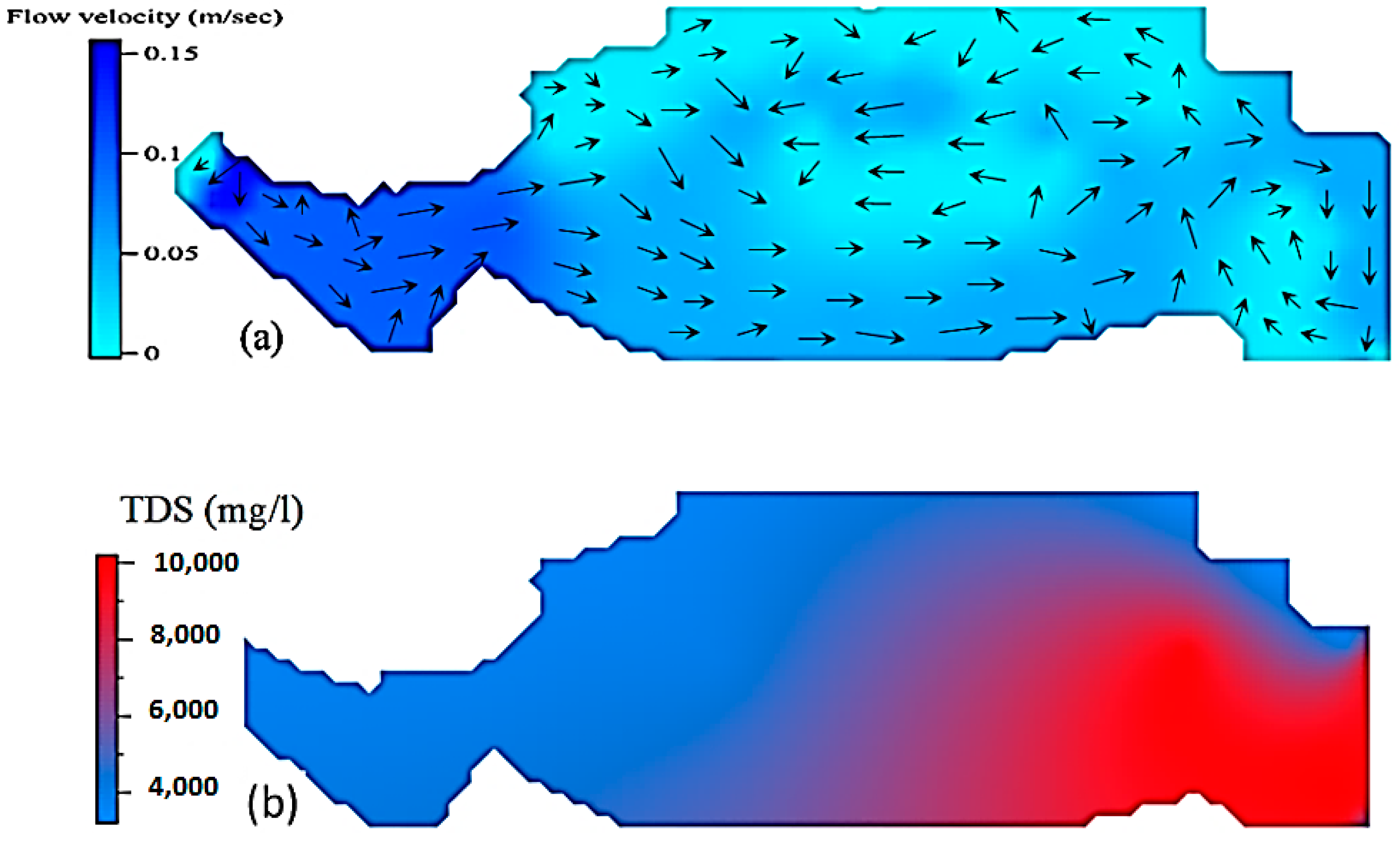
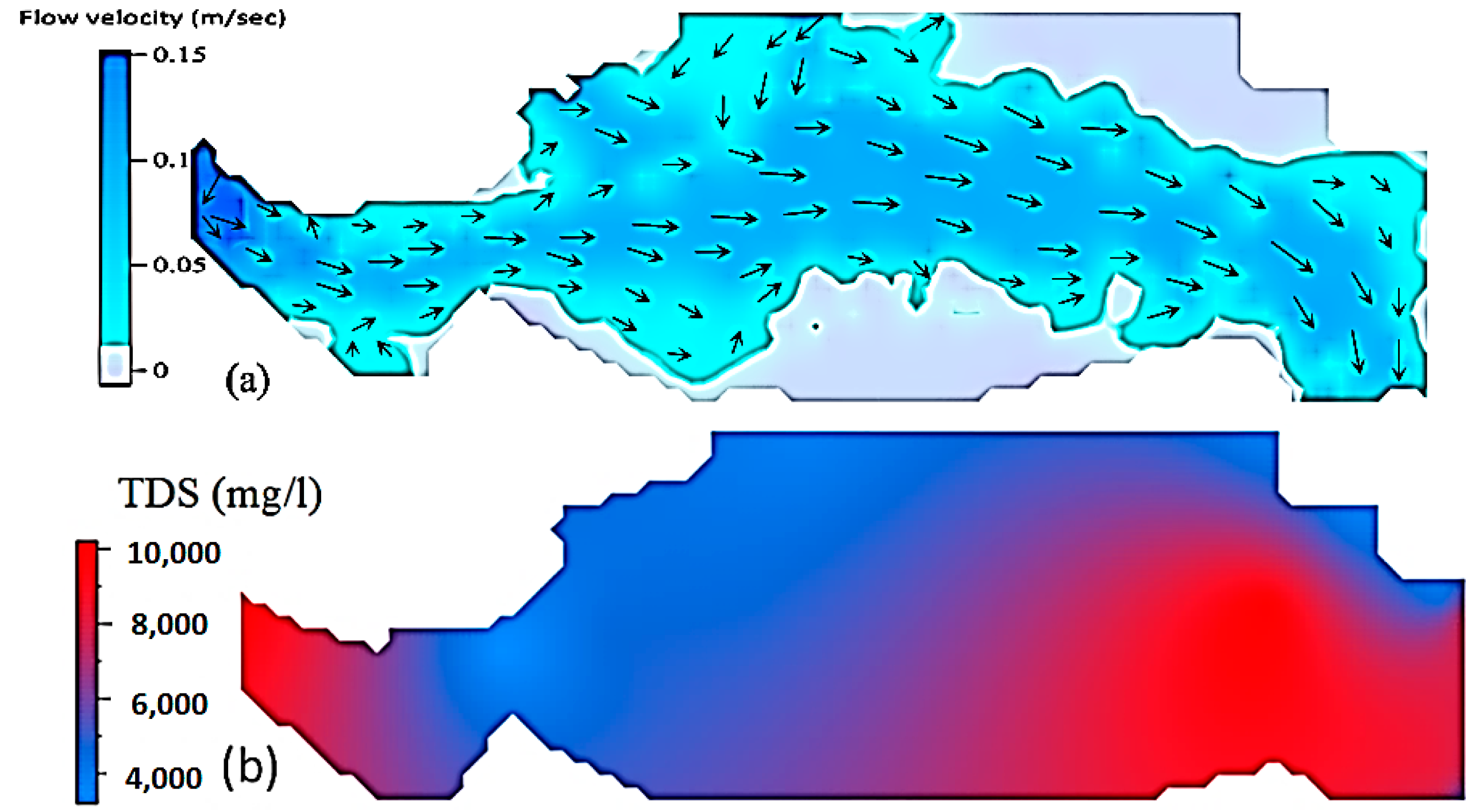
The RMA2 and RMA4 models were consecutively applied for the potential cases of marsh boundary conditions, which are the 30 cases listed in Table 2. Samples of the results of the RMA2 and RMA4 models are shown in Figure 5, Figure 6 and Figure 7 (other are shown in the Supplementary Materials). These figures show the patterns of flow velocity and TDS distribution within the marsh for cases 1, 15, and 30, which can be considered the cases of maximum, average, and minimum inflow, respectively.

The results of the RMA4 models (for the considered WQ parameters) of the 30 considered cases were analyzed using the spatial and temporal analysis tools of GIS. The approach of time-based representations for spatiotemporal data [46] was applied to obtain the time interval of occurrence of a considerable level of change in the concentration of WQ parameters (MA of ±5%) at all the studied MSs (46 MSs). Accordingly, the minimum, average, and maximum SFs (time intervals) of the considered WQ parameters were determined for all the considered 46 MSs (Figure 8). Hence, the SFs of other cases ranged between the SFs of these cases. However, the results of the spatiotemporal analyses show that the minimum SF interval is 11 days. This SF was estimated at 26% of the MSs, MS numbers 15, 16, 17, 19, 20, 21, 22, 23, 29, 30, 31, and 36. These MSs were located within the central and outlet zone of the marsh, except for MS number 36, which was located in the narrow part of the western zone of the marsh. Furthermore, 52% of the MSs had an SF equal to or greater than 14 days. Additionally, a maximum interval of SF of 32 days was estimated at 17% of the MSs, MS numbers 18, 19, 20, 21, 22, 23, 27, and 28. The change in SF from minimum to maximum time interval was based on the considered case of boundary conditions.

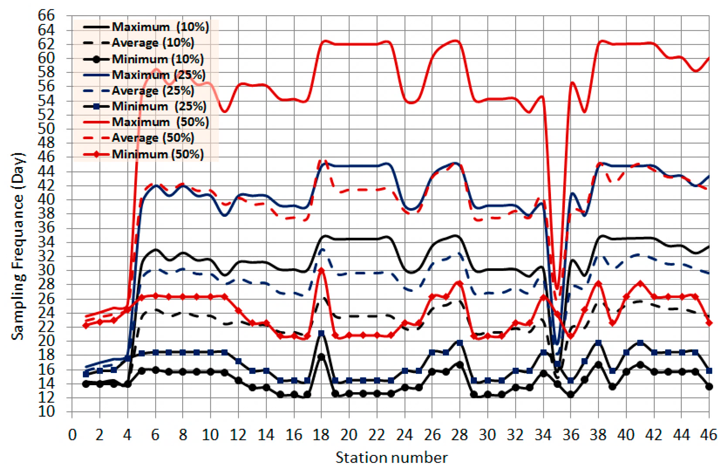
To evaluate the effect of changing the MA, the results of the RMA4 models (WQ parameter distribution patterns) were reanalyzed using the spatiotemporal analysis approach and increasing MA from ±5% to ±50% (stepwise 5%). Figure 9 shows the minimum, average, and maximum interval of SF of the 46 MSs for all the considered WQ parameters with MA of 10%, 25%, and 50%. In addition, the relationship of SF versus the error range (MA) was obtained, see Figure 10. This relationship shows that increasing the MA to ±10%, ±25%, and ±50% increases the minimum (maximum) SF for some MSs by approximately 0% (15%), 7% (40%), and 25% (94%), respectively. With an MA of ±10%, 26% of the MSs had a minimum interval of SF of 13 days, whereas the maximum interval of SF was 35 days, which was estimated at 28% of the MSs. However, with an MA of ±25%, the minimum SF of 4% of the MSs increased one day (to be 14 day) while the minimum SF of remaining percentage of MSs (96%) increased two to five days (to be 15–18 days). However, the maximum interval of SF was 50 days, which was estimated at 28% of the MSs. Moreover, for an MA of ±50%, the minimum and maximum SF increased to 20 and 62 days, respectively.

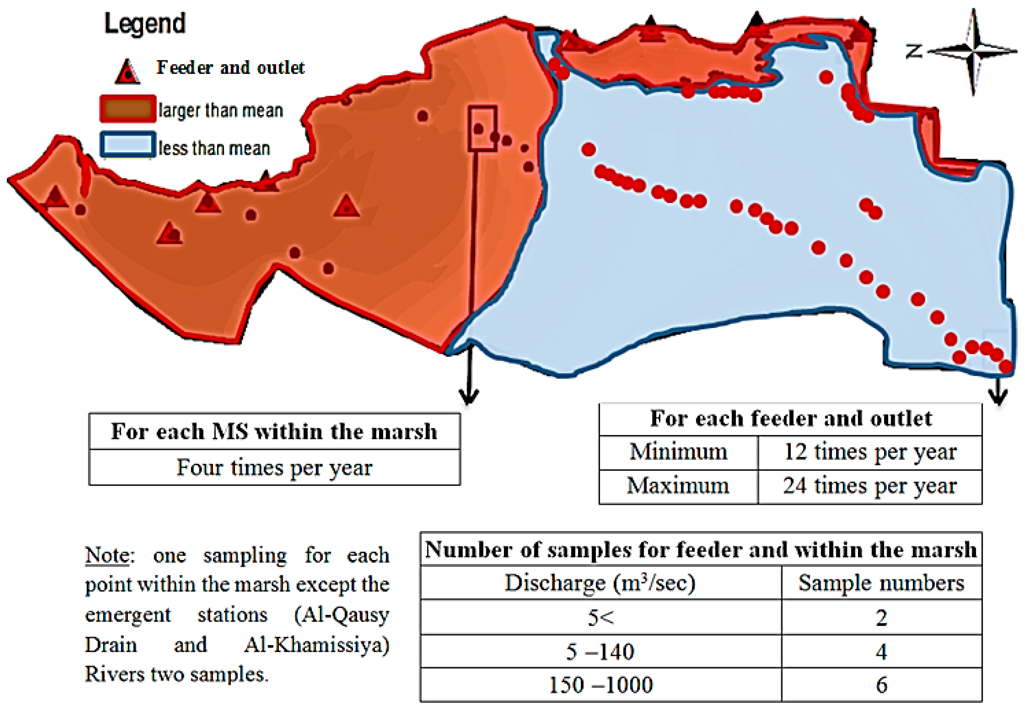
Comparatively, a sampling schedule (Figure 11) was implemented based on the criteria of the sampling frequency for GEMS/WATER stations shown in Table 1 [23]. This time schedule specifies the number of samples and SF for the marsh. According to this schedule, one sample should be taken seasonally from each location within the marsh, whereas for the feeders and outlet, this number depends on the discharge, and each should be taken at least two times per month.

The application of these general guidelines and criteria presents a very permissive schedule of SF, which is four times per year. The proposed methodology specified a minimum and maximum SF interval for each MS that ranged between 33 and 12 times per year (11 and 32 days), respectively. This difference is because applying the general guidelines and criteria does not consider the difference in the sensitivity of pollution detection of the MSs, status of changes of the boundary conditions, complexity of the feeding and drainage system, or analysis of the contaminant distribution patterns. Hence, this traditional design approach does not ensure sufficient detection of all potential pollution waves.

However, the proposed methodology included all the potential values and cases of boundary conditions, which increased the certainty of monitoring the system and the efficiency of the SF schedule. The possibility of occurrence of a case outside of the extreme limits of the boundary conditions is very unlikely. Even if such a case occurs, there is still a high probability that the SF schedule ensures the detection of the changes in pollution level and monitors the flow of pollution surges. This is because the proposed methodology depends on the analysis of the contaminant distribution patterns and the transport velocity of the pollution surges through highly sensitive MSs for the changes in boundary conditions. Additionally, the pollution levels within the water body are highly expected to be within the recorded pollution levels. Even if there is a difference, the transport velocity of the pollution surge between the MSs and the duration of change in pollution level at each MS will not differ much from the specified range using this proposed methodology. Moreover, the hydrodynamic (advection) flow has a greater effect on contaminant transport than that of the diffusion. Therefore, the change in contaminant concentration and location of pollution source within the considered body of water and range of hydraulic changes would not have a large effect on the velocity of the pollution surges, especially considering that the MSs were allocated at the most sensitive locations.

4. Conclusions

Exacerbation of the water scarcity problem in conjunction with the increase in water pollution sources necessitates the development of methods and techniques for water quality monitoring. However, most of the applied design methods are statistical methods and general criteria. These methods are based on a measured dataset collected from nonoptimal preallocated monitoring stations (MS). Therefore, insufficient monitoring is obtained because some effective events or values may not be detected. In this paper, a novel deterministic methodology for estimating the optimal SF for WQMSs has been developed. To this end, contaminant transport simulation models and the GIS tools of spatiotemporal analysis were employed to ensure the detection of a specific level of change in contaminant concentration, taking into consideration all the potential changes in the boundary conditions of a water body. The simulation models and GIS tools were applied to the potential cases of the boundary conditions of Al-Hammar Marsh to determine the minimum SF of the previously allocated 46 MSs with MA values range from the standard level to ±50% (stepwise 5%). Subsequently, the obtained SF schedule using the proposed methodology was compared with those obtained by applying the criteria of GEMS/WATER stations [23]. From the analysis of the results, it can be concluded that the changes in contaminant transport patterns within a water body essentially depend on the cases and values of the boundary conditions. Therefore, the accuracy of monitoring stations at the feeders and outlets of a water body plays a vital role in the accuracy of the obtained SF using any method of determining the SF. Additionally, the geometrical features of a water body or its zones highly affect the velocity and direction of the contaminant distribution within the zones of the water body between the monitoring stations. Consequently, the response of the change in contaminant distribution to the change in boundary conditions differs among the zones of the water body, which affects the determined SF. The SF is highly affected by the values of MA. However, in the considered study area (the western part of the Al-Hammar Marsh), an exponential relationship between SF and MA was obtained. This relationship shows that increasing the MA to ±10%, ±25%, and ±50% increases the SF by approximately 14%, 28%, and 93%, respectively. Hence, the proposed methodology can be used to compute the SF needed to detect a contaminant between MSs within a specific level of MA and vice versa. Utilizing the general criteria and guidelines may give a very permissive schedule of SF. However, in the western part of the Al-Hammar Marsh, applying the general guidelines and criteria gives an SF of four times per year. In contrast, the proposed methodology specifies a maximum and minimum interval of SF for each MS that ranged between 33 and 12 times per year, respectively. The proposed methodology was based on considering all the potential types and values of boundary conditions of the water body. This increases the certainty of the obtained SF and the efficiency of the monitoring system beyond those obtained using other methods. Moreover, the proposed methodology can be applied to all types of surface water resources and can consider any number of MSs with any accuracy level of detectable change. In addition, the proposed methodology provides a detailed database for the distribution patterns of the considered contaminant with the corresponding case and values of boundary conditions.

References

- Bu, H.; Tan, X.; Li, S.; Zhang, Q. Temporal and spatial variations of water quality in the Jinshui River of the South Qinling Mts. Ecotoxicol. Environ. Saf. 2010, 73, 907–913. [Google Scholar] [CrossRef]
- Behmel, S.; Damour, M.; Ludwig, R.; Rodriguez, M.J. Water quality monitoring strategies—A review and future perspectives. Sci. Total Environ. 2016, 571, 1312–1329. [Google Scholar] [CrossRef]
- Thomas, G.S.; Adrian, D.D. Sampling frequency for river quality monitoring. Water Resour. Res. 1978, 14, 569–576. [Google Scholar]
- Loftis, J.C.; Ward, R.C. Water quality monitoring—Some practical sampling frequency considerations. Environ. Manag. 1980, 4, 521–526. [Google Scholar] [CrossRef]
- Robert, H.H.; Michael, J.B. Sampling Frequency for Water Quality Monitoring; Advanced Monitoring Systems Division, Environmental Monitoring Systems Laboratory: Las Vegas, NV, USA, 1981.
- Skalski, J.R.; Mackenzie, D.H. A design for aquatic monitoring programs. J. Environ. Manage. 1982, 14, 237–251. [Google Scholar]
- Don, C.; Peter, N.N.; Dean, H.U. Sampling frequency for water quality monitoring: Measures of effectiveness. Water Resour. Res. 1983, 19, 1107–1110. [Google Scholar] [CrossRef]
- Groot, S.; Schilperoort, T. Optimization of water quality monitoring networks. Water Sci. Technol. 1984, 16, 275–287. [Google Scholar] [CrossRef]
- Steven, P.M.; Dennis, P.L. Optimal design of biological sampling programs using the analysis of variance. Estuar. Coast. Shelf Sci. 1986, 22, 637–656. [Google Scholar] [CrossRef]
- Smith, D.G.; McBride, G.B. New Zealand’s National Water Quality Monitoring Network—Design and First Year’s Operation. Water Resour. Bull. 1990, 26, 767–775. [Google Scholar] [CrossRef]
- Loftis, J.C.; McBride, G.B.; Ellis, J.C. Considerations of scale in water quality monitoring and data analysis. Water Resour. Bull. 1991, 27, 255–264. [Google Scholar] [CrossRef]
- Esterby, S.R.; El-Shaarawi, A.H.; Block, H.O. Detection of water quality changes along a river system. Environ. Monit. Assess. 1992, 23, 219–242. [Google Scholar] [CrossRef]
- Zhou, Y. Sampling frequency for monitoring the actual state of groundwater systems. J. Hydrol. 1996, 180, 301–318. [Google Scholar] [CrossRef]
- Dixon, W.; Chiswell, B. Review of aquatic monitoring program design. Water Res. 1996, 30, 1935–1948. [Google Scholar] [CrossRef]
- Charles, G.H. Relationships between total phosphorus concentrations, sampling frequency, and wind velocity in a shallow, Polymictic Lake. Lake Reserv. Manag. 1999, 15, 39–46. [Google Scholar] [CrossRef]
- Ning, S.K.; Chang, N.B. Multi-objective, decision-based assessment of a water quality monitoring network in a river system. J. Environ. Monit. 2002, 4, 121–126. [Google Scholar] [CrossRef]
- Su-Young, P.; Jung, H.C.; Sookyun, W.; Seok, S.P. Design of a water quality monitoring network in a large river system using the genetic algorithm. Ecol. Model. 2006, 199, 289–297. [Google Scholar] [CrossRef]
- Loftis, J.C.; Ward, R.C. Sampling frequency selection for regulatory water quality monitoring. J. Am. Water Resour. Assoc. 2007, 16, 501–507. [Google Scholar] [CrossRef]
- Harmancioglu, N.B.; Alpaslan, N. Water quality monitoring network design: A problem of multiobjective decision making. Water Resour. Bull. 1992, 28, 179–192. [Google Scholar] [CrossRef]
- Hudak, P.F.; Loaiciga, H.A.; Marino, M.A. Regional-scale ground water quality monitoring via integer programming. J. Hydrol. 1995, 164, 153–170. [Google Scholar] [CrossRef]
- Cieniawski, S.E.; Eheart, J.W.; Ranjithan, S. Using genetic algorithms to solve a multiobjective groundwater monitoring problem. Water Resour. Res. 1995, 31, 399–410. [Google Scholar] [CrossRef]
- Strobl, R.O.; Robillard, P.D. Network design for water quality monitoring of surface freshwaters: A review. J. Environ. Manag. 2008, 87, 639–648. [Google Scholar] [CrossRef] [PubMed]
- UNEP/WHO. Water Quality Monitoring—A Practical Guide to the Design and Implementation of Freshwater Quality Studies and Monitoring Programmes; Bartram, J., Balance, R., Eds.; United Nations Environment Programme (UNEP)/The World Health Organization (WHO): Nairobi, Kenya; Geneva, Switzerland, 1996; ISBN 0 419 22320 7 (Hbk); 0 419 21730 4 (Pbk). [Google Scholar]
- Timmerman, J.G.; Adriaanse, M.; Breukel, R.M.A.; Van Oirschot, M.C.M.; Ottens, J.J. Guidelines for water quality monitoring and assessment of transboundary rivers. Eur. Water Pollut. Control 1997, 7, 21–30. [Google Scholar]
- Dixon, W.; Smyth, G.K.; Chiswell, B. Optimized selection of river sampling sites. Water Res. 1999, 33, 971–978. [Google Scholar] [CrossRef]
- Khalil, B.; Ouarda, T.B. Statistical approaches used to assess and redesign surface water-quality-monitoring networks. J. Environ. Monit. 2009, 11, 1915–1929. [Google Scholar] [CrossRef]
- World Meteorological Organization. Planning of Water Quality Monitoring System; Technical Report; Series No. 3; World Meteorological Organization: Geneva, Switzerland, 2013; ISBN 978-92-63-11113-5. [Google Scholar]
- Kaya, I.; Kahraman, C. Multicriteria decision making in energy planning using a modified fuzzy TOPSIS methodology. Expert Syst. Appl. 2011, 38, 6577–6585. [Google Scholar] [CrossRef]
- Huu, T.D.; Shang-Lien, L.; Lan Anh, P.T. Calculating of river water quality sampling frequency by the analytic hierarchy process (AHP). Environ. Monit. Assess. 2013, 185, 909–916. [Google Scholar] [CrossRef]
- Holnicki, P.; Nahorski, Z.; Żochowski, A. Modelling of Environment Processes; Wydawnictwo Wyższej Szkoły Informatyki Stosowanej i Zarządzania: Warszawa, Poland, 2000. [Google Scholar]
- Balcerzak, W. Application of selected mathematical models to evaluate changes in water quality. In Proceedings of the International Conference on Water Supply, Water Quality and Protection, Kraków, Poland, 7–9 September 2000. [Google Scholar]
- Al-Khafaji, M.S.; Abdulraheem, Z.A. A deterministic algorithm for determination of optimal water quality monitoring stations. Water Resour. Manag. 2017, 31, 3575–3592. [Google Scholar] [CrossRef]
- WMO (World Metrological Organization). Guide to Hydrological Practice, 6th ed.; No. 168; World Metrological Organization: Geneva, Switzerland, 2008; Volume I. [Google Scholar]
- Alhamdani, J.S. Location of Outlet and Operation of the West Part of Al-Hammar Marsh. Ph.D. Thesis, University of Baghdad, Baghdad, Iraq, 2014. [Google Scholar]
- Iraqi Ministry of Environment. New Eden Master Plan for the Integrated Water Resources Management in the Marshland Area, Marshlands, Book 4; Iraqi Ministries of Environment, Water Resources Municipalities and Public Works with cooperation of the Italian Ministry for the Environment and Territory and Free Iraq Foundation: Baghdad, Iraq, 2006; p. 130. [Google Scholar]
- Al-Gburi, H.F.; Al-Tawash, B.S.; Al-Lafta, H.S. Environmental assessment of Al-Hammar Marsh, Southern Iraq. Heliyon 2017, 3, e00256. [Google Scholar] [CrossRef] [Green Version]
- Al-Musawi, N.O.; Al-Obaidi, S.K.; Al-Rubaie, F.M. Evaluating Water Quality Index of Al Hammar Marsh, South of Iraq with the Application of GIS Technique. J. Eng. Sci. Technol. 2018, 13, 4118–4130. [Google Scholar]
- APHA. Standard Methods, The Examination of Water and Wastewater, 22nd ed.; APHY: Washington, DC, USA, 2012; p. 1496. [Google Scholar]
- Young, J.C.; Mcdermott, G.N.; Jenkins, D. Alterations in the bod procedure for the 15th edition of standard methods for the examination of water and wastewater. J. Water Pollut. Control Fed. 1981, 53, 1253–1259. [Google Scholar]
- Harris, D.C. Quantitative Chemical Analysis, 4th ed.; W.H Freeman and Company: New York, NY, USA, 1995; Chapter 21. [Google Scholar]
- Raghavan, R.; Raha, S. A rapid turbidimetric method for the determination of total Sulphur in zinc concentrate. Talanta 1991, 38, 525–528. [Google Scholar] [CrossRef]
- Armstrong, F.A.J. Determination of nitrate in water by ultraviolet spectrophotometry. Anal. Chem. 1963, 35, 1292–1294. [Google Scholar] [CrossRef]
- Soltani, F.; Kerachian, R.; Shirangi, E. Developing operating rules for reservoirs considering the water quality issues: Application of ANFIS-based surrogate models. Expert Syst. Appl. 2010, 37, 6639–6645. [Google Scholar] [CrossRef]
- Donnell, B.P.; Letter, J.V.; McAnally, W.H. User Guide to WES-RMA2 Version 4.5; Waterways Experiment Station, Costal and Hydraulics Laboratory: Davis, CA, USA, 2004. [Google Scholar]
- Peuquet, D.J.; Duan, N. An event-based spatio-temporal data model (ESTDM) for temporal analysis of geographic data. Int. J. Geogr. Inf. Syst. 1995, 9, 2–24. [Google Scholar] [CrossRef]
- Peuquet, D.J.; Wentz, E. An approach for time-based analysis of spatio-temporal data. In Proceedings of the Sixth International Symposium on Spatial Data Handling, Edinburgh, UK, 5–9 September 1994; International Geographical Union: London, UK, 1994; pp. 489–504. [Google Scholar]
Figure 1.
Layout of the Al-Hammar Marsh.
Figure 2.
Topography of the Al-Hammar Marsh.
Figure 3.
Manning’s roughness coefficients of the Al-Hammar Marsh [34].
Figure 4.
Locations of the measurement positions.
Figure 5.
Distribution patterns of the flow velocity and TDS for the maximum inflow (Case 1). (a) Velocity pattern. (b) TDS pattern.
Figure 6.
Distribution patterns of the flow velocity and TDS for the average inflow (Case 15). (a) Velocity pattern. (b) TDS pattern.
Figure 7.
Distribution patterns of the flow velocity and TDS for the minimum inflow (Case 30). (a) Velocity pattern. (b) TDS pattern.
Figure 8.
Minimum, average, and maximum interval of SF of the 46 MSs, with MA of ±5%.
Figure 9.
Minimum, average and maximum interval of sampling frequency (SF) of the 46 monitoring stations (MSs), with monitoring accuracies (MA) of ±10%, ±25%, and ±50%.
Figure 10.
Relationship of SF versus MA.
Figure 11.
Sampling schedule using [23].