Relative Effect of Location Alternatives on Urban Hydrology. The Case of Greater Port-Harcourt Watershed, Niger Delta

Institute of Geography, The University of Edinburgh, Edinburgh EH8 9XP, UK
*
Author to whom correspondence should be addressed.
Hydrology 2019, 6(3), 82; https://doi.org/10.3390/hydrology6030082
Submission received: 20 September 2018
/
Revised: 11 August 2019
/
Accepted: 23 August 2019
/
Published: 17 September 2019
(This article belongs to the Special Issue Advances in Integrated Watershed Modeling: Emerging Water Issues under Changing Land Use and Climate)
Abstract
:Globally, cities in developing countries are urbanising at alarming rates, and a major concern to hydrologists and planners are the options that affect the hydrologic functioning of watersheds. Environmental impact assessment (EIA) has been recognised as a key sustainable development tool for mitigating the adverse impacts of planned developments, however, research has shown that planned developments can affect people and the environment significantly due to urban flooding that arises from increased paved surfaces. Flooding is a major sustainable development issue, which often result from increased paved surfaces and decreased interception losses due to urbanisation and deforestation respectively. To date, several environmental assessment studies have advanced the concept of alternatives, yet, only a small number of hydrologic studies have discussed how the location of paved surface could influence catchment runoff. Specifically, research exploring the effects of location alternative in EIAs on urban hydrology is very rare. The Greater Port-Harcourt City (GPH) development established to meet the growth needs in Port-Harcourt city (in the Niger Delta) is a compelling example. The aim of this research is to examine the relative effect of EIA alternatives in three different locations on urban hydrology. The Hydrologic Engineering Centre’s hydrologic modelling system (HEC-HMS) hydrodynamic model was used to generate data for comparing runoff in three different basins. HEC-HMS software combine models that estimate: Loss, transformation, base flow and channel routing. Results reveal that developments with the same spatial extent had different effects on the hydrology of the basins and sub-basins in the area. Findings in this study suggest that basin size rather than location of the paved surface was the main factor influencing the hydrology of the watershed.
1. Introduction
Flooding remains the most re-occurring natural disaster in recent decades [1]. The relationship between flooding and urban growth in coastal cities have been investigated in a plethora of studies [2,3,4,5,6]. A number of these studies have suggested that understanding the anthropogenic factors and options that compound flood risk should remain a priority [2,7]. A complex blend of factors, including climate change, land use changes, high tide, low topography, poorly implemented regulations, lack of integrated planning, etc. have often resulted in environmental degradation and disproportionate impacts of natural disasters affecting millions worldwide [2,7]. Apart from flood impact, research have also reported that urbanisation can have detrimental effects on water quality and soils. Increased urban land cover alter water quality in terms of nutrients (N, P and C), dissolved oxygen (DO) and suspended sediment [8,9], on the other hand the stream bed undergoes recurrent erosion due to higher and more frequent floods resulting from urbanisation [10,11].
Recent studies have reported that countries in Africa and Asia are the most vulnerable to flood disasters. For example, the last decade (2006–2015) witnessed about 1700 flood events globally, but, approximately 76% of these flood events occurred in Africa and Asia. During this period, about 57,000 flood related deaths were reported and around 87% of these deaths occurred in Africa and Asia [12]. Despite the worrying trend, urban flood risk research is lagging way behind in developing countries compared to developed countries.
Urban flooding resulting from extreme runoff has been extensively researched as a planning, watershed and disaster management problem [13,14]. It is a product of the interaction of physical and human-induced factors. Urbanisation, environmental regulations and extreme precipitation are among the human factors that compound flooding. Urbanisation refers to the concentration of the population and a process of change in land-use and conversions. Hence, of all types of land use change, urbanisation is considered the most dramatic in terms of its effects on flooding [6,15,16,17]. The most concern to hydrologist and planners is the alternatives/options that affect the hydrologic functioning of watersheds [15,18,19], yet, to date research assessing the effects of urban land-use alternatives on flooding is rare. It is important to note that alternative/options in this study refer to the alternative locations of urban development in environmental impact statements.
Environmental impact assessment (EIA) is a systematic process of identifying, predicting, evaluating, and mitigating the biophysical, social and other relevant effects of proposed projects and physical activities prior to major decisions and commitments being made [20]. EIA is now globally recognised as a key instrument for managing and regulating planned developments [21,22,23]. Studies show that EIA is now widely adopted in several jurisdictions [24,25,26,27], and the consideration of alternatives is at the heart of the assessment process [20,28]. The consideration of alternatives involves the evaluation of a range of options for meeting the objectives of project plans [24], with a goal to make a rational selection of the ‘best option’.
On the other hand, unplanned or scattered developments often referred to as ‘urban sprawl’ can occur in several forms [25]. From a planning perspective, they are considered undesirable and non-compact archetypes of development [29], which can exist in a form of continuous low-density, leapfrog and ribbon development [25]. Paradoxically, research has also shown that planned like unplanned developments can have significant impacts on people, amenity the environment due to flooding resulting from increased paved (impermeable) surfaces.
Urban flooding, resulting from extreme runoff, has been extensively researched as a planning, watershed and disaster management problem [13,14]. Unlike the location of paved surfaces, factors such as basin size, drainage density and topography are often discussed, but, in hydrology, the location of impermeable surfaces is an important factor and can affect runoff in catchments [30,31,32]. Therefore, the study of location alternatives in environmental impact statements (EIS) for urban planning is significant.
Although studies comparing the effects of impact assessment alternatives on flooding are scanty, some studies have attempted to understand the environmental performance of different land-cover types in an urban system (with different subunits, i.e., housing schemes, commercial and industrial developments and services) on flooding in Munich, Germany [18]. However, the emphasis of that study was not on location or position of the development within the basin. Another study investigated how planning alternatives could affect critical habitats [33]. Again, the aim of the later study was rather to understand the impact on aquatic life.
In terms of EIA alternatives, a good number of studies have advanced the concept of alternatives in EIA literature [28,34,35,36,37,38,39,40]. Key aspects discussed in EIA literature include benefits and types of alternatives in Glasson et al. [28]; the process for developing alternatives in González, Thérivel [31]. An important gap in these studies is a lack of focus the effect of different alternatives on environmental systems such as the hydrologic cycle. To the best of the author’s knowledge, published work on the effects of location alternative on urban hydrology is very rare.
Greater Port-Harcourt (GPH) city in the Niger Delta is a compelling example of rapidly developing cities in a hydrologically sensitive region. To meet the growth need in the city, the GPH city development master plan currently in Phase 1 was established [41,42]. An EIA accompanied Phase 1 project plan of the Master plan, and the current project location in Port-Harcourt was chosen as the preferred site between two other alternative locations in the Bori and Omoku/Ogba areas [38]. Site selection was carried out based on planning and economic considerations such as the availability of land, the commitment of available space to other land-uses, contiguity of open space to the old city and financial cost [42], not considering flood risk implication.
The aim of this research is to understand the relative impact of developments in the alternative locations on the basin and sub-basin hydrology in the GPH watershed. Key questions asked include: Did the developments affect the hydrology of the watershed? Which alternative would be the least disruptive in terms of impact on flooding?
2. Study Area
2.1. Description of Study Area
Greater Port-Harcourt (GPH) is a coastal mega city located in the southeastern flank of the Niger Delta, between latitude 4°45′N and latitude 4°55′N, and longitude 6°55′E and longitude 7°05′E in Rivers State, with an administrative area of about 1900 km2. The Niger Delta is a coastal region with distinctive geography demarcated by a natural delta of the River Niger system located in the Gulf of Guinea [39,40]. The studied watershed (Figure 1a) is flat and consists of a low-lying coastal plain that is barely 20 m above sea level made up of five major basins and 39 sub-basins, covering about 4820 km2. The climate of Port-Harcourt falls under Af, that is an equatorial monsoon climate, according to the Köppen-Geiger climate classification [41]. Rainfall is significant for most months of the rainy season (April to Nov), but short spells of dry season occur (November–March) with little effect. Usually, the mean monthly rainfall is highly varied in the area, with an average of 2400 mm. Rainfall is the major cause of flooding in the area [43,44,45].
Port-Harcourt is the fourth largest city in Nigeria after Lagos, Kano and Ibadan [46]. It is the administrative capital of Rivers State and the largest city in the Niger Delta with a population exceeding two million inhabitants [47]. Administratively, GPH is an agglomeration of eight local communities neighbouring Port-Harcourt city. Prior to the establishment of Greater Port-Harcourt law, Port-Harcourt city consisted of three local governments including Obio-Akpo and Okrika areas. The GPH city now includes Ikwerre, Oyigbo, Ogu-bolo, Etche and Eleme administrative areas, due to the newly established urban Master plan.
Due to the proximity to the coast, the city was established as a rail and seaport terminal for exporting coal and agricultural produce from the northern part of Nigeria [48]. Like other oil cities, the discovery of oil and gas accelerated the industrial and commercial expansion in Port-Harcourt. By 1965, the municipality became the site of Nigeria’s largest harbour and the centre of Nigeria’s petroleum activities [49]. Since then, there has been a constant influx of people into the metropolis. Apart from the rise in population, the city is expanding physically, which is why to date, the city’s planning authority have struggled to cope with the urban growth. In a nutshell, economic activities in the city have led to a high influx of people and overcrowding, resulting in rapid urban expansion [42].
2.2. Description of Project
In response to the overcrowding issues, the Greater Port-Harcourt Development Authority (GPHDA) was established in 2009 to expand the city strategically. Implementation of the Master plan was carried out in Phases 1, 2, and 3 (Figure 1b). Subsequently, the EIA study was carried out to assess the potential and associated impacts of the proposed Phase 1 projects. In 2018, Phase 1 was still at the construction stage of the project cycle and was expected to be completed by 2020.
The Phase 1 layout covers about 1692.07 ha (16.921 km2) extending from the Port-Harcourt International Airport junction across to Professor Tam David-West road to part of the Igwuruta area. The ongoing project layout comprises of clusters of neighbourhoods including low, medium and high-density residential area, mixed-use complexes, schools, churches, golf course and estates.
Project activities covered under Phase 1 include the construction and operation of: A 132 kV double circuit transmission line; a 132/33/11 kV 100 MVA substation; bulk water abstraction, storage and supply system; priority road and internal street network; construction of a sewage treatment plant and its associated reticulated pipeline network; a sanitary engineered landfill waste disposal facility to service the new city and 3000 houses, the housing estate will be accompanied with internal services consisting of: Internal roads; a sewage, drainage and storm water system; a power reticulation system; a solid waste handling facility and a potable water reticulation system [38,49]. The Phase 1 project activities include the construction and operation of the new Rivers State University of Science and Technology (2.12 km2), Sports precinct (0.5 km2) in addition to the 1000-bed mega hospital complex.
Consideration of location alternative was an important part of the project planning process. The current location north of Port-Harcourt city (at the centre of the map in Figure 1a) was the preferred choice. Supplementary locations considered for the project included the Omoku/Ogba area northwest of the old city and the Bori area situated southeast of the old city. The supplementary locations were considered non-contiguous to the old Port-Harcourt city.
According to Verml [42], the supplementary location alternatives are several kilometres away from the old city. From a planning standpoint, these alternative locations were rejected due to the huge financial cost and resources required to construct an entirely new city. However, from a sustainability standpoint Sadler [20] maintains that EIAs should compare location alternatives to determine the most environmentally friendly or best practicable environmental option (BPEO). Glasson, et al. [50] added that the decisions for preferred location alternative should not only be based on the need to maximise economic and planning benefits but also on environmental benefits.
3. Materials and Methods
The procedure for comparing the relative impacts of location alternatives followed four main stages in this study, namely: Data acquisition, preparation of spatial and topographical data, mapping of alternative locations and hydrological modelling and data analysis.
3.1. Data Acquisition
As the basic inputs for hydrological modelling, soil, topographical, spatial and rainfall data were obtained from different sources for the analysis.
Soil, Topographical and Rainfall Data
Soil maps together with land use/land cover (LULC) maps were the primary data used for generating curve numbers (CN). There was no readily available soil map for determining hydrologic soil group (HSG) for the area. Therefore, a 1:1,000,000 digital soil maps were obtained from the United Nation’s Food and Agricultural Organisation (FAO). Soils in the same hydrologic soil group represent soils that have similar runoff potential under similar storm and land-cover conditions. They determine the associated runoff curve number of a soil [51].
The runoff curve number is used to estimate direct runoff from rainfall. To generate soil data, the following procedure was followed. First, 1:1,000,000 digital soil maps were obtained and merged. Then the merged soil map was clipped, and re-classified based on soil texture. Two main types of soils were identified (clay and sandy clay), as such two types of HSGs were categorised in the area (see Table 1). Generally, HSG soil groups are divided into HSG A, B, C and D, as such their runoff potential increases from A to D [52,53].
HSG A soils have an infiltration rate greater than 0.3 in/h and are predominantly sand or gravel soils with low runoff potential. HSG B are soils characterised by infiltration rates ranging from 0.15 to 0.30 in/h and are moderately coarse soils. The infiltration rate of HSG C soils ranges from 0.05 to 0.15 in/h and are moderately fine to fine soils that can impede water flow. For HSG D, the infiltration rate is less than 0.05 in/h and are typically very fine soils (clay soils) with high runoff potential [52]. As shown in Table 1, this study area was mainly covered with HSG C (i.e., sandy clay soils) and HSG D (clay) soils. That is soils characterised by low and very low infiltration rates.
Topographical data is a key input for hydrological modelling. The main way of characterising topography is by the use of satellite-based digital elevation model (DEM), which requires high-accuracy as well as high-resolution elevation data [54,55]. The freely available 90 m × 90 m shuttle radar topography mission (STRM) DEM applied in this study was downloaded from the United States Geological Survey (USGS) website. Two SRTM DEM tiles-38_11 and 38_12 tiles were merged, clipped, masked and used for extracting the channel characteristics and delineating sub-basins. One limitation with this data is its coarseness when compared to the 1-arc DEM available for the North American continent. Hence, the 90 m × 90 m STRM data was acceptable because several published studies have also used it for generating results [56,57]. These studies reveal that large vertical errors in SRTM data are lesser in areas with low- to medium relief [56,57,58]. Therefore, the applied dataset was deemed reliable for modelling the hydrology of this low-lying watershed.
3.2. Acquisition of Land Use Data and Processing
Land use and land cover data also play a crucial role in hydrology research. They are often used to generate landscape-based metrics, monitor status and assess landscape conditions as well as trends over a specified time interval [59,60,61]. The 30 m ETM+ Landsat imagery (Figure 1a) for year 2003 was obtained from the USGS earth explorer website and the main reason for using ETM+ sensor data was, firstly, due to availability. Secondly, it provides data covering the spatial extent of the entire study area. Although the higher resolution light detection and ranging (LiDAR) data can provide a more accurate estimate [62,63], it was not available for the study area at the time of this research. The 1:1,100,000 scale LULC map had cloud cover under 20%. Classification of the Landsat imagery was performed using the maximum likelihood classification. The procedure followed involves geometric rectification, image enhancement and maximum likelihood classification.
3.3. Mapping the Alternative Locations
Mapping and estimation of future LULC changes followed five main stages including: Selection of location alternatives for mapping, digitisation of hard copy GPH maps, interpretation/reclassification of GPH LULC maps, overlay of digital maps on baseline map and the estimation of future LULC changes. The goal was to compare the relative effects of the location alternative on peak discharge at basin and sub-basin scale. However, two assumptions were made prior to mapping the alternative. First, due to data limitation, the 2003 LULC map represented the baseline condition. Second, the 2060 urban LULC condition was mapped assuming that the conditions of other LULC classes outside the GPH map would largely stay the same.
Three locations were selected namely, Bori, Ogba/Omoku and Port-Harcourt (the current project) alternative. Next, digitisation was performed by converting the geographic features of the Phase 1 analogue map into a digital format. Digitisation process was done, first by georeferencing the analogue maps (Master plan and location alternative maps) to an appropriate projected coordinate system i.e., WGS_84_UTM_zone_32N. Second, by creating an empty shape file. Third, by digitising the LULC classes. The GPH Masterplan was reclassified into four main classes i.e., urban, forest, agriculture and mangrove. To map location alternatives to the current project, the Phase 1 feature was then dragged to the three locations (at Bori, Ogba/Omoku and Port-Harcourt) as specified in the EIS report.
3.4. Hydrologic Modelling
3.4.1. The Hydrological Model
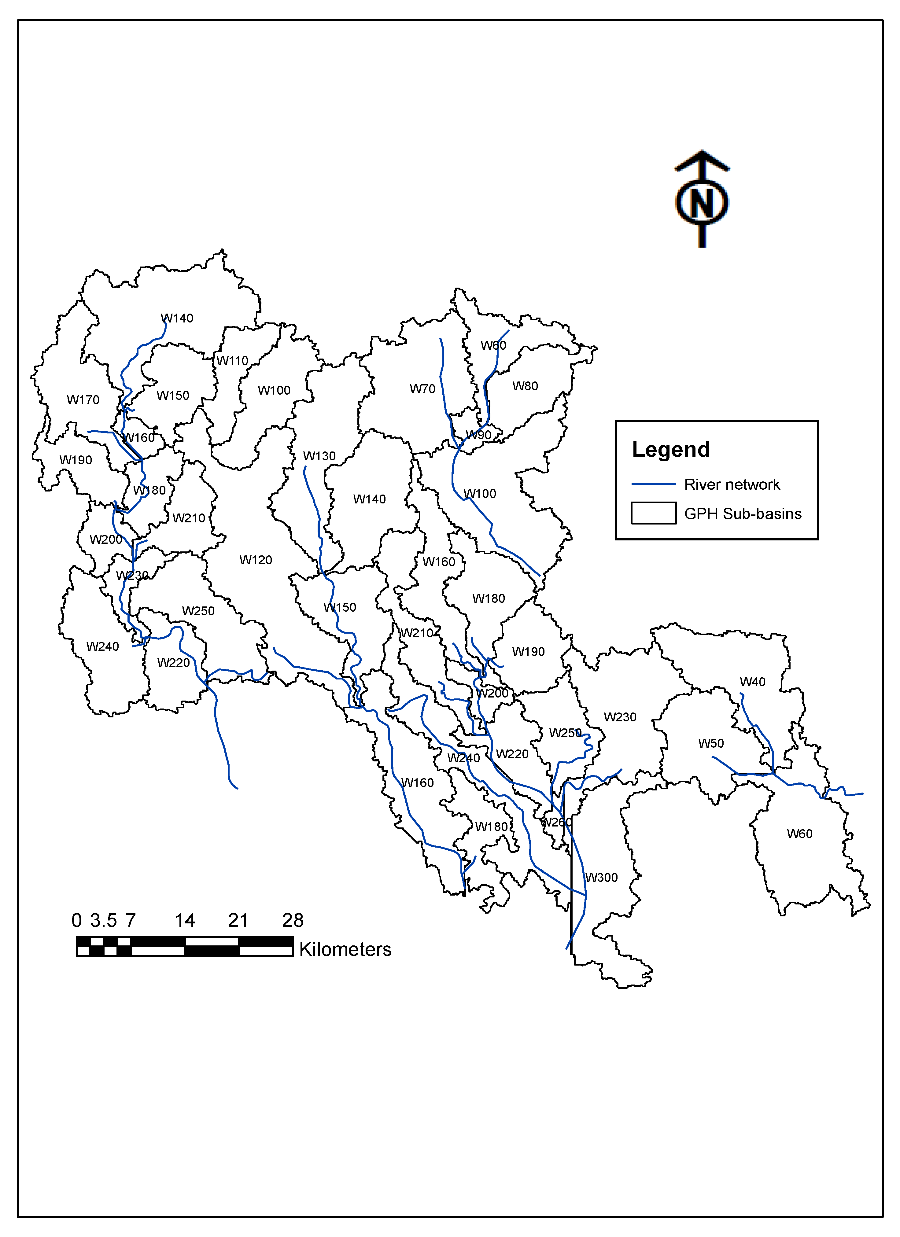
The rainfall-runoff modelling was performed using the Hydrologic Engineering Centre’s hydrologic modelling system (HEC-HMS). HEC-HMS and HEC-GeoHMS in ArcMap used for simulation were developed by the US Army Corp of Engineers (USACE) [52]. The model was used for simulating rainfall-runoff and routing process of the dendritic watershed. Modelling was performed for four basins and 34 sub-basins (Figure 2) and the purpose was to compare the effects of the three alternative locations on peak discharge.
HEC-HMS uses separate sub-models to represent each component of the runoff process. The HEC-HMS software combines models that estimate: Loss (runoff volume), transformation (discharge runoff), base flow and channel routing respectively [52,64,65]. In each model run, the basin model, the precipitation model and the control model were coupled to generate results. The basin model consists of the basin elements, connectivity data and routing parameters and these were used to model the physical processes in the watershed. The precipitation model contained the meteorological data for the model, while the control model was used to manage the time series data in the model.
3.4.2. Model Pre-Processing
Prior to model application, a series of pre-processing tasks were performed with the input data using HEC-GeoHMS and Arc-Hydro tools in ArcGIS. HEC-GeoHMS is the Hydrologic Engineering Centre’s geospatial modelling extension. Model pre-processing mainly involved terrain processing, watershed processing, basin processing and basin extraction.
3.5. Model Set Up
3.5.1. Loss Model
The Basin model was used to represent and construct the physical characteristics of the watershed under study. In this study, the Soil Conservation Service (SCS)-curve number (CN) loss model was used to simulate runoff volume or precipitation excess as a function of cumulative precipitation, land-use, soil cover and antecedent moisture conditions [4,52,66]. There are a variety of loss models, but the empirical SCS-CN method was adopted for computing infiltration loss in this study. This was because it relied on just one parameter and is less data intensive. The underlying theory is that runoff can be related to soil-cover complexes and rainfall through a curve number.
The SCS CN was estimated using the following empirical relationships
The maximum retention (S) was calculated with the equation:
Substituting Equation (3) into Equation (4) and this gives:
where Q = runoff; P = accumulated rainfall depth at time t; Ia = the initial abstraction (or initial loss) and S = potential maximum retention. Note: CN (curve number) is an index that characterises the combination of the land-use classes, the hydrologic soil group (HSG) and antecedent moisture content (AMC) [4,52].
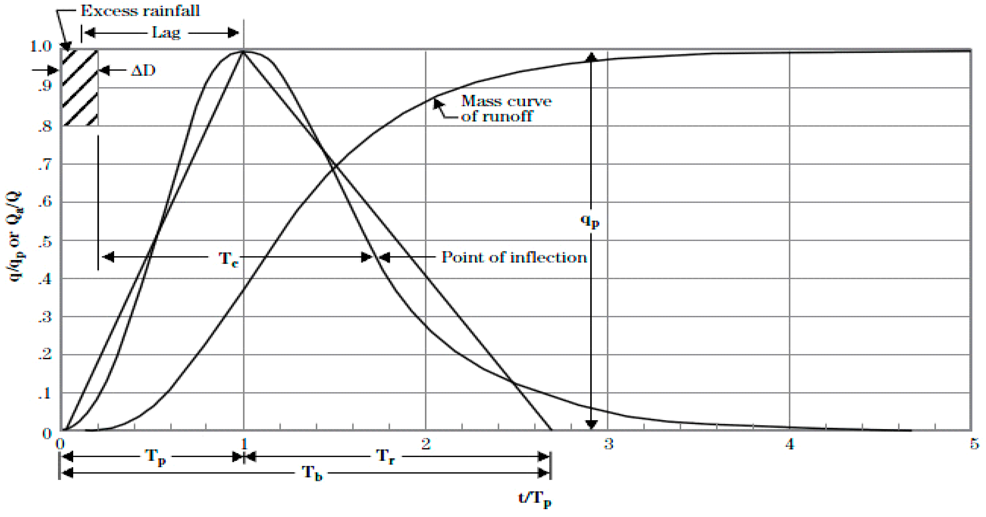
For modelling runoff transformation, the SCS dimensionless unit hydrograph (DUH) was the empirical model applied. The model was based on the unit hydrograph theory. The SCS UH model is a dimensionless single-peaked DUH and expresses the DUH discharge as the ratio to peak discharge (Qp), for any given time t, a fraction of the time of the DUH peak (Tp). By using the SCS DUH, the objective was to determine three variables namely lag time L (h), time to peak, Tp (h), and peak discharge, Qp (m3/s).
3.5.2. Runoff Model
For runoff transformation, the SCS dimensionless unit hydrograph (DUH), an empirical model based on the unit hydrograph theory was applied. Figure 3 presents a diagram of the unit discharge hydrograph resulting from one inch of direct runoff, distributed uniformly over the watershed resulting from rainfall of a specified duration. The SCS DUH model is a dimensionless single-peaked unit hydrography and expresses the hydrograph discharge as the ratio to peak discharge (qp), for any given time t, and for a fraction of time of peak (Tp). SCS DUH was determined using three main parameters: Lag time, L (h), time to peak, Tp (h), and peak discharge, qp (m3/s), see equations 5 to 8. Importantly, assumptions of linearity and time-invariance were made as stated in Feldman [52].
The Natural Resources Conservation Service (NRCS) proposes that UH peak (qP) and time of UH peak (TP) are related by:
where,
- A = the drainage area,
- Q = the runoff volume (excess rainfall; derived from Eq. 4.7),
- TP = the time to peak in hours,
- qP = the peak flow.
Time to peak or time of rise equals to the duration of the unit excess precipitation ∆t given by the following equation
where = excess precipitation duration (which is the computational interval in HMS).
The basin lag (Tlag) is defined as the time difference between peak rainfalls and peak discharge
Note: Lag time was the only parameter automatically calculated in the model.
Basin lag time was solved by:
In this project, lag parameter values were derived from Tc computed and was calculated automatically using the values of slope and maximum flow lengths derived from the DEM. Lag parameter was imported into the basin model and was then computed for all sub-basins. The SCS DUH was used because the minimum input data required for estimating the peak discharge in ungauged watersheds [52,66]
3.5.3. Routing
For routing flow along river reaches, the Muskingum–Cunge method was applied. Unlike the Muskingum method, the Muskingum–Cunge model uses the relationship between channel properties and parameters [67]. Channel geometry information such as channel slope, length, shape, bottom width and side slope were derived from the DEM. This is a reliable alternative for determining parameters X and K and for simulating open channel discharge downstream in ungagged river channels. K equals the flood wave time travel through the reach and X equals the dimensionless weight () [68].
3.6. Model Application
After the terrain processing, and parameter estimation, the HEC-HMS 4.0 software was utilised for computing. In each model run, the basin model, precipitation model and the control model were coupled for generating results following procedures in USACE [67].
3.6.1. Basin Model
The basin model consists of the basin elements, connectivity data and routing parameters and these were used to model the physical processes in the watershed.
First, the basin model was used to represent and construct the physical characteristics of the watershed. Hydrologic elements such as sub-basins, reaches, outlets and junctions were added from HEC-GeoHMS and connected to model the real world. Note, the imported files contained estimated parameters such as curve number (CN) and percentage of impermeable surface (PctImp), basin attributes and elevation data was managed in the basin model component.
3.6.2. Precipitation Model
The precipitation model component was used to model rainfall. In this study, the hyetograph method was applied. The total depth option was used for running the future event, and the statistically derived rainfall depth of 290.09 mm was inputted for the 100-year design storm.
3.6.3. Control Model
The control specification component was used for regulating timing and was comprised of duration, start and end times as well as the time step for the simulation. The duration of the projected storm was 24 h and a 10 min time step was applied for all model runs.
3.7. Model Calibration
Calibration of the model for this study was challenging due to the unavailability of observed discharge data and this is a typical problem for hydrology research in most developing regions. To overcome this problem, an alternative method-prediction in the ungagged basin (PUB) approach was adopted as described by Roy [68] and Ford [66]. In this method, the model parameters for loss, transform and channel routing were mainly derived from the digital elevation model (DEM), soil and satellite land cover maps. The PUB approach uses the characteristic of the watershed. These are the physical, measurable properties of the watershed such as area, slope, roughness coefficient, channel slope, channel bottom width, reach length, etc. [66,69].
Loss-initial abstraction parameters were estimated in HEC-HMS using the CN values. Transform-lag parameters were also estimated using longest flow path and distance to basin centroid derived from the DEM. Flow in river channels were modelled using the Muskingum–Cunge method with inputs such as channel length, slope, channel shape, side slope, and channel width as well as roughness coefficient (Manning’s n), Table 2.
3.8. Model Validation
Model validation is the final and important level of any model analysis that deals with uncertainty and accuracy. In this study, validation of the HEC-HMS model was performed for four-year time periods: 1985, 1987, 1988 and 1989 respectively. These time periods selected for validation were different from those used in the model run and are based on time periods for which observed peak discharge data were available. Observed peak discharge data for a nearby River Basin (Imo River Basin) was obtained from recent published work by Okoro and Uzoukwu [70] spanning 1985 to 1998. The data was useful for validating the model estimates in the absence of adequate data. In this study, it was assumed that good model performance for the Imo River basin would also yield a good performance for the other four basins.
Three validation criteria were used for analysing performance were based on the following methods below including: Mean absolute error (MAE), relative percentage error (RPE) and root mean squared error (RMSE; Equations (9)–(11)). The MAE measures the average magnitude of the errors in a dataset of forecasts, ignoring their direction while, the RMSE is a quadratic scoring equation that measures the average magnitude of error [71].
where = Qop = observed peak discharge; Qep = estimated peak discharge and N = number or samples.
4. Results
Model performance in Table 3 and Table 4 show results of error functions analysed for model validation. Three statistical measures were used consisting of the mean absolute error (MAE), root mean square error (RMSE) and relative percentage error (RPE). For validating the model, four annual storm events were selected. The selected events correspond with the time periods of the observed annual peak flow data found for the Imo River. Generally, the model validation results demonstrated a reasonable performance. That is, the model estimates were close to observed values in the work of Okoro and Uzoukwu [70]. For example, the relative errors for all events based on the observed values were 0.05, 0.40, 0.14 and 0.09 m3/s, which are deemed reasonable. Compared to other studies, the MAE for peak discharge was 39.8 m3/s and was reasonable when compared to the MAE value observed [72]. Similarly, RMSE estimated as 45.48 m3/s suggests a reasonable performance when compared to RMSE values recorded in Roy and Mistri [68]. Given the limited data and the performance of the model, model prediction was deemed reliable for modelling other historical and future hydrologic changes.
Relative Effects of Phase 1 Location Alternative on Sub-Basin Hydrology
To compare the relative effects of three location alternatives, spatial data for the Bori and Omoku-Ogba, the Port-Harcourt alternative was processed and used as inputs in the HEC-HMS model. The Omoku/Ogba alternative located northwest of the watershed sits in Degema basin. The Port-Harcourt alternative lies between Port-Harcourt/Bonny and Buguma basins, whereas the Bori alternative located southeast of the watershed is situated in the Andoni/Ogoni Basin.
Table 5, Table 6, Table 7 and Table 8 present the model result of peak flow responses to the three location alternatives in their respective basins and sub-basins. The tables also show the basin and sub-basin area and percentage change in peak flow due to the effects of the Phase 1 location alternatives. Generally, the results show increased urban surface from Phase 1 location alternatives and resulted in higher peak flow values in all four basin outlets and in a number of sub-basins. For example, at the basin scale, peak flow increased from about 650 m3/s to about 710 m3/s due to the Bori alternative in the Andoni-Ogoni basin. Similarly, peak flow increased slightly from about 1229 m3/s to about 1238 m3/s due to the Ogba-Omoku alternative. Table 7 and Table 8 also show slight increase in peak flow due to the Port-Harcourt alternative in Buguma and Port-Harcourt basins.
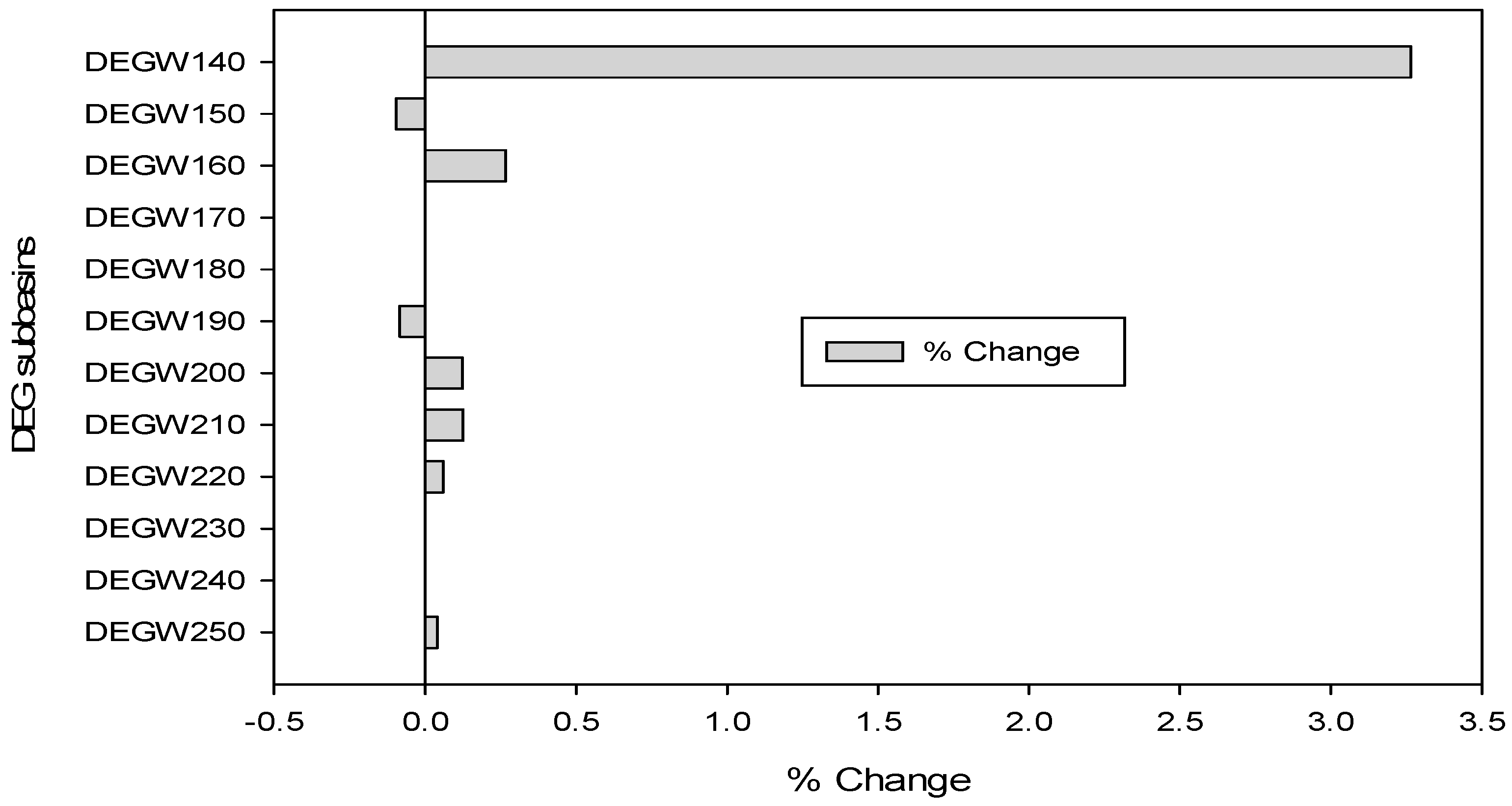
In contrast, only a few sub-basins showed increase in peak flow resulting from the Phase 1 development. For example, Table 6 show peak flow increased from about 178 m3/s to 212 m3/s and 151 to 182 m3/s in AOW40 and AOW50 respectively; however, there was no increase in peak flow in AOW60 sub-basin. Again, Table 6 show only one sub-basin (DEGW140) experienced changes in peak flow. There was no increase in peak flow in majority of the Sub-basins. Similarly, only two sub-basins (BUG 140 and PHCW210) experienced increase in peak flow due to the current project alternative.
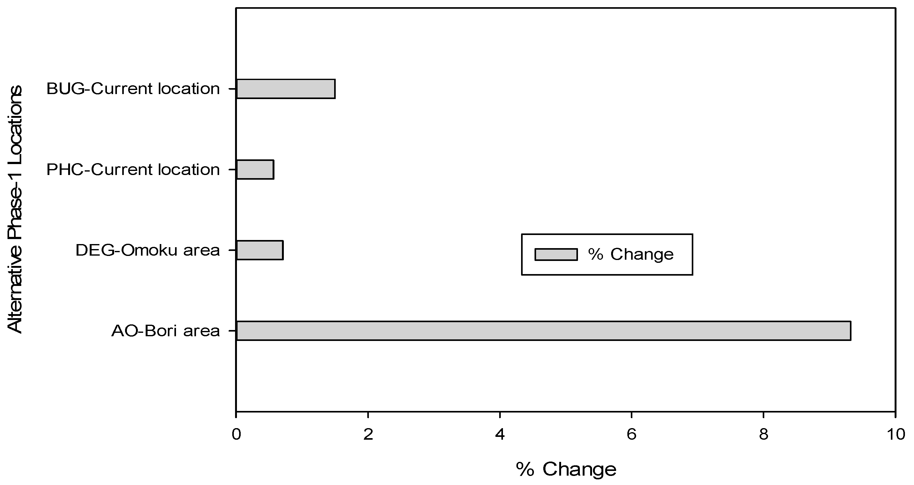
In terms of percentage change, Figure 4 demonstrates that the Bori alternative generated the highest basin scale change in peak discharge of about 9.3%, followed by the current project alternative, which caused a very slight change (of about 1.4%). The Omoku area alternative caused the least change (a negligible change of about 0.7%). Based on the result, the effect of the current project alternative was negligible, but as stated above, the Ogba-Omoku alternative was generally the least disruptive of the three location alternatives.
Figure 5, Figure 6, Figure 7 and Figure 8 compare sub-basin scale changes in peak discharge due to the project alternatives. Similarly, they demonstrate that the development in the Andoni-Ogoni Basin generated the most changes in QP followed by the development in Buguma basin. Figure 6 shows that W50 and W40 will experience the most negative change (21% and 11%) due to the Bori alternative. Moreover, the current location produced different effects in the Buguma and Port-Harcourt/Bonny Basins. About 9.0% and 5.0% change occurred in BUGW140 and PHCW210 sub-basins respectively. Meanwhile, the least change was observed in DEGW140 due to the alternative development in the Omoku/Ogba area. In general, the Omoku/Ogba alternative produced the least change, followed by the preferred or current project alternative near the old city. The Bori alternative project location produced the worst effect on runoff at the basin and sub-basin scales.
5. Discussion
Despite the scarcity of observed data in the region, the HEC-HMS model produced a reasonable performance when validated against the observed data. The results show how useful the hydrologic model is for assessing hydrologic responses and predicting future outcomes for the watershed. Validated results were found to be within the range when compared with related studies, e.g., Roy and Mistri [68] and Knebl, et al. [72]. Data scarcity remained a challenge in the study region. Based on the model performance, this study supports prior studies such as Sorrell [73] and Roy and Mistri [68] that the alternative PUB approach that rely on physically based and conceptual models are reliable for producing reasonable estimates of changes in peak flow in ungauged watersheds. However, this can be improved with the availability of observed (calibration) data.
Effects of Developmental Alternatives on Sub-Basin Hydrology
Based on the model results (Figure 4, Figure 5, Figure 6, Figure 7 and Figure 8), analysis of the relative effects of the three Phase 1 location alternatives demonstrates that the Omoku-Ogba location alternative generated the least change in peak flow. Changes due to the Omoku-Ogba and the current project location alternative were negligible. In contrast, the Bori location alternative generated the most change in peak flow even at the sub-basin scale. Note that uncertainties with the results could result from digitisation, data quality and model error itself and these could have an effect on the outcome of the analysis however, the results were deemed reliable because the model validation was reasonable. Moreover, the uncertainties were not multiplying and so they were not biased in one direction.
The result in Figure 4 mean that developments in different locations (basins) with the same spatial extent could have different effects on peak discharge in the studied watershed. The result of this study was consistent with the study by Glasson et al., [28] stated that a different location alternative is likely to generate different effects.
Other hydrological studies have suggested that the location or placement of impermeable surfaces (IS) within a basin of the watershed can have significant influence on watershed hydrology [30,31,32]. Du et al. [30] showed that an increase in the IS upstream amplified peak flow upstream 14 times more than in the downstream area in the Longhua Basin, China. In contrast the location of the Phase 1 developments did not have a significant impact on the peak flow in the basins (Figure 4). This is because the change caused by the Bori alternative (located downstream) was 13 times higher than the changes caused by the Ogba-Omoku alternative (located upstream). Hence, the magnitude of change may rather be due to the size of the basin since the effect of urbanisation was more pronounced in smaller basins. In this context, the Andoni-Ogoni basin (where the Bori alternative is located) is the smallest basin.
It is also widely acknowledged that land-use changes affect the hydrology of catchments [6,15,74,75]. From a hydrologic standpoint, placing the development in the Omoku-Ogba area would have been the least disruptive. Hence, results from the hydrologic model could be useful for decision-making in land-use planning. It could also be useful when making decisions on alternatives in the EIA and planning process. According to the South African Department of Environmental Affairs and Tourism, DEAT [35] “location alternatives are particularly relevant in change of land use applications”. Although factors such as proximity to the old city should be considered before deciding on choosing an alternative during land-use planning, results in the study supports the view in hydrology that the hydrological impact is also important. In this case, the location alternative with the least impact on peak flow should be selected.
From a hydrology standpoint, it is also important for planners and developers to understand the land-use dynamics in different basins. For example, the analysis (Figure 4) shows that the effect of urbanisation was greater in the Andoni-Ogoni Basin where the Bori alternative is situated than in the Buguma and Degema Basins, which is supported by the theory that the effect of urbanisation is more pronounced in smaller basins than larger ones. It is pertinent to note that the analysis and assumptions made for the alternatives applied in this study are only used for academic purposes, as decisions for the Phase 1 project have already been made. The analysis in this study was used to demonstrate the importance of hydrologic models for aiding land-use and EIA decision making and for understanding the implications of the position of paved surfaces in hydrology. It also helped in understanding the role location plays in the hydrology of the studied urban area. Moreover, at the sub-basin scale, findings in this study showed that the greatest changes in peak discharge were observed in sub-basins where developments were sited. For example, Figure 5 revealed that AOW40 and AOW50 experienced the most changes in the Andoni-Ogoni basin.
Based on the findings in this study (Figure 5, Figure 6, Figure 7 and Figure 8), severe and frequent flooding are some of the main concerns due to increased peak discharge in sub-basins. The indication that urbanisation is expected to have adverse effects on sub-basin peak flow suggest more people may become vulnerable to frequent flooding. This study recommends that planning and watershed management should be carried out on a sub-basin-by-sub-basin basis. Therefore, areas predicted to experience increased peak flow should be a priority for flood risk management. Increased runoff and frequent flooding due to urbanisation may accelerate soil erosion by dislodging and transporting sediments, especially in areas with sparse vegetation [74]. This process may also reduce the penetration of light into water due to increased turbidity. Soil erosion may eventually lead to reduction of productivity in upland areas and increased sedimentation in downstream areas [76].
6. Conclusions
The purpose of this research was to understand the relative effect of the EIA location alternatives (in three different locations on the urban hydrology of the GPH watershed. The study generally found that the Omoku-Ogba alternative had the least impact on runoff. That is Omoku-Ogba instead the preferred Port-Harcourt alternative could have been the least disruptive alternative. The Bori alternative could have been the most disruptive compared to the Omoku-Ogba and current project alternative. This implies that developments with the same spatial extent could generate different effects in sub-basins in the studied area. This trend is the same for the sub-basin scale changes and is consistent with the view of Glasson [50] who noted in their study that different alternatives are likely to generate different effects.
This study has furthered knowledge by showing that placement of impermeable surface (whether upstream or downstream) is probably not the main factor affecting flow in the studied watershed, instead basin size is likely the main factor influencing runoff. This conclusion was based on the finding that the smallest basin (Andoni-Ogoni Basin) experienced the greatest change.
In conclusion, examination of the three location alternatives showed that the Bori location alternative situated in the smallest basin could have been the most disruptive instead of the selected alternative. This buttresses the point that hydrology should be an important factor apart from proximity when making planning decisions. From a hydrological standpoint, urbanization could have a greater effect in smaller basins in the area. The study also finds that placement of a development had considerable effect on the peak flow at the basin scale Therefore, planning should be carried out on a sub-basin-by-sub-basin basis to effectively reduce the risk of flooding. Finally, greater attention should be paid to smaller sub-basins such as AWO 50 and AWO 40.
Despite the lack of adequate data for study in the area, model estimates were deemed dependable because it showed reasonable performance when validated with available observed data. This research successfully attempted to provide reliable estimates of changes in peak flow in the studied watershed, however, accuracy of future modelling can be improved using observed data, where available for the purpose of model calibration and validation and LiDAR data for a more accurate representation of basin characteristics.
Author Contributions
Conceptualization, N.G.D.-J. and M.J.M.; Methodology, N.G.D.-J.; Writing—Original Draft Preparation, N.G.D.-J. and M.J.M.; Writing—Review & Editing, N.G.D.-J.; Supervision, M.J.M.
Funding
This research received no external funding.
Acknowledgments
The authors’ wishes to acknowledge the assistance of Rivers State Sustainable Development Agency for funding the PhD program and the Greater Port-Harcourt Development Authority for issuing some input data used in the analysis. We also wish to thank other contributors for their effort, time and generosity of spirit, especially to Meriwether Wilson for her supervisory role and Owen McDonald for his technical assistance.
Conflicts of Interest
The authors declare no conflict of interest.
References
- IFRC. World Disasters Report: Focus on Culture and Risk; IFRC: Geneva, Switzerland, 2014. [Google Scholar]
- Jha, A.K.; Bloch, R.; Lamond, J. Cities and Flooding: A Guide to Integrated Urban Flood Risk Management for the 21st Century; World Bank Publications: Washinghton, DC, USA, 2012. [Google Scholar]
- Cho, S.-H.; Kim, H.; Roberts, R.K.; Kim, T.; Lee, D. Effects of changes in forestland ownership on deforestation and urbanization and the resulting effects on greenhouse gas emissions. J. For. Econ. 2014, 20, 93–109. [Google Scholar] [CrossRef]
- Du, J.; Qian, L.; Rui, H.; Zuo, T.; Zheng, D.; Xu, Y.; Xu, C.Y. Assessing the effects of urbanization on annual runoff and flood events using an integrated hydrological modeling system for Qinhuai River basin, China. J. Hydrol. 2012, 464, 127–139. [Google Scholar] [CrossRef]
- Hejazi, M.I.; Markus, M. Impacts of urbanization and climate variability on floods in Northeastern Illinois. J. Hydrol. Eng. 2009, 14, 606–616. [Google Scholar] [CrossRef]
- Hollis, G.E. The effect of urbanization on floods of different recurrence interval. Water Resour. Res. 1975, 11, 431–435. [Google Scholar] [CrossRef]
- Islam, T.; Ryan, J. Chapter 3-The Role of Governments in Hazard Mitigation. In Hazard Mitigation in Emergency Management; Islam, T., Ryan, J., Eds.; Butterworth-Heinemann: Oxford, UK, 2016; pp. 69–100. [Google Scholar] [CrossRef]
- Elliott, A.H.; Spigel, R.H.; Jowett, I.G.; Shankar, S.U.; Ibbitt, R.P. Model application to assess effects of urbanisation and distributed flow controls on erosion potential and baseflow hydraulic habitat. Urban Water J. 2010, 7, 91–107. [Google Scholar] [CrossRef]
- Hu, S.; Zhi-mao, G.; Jun-ping, Y. The impacts of urbanization on soil erosion in the Loess Plateau region. J. Geogr. Sci. 2001, 11, 282–290. [Google Scholar] [CrossRef]
- Putro, B.; Kjeldsen, T.R.; Hutchins, M.G.; Miller, J. An empirical investigation of climate and land-use effects on water quantity and quality in two urbanising catchments in the southern United Kingdom. Sci. Total Environ. 2016, 548, 164–172. [Google Scholar] [CrossRef] [PubMed]
- Tu, M.-C.; Smith, P.; Filippi, A.M. Hybrid forward-selection method-based water-quality estimation via combining Landsat TM, ETM+, and OLI/TIRS images and ancillary environmental data. PLoS ONE 2018, 13, e0201255. [Google Scholar] [CrossRef]
- Sanderson, D.; Sharma, A. World Disasters Report 2016. In Resilience: Saving Lives Today, Investing for Tomorrow; International Federation of Red Cross and Red Crescent Societies: Geneva, Switzerland, 2016. [Google Scholar]
- Tang, Z.; Engel, B.A.; Pijanowski, B.C.; Lim, K.J. Forecasting land use change and its environmental impact at a watershed scale. J. Environ. Manag. 2005, 76, 35–45. [Google Scholar] [CrossRef] [PubMed]
- Baloch, M.A.; Ames, D.P.; Tanik, A. Hydrologic impacts of climate and land-use change on Namnam Stream in Koycegiz Watershed, Turkey. Int. J. Environ. Sci. Technol. 2015, 12, 1481–1494. [Google Scholar] [CrossRef]
- Leopold, L. Hydrology for Urban Planning; US Geological Survey: Washington, DC, USA, 1968.
- Lazaro, T.R. Urban Hydrology; Revised Edition; CRC Press: Boca Raton, FA, USA, 1990. [Google Scholar]
- Booth, D.B. Urbanization and the Natural Drainage System--Impacts, Solutions, and Prognoses. Northwest Environ. J. 1991, 7, 93–118. [Google Scholar]
- Pauleit, S.; Duhme, F. Assessing the environmental performance of land cover types for urban planning. Landsc. Urban Plan. 2000, 52, 1–20. [Google Scholar] [CrossRef]
- Wheater, H.; Evans, E. Land use, water management and future flood risk. Land Use Policy 2009, 26, S251–S264. [Google Scholar] [CrossRef]
- Sadler, B. International Study of the Effectiveness of Environmental Assessment; IAIA: Santa Fe, Mexico, 1996; p. 263. [Google Scholar]
- Glasson, J.; Salvador, N.N.B. EIA in Brazil: A procedures–practice gap. A comparative study with reference to the European Union, and especially the UK. Environ. Impact Assess. Rev. 2000, 20, 191–225. [Google Scholar] [CrossRef]
- Mondal, M.K.; Dasgupta, B.V. EIA of municipal solid waste disposal site in Varanasi using RIAM analysis. Resour. Conserv. Recycl. 2010, 54, 541–546. [Google Scholar] [CrossRef]
- Wood, C. Environmental Impact Assessment in Developing Countries. Int. Dev. Plan. Rev. 2013, 25. [Google Scholar] [CrossRef]
- Saddler, B. Environmental Assessment in a Changing World: Evaluating Practice to Improve Performance; Canadian Environmental Assessment Agency: Ottawa, ON, Canada, 1996. [Google Scholar]
- Wood, C. Environmental Impact Assessment: A Comparative Review, 2nd ed.; Pearson Education Limited: London, UK, 2003. [Google Scholar]
- UNECA. Review of the Application of Environmental Impact Assessment in Selected African Countries; Economic Commission for Africa: Addis Ababa, Ethiopia, 2005. [Google Scholar]
- Morgan, R.K. Environmental impact assessment: The state of the art. Impact Assess. Proj. Apprais. 2012, 30, 5–14. [Google Scholar] [CrossRef]
- Glasson, J.; Therivel, R.; Chadwick, A. Introduction to Environmental Impact Assessment, 3rd ed.; Routledge: Oxford, UK, 2005. [Google Scholar]
- Ewing, R.H. Characteristics, causes, and effects of sprawl: A literature review. In Urban Ecology; Springer: Boston, MA, USA, 2008; pp. 519–535. [Google Scholar]
- Du, S.; Shi, P.; Van Rompaey, A.; Wen, J. Quantifying the impact of impervious surface location on flood peak discharge in urban areas. Nat. Hazards 2015, 76, 1457–1471. [Google Scholar] [CrossRef]
- Mejía, A.I.; Moglen, G.E. Spatial patterns of urban development from optimization of flood peaks and imperviousness-based measures. J. Hydrol. Eng. 2009, 14, 416–424. [Google Scholar] [CrossRef]
- Su, W.; Ye, G.; Yao, S.; Yang, G. Urban land pattern impacts on floods in a new district of China. Sustainability 2014, 6, 6488–6508. [Google Scholar] [CrossRef]
- Theobald, D.M.; Hobbs, N.T. A framework for evaluating land use planning alternatives: Protecting biodiversity on private land. Conserv. Ecol. 2002, 6, 5. [Google Scholar] [CrossRef]
- González, A.; Thérivel, R.; Fry, J.; Foley, W. Advancing practice relating to SEA alternatives. Environ. Impact Assess. Rev. 2015, 53, 52–63. [Google Scholar] [CrossRef]
- DEAT. Criteria for Determining Alternatives in EIA, Integrated Environmental Management; Information Series 11; Department of Environmental Affairs and Tourism: Pretoria, South Africa, 2004.
- Steinemann, A. Improving alternatives for environmental impact assessment. Environ. Impact Assess. Rev. 2001, 21, 3–21. [Google Scholar] [CrossRef]
- João, E. Key Principles of SEA. In Implementing Strategic Environmental Assessment; Schmidt, M., João, E., Albrecht, E., Eds.; Springer: Heidelberg/Berlin, Germany, 2005; Volume 2, pp. 3–14. [Google Scholar]
- Scannapieco, D.; Naddeo, V.; Belgiorno, V. Sustainable power plants: A support tool for the analysis of alternatives. Land Use Policy 2014, 36, 478–484. [Google Scholar] [CrossRef]
- Kim, S.; Ryu, Y. Describing the spatial patterns of heat vulnerability from urban design perspectives. Int. J. Sustain. Dev. World Ecol. 2015, 22, 189–200. [Google Scholar] [CrossRef]
- Nicolaisen, M.S.; Næss, P. Roads to nowhere: The accuracy of travel demand forecasts for do-nothing alternatives. Transp. Policy 2015, 37, 57–63. [Google Scholar] [CrossRef]
- Cookey-Gam, A. An Overview of the Greater portHarcourt City Master Plan and Opportunities in Building a World Class City over the Next 20Years; Greater Port-Harcourt City Development Authourity: Port Harcourt, Nigeria, 2010. [Google Scholar]
- Verml. Greater Port-Harcourt City Phase 1A Development Environmental Impact Assessment; Greater Port-Harcourt City Development Authourity: Port Harcourt, Nigeria, 2009. [Google Scholar]
- Akukwe, T.I.; Ogbodo, C. Spatial Analysis of Vulnerability to Flooding in Port Harcourt Metropolis. Nigeria. Sage Open 2015, 5. [Google Scholar] [CrossRef]
- SPDC. Environmental Impact Assessment for Afam FDP (Gas Supply) Project; The Shell Petroleum Development Company of Nigeria: Abuja, Nigeria, 2007. [Google Scholar]
- Chiadikobi, K.C.; Omoboriowo, A.O.; Chiaghanam, O.I.; Opatola, A.O.; Oyebanji, O. Flood Risk Assessment of Port Harcourt, Rivers State, Nigeria. Adv. Appl. Sci. Res. 2011, 2, 287–298. [Google Scholar]
- Ede, P.N.; Owei, O.B.; Akarolo, C.I. Does the Greater Port Harcourt Master Plan 2008 meet Aspirations for Liveable City. In Proceedings of the 47th ISOCARP Congress, Wuhan, China, 24–28 October 2011; p. 12. [Google Scholar]
- Demographia. Demographia World Urban Areas; Demographia: Belleville, IL, USA, 2017. [Google Scholar]
- Ikechukwu, E.E. The Socio-Economic Impact of the Greater Port Harcourt Development Project on the Residents of the Affected Areas. Open J. Soc. Sci. 2015, 3, 82. [Google Scholar] [CrossRef]
- Izeogu, C.V. Urban development and the environment in Port Harcourt. Environ. Urban. 1989, 1, 59–68. [Google Scholar] [CrossRef] [Green Version]
- Glasson, J.; Therivel, R.; Chadwick, A. Introduction to Environmental Impact Assessment; Routledge: Abingdon, UK, 2013. [Google Scholar]
- USDA. Hydrologic Soils Group (HSG); Natural Resources Conservation Service, United States Department of Agriculture: Washington, DC, USA, 2014; p. 1.
- Feldman. Hydrologic Modeling System HEC–HMS, Technical Reference Manual; US Army Corps or Engineers-Hydrologic Engineering Center: Washington, DC, USA, 2000.
- Roger, C. Urban hydrology for small watersheds. Tech. Release 1986, 55, 2–6. [Google Scholar]
- Yan, K.; Di Baldassarre, G.; Solomatine, D.P. Exploring the potential of SRTM topographic data for flood inundation modelling under uncertainty. J. Hydroinform. 2013, 15, 849–861. [Google Scholar] [CrossRef]
- Satgé, F.; Arsen, A.; Bonnet, M.; Timouk, F.; Calmant, S.; Pilco, R.; Molina, J.; Lavado, W.; Crétaux, J. Quality assessment of Digital Elevation Model (DEM) in view of the Altiplano hydrological modeling. In Proceedings of AGU Spring Meeting Abstracts; American Geophysical Union: Washington, DC, USA, 2013. [Google Scholar]
- Falorni, G.; Teles, V.; Vivoni, E.R.; Bras, R.L.; Amaratunga, K.S. Analysis and characterization of the vertical accuracy of digital elevation models from the Shuttle Radar Topography Mission. J. Geophys. Res. Earth Surf. 2005, 110. [Google Scholar] [CrossRef]
- Wang, W.; Yang, X.; Yao, T. Evaluation of ASTER GDEM and SRTM and their suitability in hydraulic modelling of a glacial lake outburst flood in southeast Tibet. Hydrol. Process. 2012, 26, 213–225. [Google Scholar] [CrossRef]
- Patro, S.; Chatterjee, C.; Singh, R.; Raghuwanshi, N.S. Hydrodynamic modelling of a large flood-prone river system in India with limited data. Hydrol. Process. 2009, 23, 2774–2791. [Google Scholar] [CrossRef]
- Lunetta, R.S.; Knight, J.F.; Ediriwickrema, J.; Lyon, J.G.; Worthy, L.D. Land-cover change detection using multi-temporal MODIS NDVI data. Remote Sens. Environ. 2006, 105, 142–154. [Google Scholar] [CrossRef]
- Yang, X.t.; Liu, H.; Gao, X. Land cover changed object detection in remote sensing data with medium spatial resolution. Int. J. Appl. Earth Obs. Geoinf. 2015, 38, 129–137. [Google Scholar] [CrossRef]
- Lu, D.; Mausel, P.; Brondízio, E.; Moran, E. Change detection techniques. Int. J. Remote Sens. 2004, 25, 2365–2401. [Google Scholar] [CrossRef]
- Tsui, O.W.; Coops, N.C.; Wulder, M.A.; Marshall, P.L.; McCardle, A. Using multi-frequency radar and discrete-return LiDAR measurements to estimate above-ground biomass and biomass components in a coastal temperate forest. Isprs J. Photogramm. Remote Sens. 2012, 69, 121–133. [Google Scholar] [CrossRef]
- Parent, J.R.; Volin, J.C.; Civco, D.L. A fully-automated approach to land cover mapping with airborne LiDAR and high resolution multispectral imagery in a forested suburban landscape. Isprs J. Photogramm. Remote Sens. 2015, 104, 18–29. [Google Scholar] [CrossRef]
- USACE. HEC-GeoHMS Geospatial Hydrologic MOdelling Extention: User’s Manual Version 4.2; US Army Coprs of Engineers Institute of Water REsources Hydrologic Engineering Centre: Califonia, CA, USA, 2009. [Google Scholar]
- USACE. Hydrologic Modeling System HEC-HMS: User’s Manual Version 4.0; US Army Corps of Engineers Institute for Water Centre: Califonia, CA, USA, 2013.
- Ford, D.; Pingel, N.; DeVries, J. Hydrologic Modeling System HEC-HMS: Applications Guide; US Army Corps of Engineers, Hydrologic Engineering Center: Washington, DC, USA, 2002.
- Song, X.-M.; Kong, F.-Z.; Zhu, Z.-X. Application of Muskingum routing method with variable parameters in ungauged basin. Water Sci. Eng. 2011, 4, 1–12. [Google Scholar] [CrossRef]
- Roy, S.; Mistri, B. Estimation of peak flood discharge for an ungauged river: A case study of the Kunur River, West Bengal. Geogr. J. 2013, 2013. [Google Scholar] [CrossRef]
- Lange, J.; Leibundgut, C. Non-calibrated arid zone rainfall-runoff modelling. In The Hydrology–Geomorphology Interface: RAINFALL, Floods, Sedimentation, Land Use, Proceedings of the Jerusalem Conference, Jerusalem, Israel, May 1999; IAHS Press: Wallingford, UK, 2000. [Google Scholar]
- Okoro, B.; Uzoukwu, R. Streamflow Models of Imo River for Regional Water Resources Allocation. Int. J. Eng. Sci. (IJES) 2013, 2, 97–103. [Google Scholar]
- Chai, T.; Draxler, R.R. Root mean square error (RMSE) or mean absolute error (MAE)?–Arguments against avoiding RMSE in the literature. Geosci. Model Dev. 2014, 7, 1247–1250. [Google Scholar] [CrossRef]
- Knebl, M.; Yang, Z.-L.; Hutchison, K.; Maidment, D. Regional scale flood modeling using NEXRAD rainfall, GIS, and HEC-HMS/RAS: A case study for the San Antonio River Basin Summer 2002 storm event. J. Environ. Manag. 2005, 75, 325–336. [Google Scholar] [CrossRef] [PubMed]
- Sorrell, R.C. Computing Flood Discharges for Small Ungaged Warersheds; Geological and Land Management Division, Michigan Department of Environmental Quality: Lansing, MI, USA, 2010.
- González, A.; Gilmer, A.; Foley, R.; Sweeney, J.; Fry, J. Applying geographic information systems to support strategic environmental assessment: Opportunities and limitations in the context of Irish land-use plans. Environ. Impact Assess. Rev. 2011, 31, 368–381. [Google Scholar] [CrossRef] [Green Version]
- Oleyiblo, J.O.; Li, Z. Application of HEC-HMS for flood forecasting in Misai and Wan’an catchments in China. Water Sci. Eng. 2010, 3, 14–22. [Google Scholar] [CrossRef]
- Fabricius, K.E. Effects of terrestrial runoff on the ecology of corals and coral reefs: Review and synthesis. Mar. Pollut. Bull. 2005, 50, 125–146. [Google Scholar] [CrossRef]
Figure 1.
(a) Map showing the Greater Port-Harcourt (GPH) Phase 1 location alternatives in the studied watershed. (b) Land-use/land cover layout of the GPH Master plan showing position of Phases 1, 2 and 3 areas within the new city (Source: Greater Port-Harcourt Development Authority (GPHDA), 2008).


Figure 2.
Map of the Greater Port-Harcourt watershed showing the sub-basins of the studied watershed.
Figure 2.
Map of the Greater Port-Harcourt watershed showing the sub-basins of the studied watershed.

Figure 3.
SCS unit hydrograph.

Figure 4.
Basin peak flow response to GPH Phase 1 development in three alternative locations. It shows changes due to the Bori alternative location, which was considerably higher than changes in all other basins.
Figure 4.
Basin peak flow response to GPH Phase 1 development in three alternative locations. It shows changes due to the Bori alternative location, which was considerably higher than changes in all other basins.

Figure 5.
Sub-basin peak flow response to the Phase 1 alternative in the Degema Basin. Changes in the right direction represent negative changes. It shows changes in DEG 140 were higher than changes in other sub-basins in the Degema Basin.
Figure 5.
Sub-basin peak flow response to the Phase 1 alternative in the Degema Basin. Changes in the right direction represent negative changes. It shows changes in DEG 140 were higher than changes in other sub-basins in the Degema Basin.

Figure 6.
Sub-basin peak flow response to the Phase 1 alternative in the Andoni-Ogoni Basin. Changes in the right direction represent negative changes. It shows changes in sub-basins AO W50 and AO W40 were greater than changes in the AO W60 sub-basin.
Figure 6.
Sub-basin peak flow response to the Phase 1 alternative in the Andoni-Ogoni Basin. Changes in the right direction represent negative changes. It shows changes in sub-basins AO W50 and AO W40 were greater than changes in the AO W60 sub-basin.

Figure 7.
Sub-basin peak flow response to the Phase 1 alternative in the Port-Harcourt/Bonny Basin. Changes in the right direction represent negative changes. It demonstrates that changes in peak flow due to the Phase 1 alternative was greater than changes in peak flow due to the 2003 conditions. In this basin, sub-basin PHC210 experienced the highest peak flow.

Figure 8.
Sub-basin peak flow response to the Phase 1 alternative in the Buguma Basin. Changes in the right direction represent negative changes. It demonstrates that changes in peak flow due to the Buguma alternative was greater than changes in peak flow due to the 2003 conditions. In this basin, sub-basin BUG 140 experienced the highest peak flow.


Table 1.
Hydrologic soil group classification for the study area. The area was mainly covered with HSG C (sandy clay) and HSG D (clay) soil groups.
Table 1.
Hydrologic soil group classification for the study area. The area was mainly covered with HSG C (sandy clay) and HSG D (clay) soil groups.
| FAO’s Soil Type | Texture | HSG Code | Infiltration Rate |
|---|---|---|---|
| Fluvosol | Clay | D | Very low |
| Gleysol | Clay | D | Very low |
| Ferrosol | Sandy clay | C | Low |
Table 2.
Channel geometry data comprising of channel slope, roughness (Manning’s n), channel shape, side slope and channel width (m).
Table 2.
Channel geometry data comprising of channel slope, roughness (Manning’s n), channel shape, side slope and channel width (m).
| Reaches | Length (m) | Slope | Manning | Shape | Side Slope | Width (m) |
|---|---|---|---|---|---|---|
| AO | ||||||
| R30 | 28,037 | 0.2198 | 0.05 | Triangle | 0.0522 | |
| PHC/BNY | ||||||
| R40 | 3620.7 | 0.0022 | 0.05 | Triangle | 0.667 | |
| R60 | 8782.2 | 0.0255 | 0.05 | Triangle | 0.0185 | |
| R70 | 14,350 | 0.22 | 0.05 | Rectangle | 365.71 | |
| R90 | 3888.9 | 0.041 | 0.05 | Rectangle | 1691.84 | |
| R110 | 16,016 | 0.055 | 0.05 | Rectangle | 6114.18 | |
| R150 | 130.82 | 0.002 | 0.05 | Rectangle | 3017.27 | |
| R130 | 65.409 | 0.69 | 0.05 | Rectangle | 3017.27 | |
| BUGUMA | ||||||
| R50 | 55,893 | 0.005 | 0.05 | Triangle | 0.0304 | |
| R60 | 23,343 | 0.017228 | 0.05 | Triangle | 0.042 | |
| R70 | 46.251 | 0.000025 | 0.05 | Rectangle | 364.46 | |
| R80 | 32,259 | 0.000025 | 0.05 | Trapezoid | 0.024 | 90.6 |
| DEGEMA | ||||||
| R40 | 8046.1 | 0.0022 | 0.32 | Triangle | 0.23 | |
| R60 | 11,313 | 0.225 | 0.32 | Triangle | 0.0077 | |
| R70 | 9072.9 | 0.22 | 0.05 | Triangle | 0.042 | |
| R90 | 13,852 | 0.041 | 0.05 | Triangle | 0.086 | |
| R110 | 65.409 | 0.055 | 0.05 | Rectangle | 549.66 | |
| R120 | 15,055 | 0.69 | 0.05 | Rectangle | 915 | |
Table 3.
Comparison of error functions for annual peak flows for the Imo River outlet between 1985 and 1988.
Table 3.
Comparison of error functions for annual peak flows for the Imo River outlet between 1985 and 1988.
| Year | Observed Qp (m3/s) | Estimated Qp (m3/s) | Absolute Error (AE) | Squared Error (SE) | Relative Error (RE) | Relative Percentage Error (RPE) |
|---|---|---|---|---|---|---|
| 1985 | 286.16 | 273.15 | 13.13 | 169.02 | 0.05 | 4.54 |
| 1986 | 200.02 | 279.63 | 79.61 | 6336.16 | 0.40 | 39.80 |
| 1987 | 223.20 | 255.32 | 32.10 | 1030.41 | 0.14 | 14.38 |
| 1988 | 307.81 | 280.60 | 27.23 | 739.84 | 0.09 | 8.84 |
Table 4.
Summary of model performance of estimated annual peak flows for the Imo River outlet between 1985 and 1988.
Table 4.
Summary of model performance of estimated annual peak flows for the Imo River outlet between 1985 and 1988.
| Performance Criteria | Values |
|---|---|
| MAE | 37.98 |
| RMSE | 45.49 |
| MRPE | 16.89% |
Table 5.
The modelled result for peak flow responses to the Bori alternative location in the Andoni-Ogoni Basin. AO = Andoni/Ogoni; Qp = peak discharge; Qp-2003 = peak discharge based on the 2003 LULC condition; Qp-Phase 1 Alternative = peak discharge based on Phase 1 alternative LULC condition.
Table 5.
The modelled result for peak flow responses to the Bori alternative location in the Andoni-Ogoni Basin. AO = Andoni/Ogoni; Qp = peak discharge; Qp-2003 = peak discharge based on the 2003 LULC condition; Qp-Phase 1 Alternative = peak discharge based on Phase 1 alternative LULC condition.
| Location Alternative | Host Basin Code | Sub-Basin Code | Area (km2) | Qp-2003 | Qp-Phase 1 Alternative |
|---|---|---|---|---|---|
| (m3/s) | (m3/s) | ||||
| Bori | Andoni/Ogoni Basin | AOW60 | 209.57 | 327.60 | 326.40 |
| AOW40 | 178.85 | 191.10 | 212.90 | ||
| AO W50 | 140.11 | 151.30 | 182.50 | ||
| AO Outlet | 528.531 | 650.2 | 710.8 |
Table 6.
Modelled result of peak flow responses to Port-Harcourt Alternative in DEG = Degema; Qp = Peak discharge; Qp-2003 = Peak discharge based on year 2003 LULC condition; Qp-Phase 1 Alternative = Peak discharge based on Phase 1 alternative LULC condition.
Table 6.
Modelled result of peak flow responses to Port-Harcourt Alternative in DEG = Degema; Qp = Peak discharge; Qp-2003 = Peak discharge based on year 2003 LULC condition; Qp-Phase 1 Alternative = Peak discharge based on Phase 1 alternative LULC condition.
| Location Alternative | Host Basin Code | Sub-Basin Code | Area (km2) | Qp-2003 | Qp-Phase 1 Alternative |
|---|---|---|---|---|---|
| (m3/s) | (m3/s) | ||||
| Omoku Area | Degema Basin | DEGW250 | 144.82 | 245.80 | 245.90 |
| DEGW240 | 131.27 | 208.80 | 208.80 | ||
| DEGW230 | 45.45 | 74.60 | 74.60 | ||
| DEGW220 | 86.41 | 165.00 | 165.10 | ||
| DEGW210 | 76.08 | 79.70 | 79.80 | ||
| DEGW200 | 46.20 | 80.60 | 80.70 | ||
| DEGW190 | 75.31 | 119.00 | 118.90 | ||
| DEGW180 | 61.55 | 81.70 | 81.70 | ||
| DEGW170 | 139.34 | 204.40 | 204.40 | ||
| DEGW160 | 23.33 | 37.50 | 37.60 | ||
| DEGW150 | 94.70 | 104.00 | 103.90 | ||
| DEGW140 | 247.15 | 257.30 | 265.70 | ||
| DEG Outlet | 1171.61 | 1229.8 | 1238.5 |
Table 7.
Modelled result of peak flow responses to Current Project Alternative in Port-Harcourt Basin. PHC = Port-Harcourt Basins; W = watershed; Qp = Peak discharge; Qp-2003 = Peak discharge based on year 2003 LULC condition; Qp-Phase 1 Alternative = Peak discharge based on Phase 1 alternative LULC condition.
| Location Alternative | Host Basin Code | Sub-basin Code | Area (km2) | Qp-2003 | Qp-Phase 1 Alternative |
|---|---|---|---|---|---|
| (m3/s) | (m3/s) | ||||
| Current Location | Port-Harcourt/Bonny Basin | PHCW160 | 111.71 | 107.10 | 108.50 |
| PHCW180 | 114.87 | 123.70 | 123.70 | ||
| PHCW190 | 88.42 | 123.80 | 123.80 | ||
| PHCW200 | 31.05 | 58.20 | 58.10 | ||
| PHCW210 | 114.84 | 138.90 | 146.70 | ||
| PHCW220 | 81.67 | 159.50 | 159.50 | ||
| PHCW230 | 203.95 | 168.60 | 168.40 | ||
| PHCW240 | 188.94 | 343.90 | 343.80 | ||
| PHCW250 | 90.99 | 113.60 | 113.40 | ||
| PHCW260 | 14.08 | 28.20 | 28.20 | ||
| PHCW300 | 183.80 | 345.10 | 345.10 | ||
| PHC Outlet | 1224.32 | 1476.80 | 1485.20 |
Table 8.
Modelled result of peak flow responses to Current Project Alternative in Port-Harcourt Basin.; BUG Buguma Basin; W = watershed; Qp = Peak discharge; Qp-2003 = Peak discharge based on year 2003 land use/land cover (LULC) condition; Qp-Phase 1 Alternative = Peak discharge based on Phase 1 alternative LULC condition.
| Location Alternative | Host Basin | Sub-Basin Code | Area (km2) | Qp-2003 | Qp-Phase 1 Alternative |
|---|---|---|---|---|---|
| (m3/s) | (m3/s) | ||||
| Current location | Buguma Basin | BUGW180 | 76.87 | 154.20 | 154.20 |
| BUGW160 | 178.20 | 347.80 | 347.80 | ||
| BUGW150 | 121.50 | 148.60 | 148.50 | ||
| BUGW140 | 151.76 | 126.80 | 138.60 | ||
| BUGW130 | 187.56 | 137.20 | 137.20 | ||
| BUGW120 | 344.67 | 264.20 | 264.20 | ||
| BUGW110 | 73.13 | 61.30 | 61.30 | ||
| BUGW100 | 116.70 | 110.80 | 110.80 | ||
| BUG Outlet | 1250.395 | 840.6 | 853.2 |
© 2019 by the authors. Licensee MDPI, Basel, Switzerland. This article is an open access article distributed under the terms and conditions of the Creative Commons Attribution (CC BY) license (http://creativecommons.org/licenses/by/4.0/).
Share and Cite
MDPI and ACS Style
Dan-Jumbo, N.G.; Metzger, M. Relative Effect of Location Alternatives on Urban Hydrology. The Case of Greater Port-Harcourt Watershed, Niger Delta. Hydrology 2019, 6, 82. https://doi.org/10.3390/hydrology6030082
AMA Style
Dan-Jumbo NG, Metzger M. Relative Effect of Location Alternatives on Urban Hydrology. The Case of Greater Port-Harcourt Watershed, Niger Delta. Hydrology. 2019; 6(3):82. https://doi.org/10.3390/hydrology6030082
Chicago/Turabian StyleDan-Jumbo, Nimi G., and Marc Metzger. 2019. "Relative Effect of Location Alternatives on Urban Hydrology. The Case of Greater Port-Harcourt Watershed, Niger Delta" Hydrology 6, no. 3: 82. https://doi.org/10.3390/hydrology6030082
Note that from the first issue of 2016, this journal uses article numbers instead of page numbers. See further details here.