Deep Artificial Neural Networks for the Diagnostic of Caries Using Socioeconomic and Nutritional Features as Determinants: Data from NHANES 2013–2014

 ,
,  ,
,  ,
,
Abstract
:1. Introduction
Related Work
2. Materials and Methods
2.1. Features Description
- Demographic: it provides individual, family and household level information in different topics (income of households and families, size of households and families, pregnancy status, among others).
- Dietetic: it provides detailed information on dietary intake, in order to estimate the types and amount of food and beverages consumed, in addition to estimating the intake of energy, nutrients, and other food components.
- Examination: it provides information of the health status, indicators of disease risk, and access to preventive and treatment services, from different aspects, including oral health.
- Laboratory: it provides information of the results obtained from laboratory analysis of different components (components of urine, proteins, triglycerides, plasma, among others).
- Questionnaire: it provides information of the data obtained from the interviews conducted through a system of computer-aided personal interview, of different topics (alcohol use, cardiovascular health, dermatology, among others).
- Limited access: it provides similar information to that found in the questionnaire; however, it isn’t publicly available.
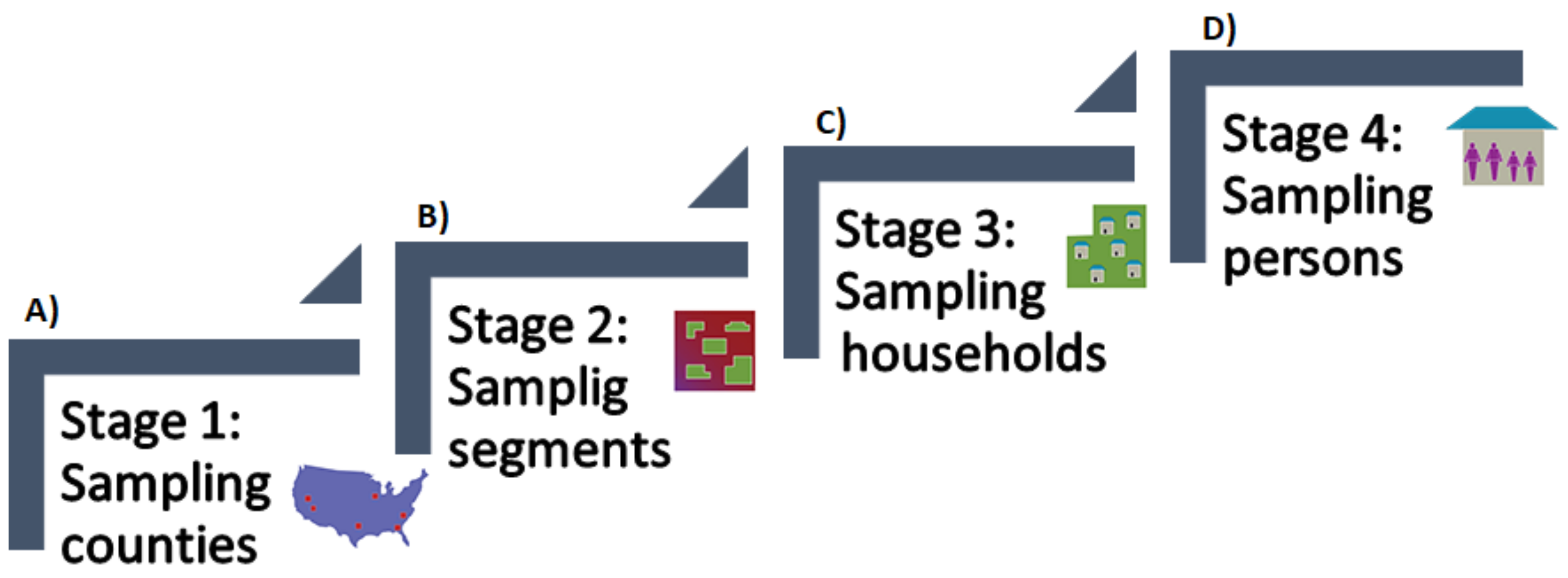
2.2. Subjects Description
- Hispanic persons;
- Non-Hispanic black persons;
- Non-Hispanic Asian persons;
- Non-Hispanic white and other* persons at or below 130% of the poverty level; and
- Non-Hispanic white and other* persons aged 80 years and older.
2.3. Data Analysis
2.3.1. Data Preprocessing
2.3.2. Data Classification
2.3.3. Evaluation
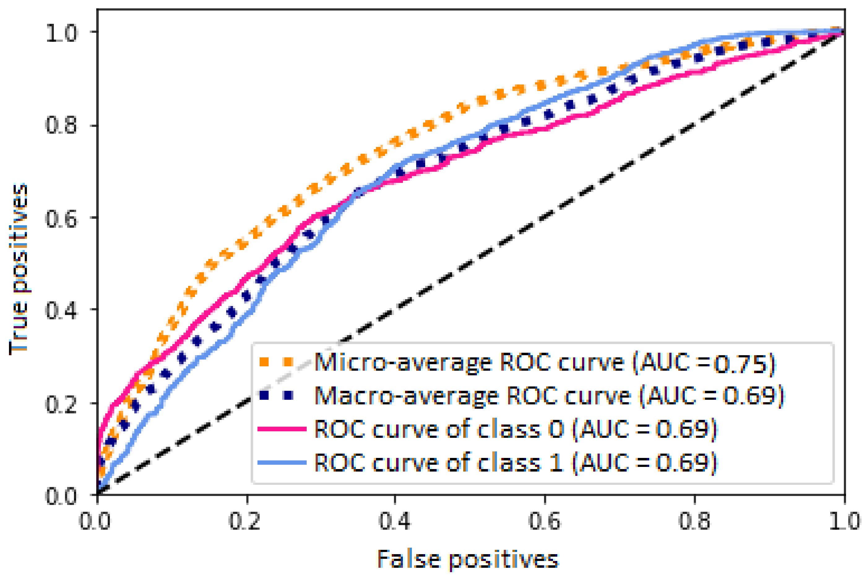
3. Results
4. Discussion
5. Conclusions
Author Contributions
Funding
Conflicts of Interest
Appendix A

| Feature | Description |
|---|---|
| AIALANGA | Language of the MEC ACASI Interview Instrument. |
| DMDBORN4 | In what country was Sample Person (SP) born? |
| DMDCITZN | Is SP a citizen of the United States? |
| DMDHHSIZ | Total number of people in the Household. |
| DMDHHSZE | Number of adults aged 60 years or older in the household. |
| DMDEDUC2 | Highest grade or level of school completed or the highest degree received. |
| DMDHHSZB | Number of children aged 6–17 years old in the household (HH). |
| DMDHSEDU | HH reference person’s spouse’s education level. |
| DMDMARTL | Marital status. |
| DMDFMSIZ | Total number of people in the Family. |
| DMDHHSZA | Number of children aged 5 years or younger in the household. |
| DMDHRGND | HH reference person’s gender. |
| DMDHREDU | HH reference person’s education level. |
| DMDEDUC3 | Highest grade or level of school completed or the highest degree received. |
| DMDHRAGE | HH reference person’s age in years. |
| DMDHRBR4 | HH reference person’s country of birth. |
| DMDHREDU | HH reference person’s education level. |
| DMDHRMAR | HH reference person’s marital status. |
| DMQADFC | Did SP ever serve in a foreign country during a time of armed conflict or on a humanitarian or peace-keeping mission? |
| DMDYRSUS | Length of time the participant has been in the US. |
| DMQMILIZ | Has SP ever served on active duty in the U.S. Armed Forces, military Reserves, or National Guard? |
| FIAINTRP | Was an interpreter used to conduct the Family interview? |
| FIALANG | Language of the Family Interview Instrument. |
| FIAPROXY | Was a Proxy respondent used in conducting the Family Interview? |
| INDFMPIR | A ratio of family income to poverty guidelines. |
| INDHHIN2 | Total household income (reported as a range value in dollars). |
| INDFMIN2 | Total family income (reported as a range value in dollars). |
| LATVPSU | Variance unit: PSU variable for variance estimation. |
| LATVSTRA | Variance unit: stratum variable for variance estimation. |
| MIAINTRP | Was an interpreter used to conduct the MEC CAPI interview? |
| MIALANG | Language of the MEC CAPI Interview Instrument. |
| MIAPROXY | Was a Proxy respondent used in conducting the MEC CAPI Interview? |
| RIAGENDR | Gender of the participant. |
| RIDAGEEX | Age in years of the participant at the time of examination. Individuals aged 959 months and older are topcoded at 959 months. |
| RIDAGEMN | ge in months of the participant at the time of screening. Reported for persons aged 24 months or younger at the time of exam. |
| RIDRETH3 | Recode of reported race and Hispanic origin information, with Non-Hispanic Asian Category. |
| RIDEXMON | Six month time period when the examination was performed. |
| RIDEXPRG | Pregnancy status for females between 20 and 44 years of age at the time of MEC exam. |
| RIDAGEYR | Age in years of the participant at the time of screening. |
| RIDRETH1 | Recode of reported race and Hispanic origin information. |
| RIDEXAGM | Age in months of the participant at the time of examination. |
| RIDSTATR | Interview and examination status of the participant. |
| SDMVPSU | Masked variance unit pseudo-PSU variable for variance estimation. |
| SDDSRVYR | Data release cycle. |
| SDMVSTRA | Masked variance unit pseudo-stratum variable for variance estimation. |
| WTLAF8YR | Subsample 8-year fasting weight for participants aged 12 years and older who were examined in the morning sessions in Los Angeles, CA, USA. |
| WTLAI8YR | Full sample 8-year interview weight for participants in Los Angeles, CA, USA. |
| WTLAM8YR | Full sample 8-year MEC exam weight for participants in Los Angeles, CA, USA. |
Appendix B
| Feature | Description |
|---|---|
| WTDRD1 | Dietary day one sample weight. |
| DBQ095Z | Type of salt usually add to food at the table. |
| DR1TKCAL | Energy (kcal). |
| DR1TSUGR | Total sugars (g). |
| DR1TFIBE | Dietary fiber (g). |
| DR1TSFAT | Total saturated fatty acids (g). |
| DR1TMFAT | Total monounsaturated fatty acids (g). |
| DR1TPFAT | Total polyunsaturated fatty acids (g). |
| DR1TLYCO | Lycopene (g). |
| DR1TFA | Folic acid (g). |
| DR1TB12A | Added vitamin B12 (g). |
| DR1_300 | Was the amount of food that you ate yesterday much more than usual, usual, or much less than usual? |
| DR1_320Z | Total plain water drank yesterday—including plain tap water, water from a drinking fountain, water from a water cooler, bottled water, and spring water. |
| DR1_330Z | Total tap water drank yesterday—including filtered tap water and water from a drinking fountain. |
| DR1BWATZ | Total bottled water drank yesterday (g). |
| DR1DAY | Intake day of the week. |
| DR1DBIH | Number of days between intake day and the day of family questionnaire administered in the household. |
| DR1SKY | What type of salt was it? (Was it ordinary or seasoned salt, lite salt, or a salt substitute?). |
| DR1STY | Did SP add any salt to her/his food at the table yesterday? |
| DR1TACAR | Alpha-carotene (g). |
| DR1TBCAR | Beta-carotene (g). |
| DR1TCAFF | Caffeine (mg). |
| DR1TCALC | Calcium (mg). |
| DR1TCOPP | Copper (mg). |
| DR1TCRYP | Beta-cryptoxanthin (g). |
| DR1TFDFE | Folate as dietary folate equivalents (g). |
| DR1TFF | Food folate (g). |
| DR1TFOLA | Total folate (g). |
| DR1TLZ | Lutein + zeaxanthin (g). |
| DR1TM161 | MFA 16:1 (Hexadecenoic) (g). |
| DR1TM181 | MFA 18:1 (Octadecenoic) (g). |
| DR1TM201 | MFA 20:1 (Eicosenoic) (g). |
| DR1TM221 | MFA 22:1 (Docosenoic) (g). |
| DR1TMAGN | Magnesium (mg). |
| DR1TMOIS | Moisture (g). |
| DR1TNIAC | Niacin (mg). |
| DR1TNUMF | Total number of foods/beverages reported in the individual foods file. |
| DR1TP182 | PFA 18:2 (Octadecadienoic) (g). |
| DR1TP183 | PFA 18:3 (Octadecatrienoic) (g). |
| DR1TP184 | PFA 18:4 (Octadecatetraenoic) (g). |
| DR1TP204 | PFA 20:4 (Eicosatetraenoic) (g). |
| DR1TP205 | PFA 20:5 (Eicosapentaenoic) (g). |
| DR1TP225 | PFA 22:5 (Docosapentaenoic) (g). |
| DR1TP226 | PFA 22:6 (Docosahexaenoic) (g). |
| DR1TPOTA | Potassium (mg). |
| DR1TRET | Retinol (g). |
| DR1TS040 | SFA 4:0 (Butanoic) (g). |
| DR1TS060 | SFA 6:0 (Hexanoic) (g). |
| DR1TS100 | SFA 10:0 (Decanoic) (g). |
| DR1TS120 | SFA 12:0 (Dodecanoic) (g). |
| DR1TS140 | SFA 14:0 (Tetradecanoic) (g). |
| DR1TS180 | SFA 18:0 (Octadecanoic) (g). |
| DR1TSELE | Selenium (g). |
| DR1TSODI | Sodium (mg). |
| DR1TTHEO | Theobromine (mg). |
| DR1TVARA | Vitamin A as retinol activity equivalents (g). |
| DR1TVB1 | Thiamin (Vitamin B1) (mg). |
| DR1TVB12 | Vitamin B12 (g). |
| DR1TVB2 | Riboflavin (Vitamin B2) (mg). |
| DR1TVB6 | Vitamin B6 (mg). |
| DR1TVC | Vitamin C (mg). |
| DR1TVK | Vitamin K (g). |
| Feature | Description |
|---|---|
| DR1TWS | When you drink tap water, what is the main source of the tap water? Is the city water supply; a well or rain cistern; a spring; or something else? |
| DR1TZINC | Zinc (mg). |
| DRABF | Indicates whether the sample person was an infant who was breast-fed on either of the two recall days. |
| DRD340 | During the past 30 days did you eat any types of shellfish listed on this card? |
| DRD350A | Clams eaten during the past 30 days. |
| DRD350AQ | Number of times clams were eaten in the past 30 days. |
| DRD350B | Crabs eaten during the past 30 days. |
| DRD350BQ | Number of times crab was eaten in the past 30 days. |
| DRD350C | Crayfish eaten during the past 30 days. |
| DRD350CQ | Number of times crayfish was eaten in the past 30 days. |
| DRD350D | Lobsters eaten during the past 30 days. |
| DRD350DQ | Number of times lobster was eaten in the past 30 days. |
| DRD350E | Mussels eaten during the past 30 days. |
| DRD350EQ | Number of times mussels were eaten in the past 30 days. |
| DRD350F | Oysters eaten during the past 30 days. |
| DRD350FQ | Number of times oysters were eaten in the past 30 days. |
| DRD350G | Scallops eaten during the past 30 days. |
| DRD350GQ | Number of times scallops were eaten in the past 30 days. |
| DRD350H | Shrimp eaten during the past 30 days. |
| DRD350HQ | Number of times shrimp was eaten in the last 30 days. |
| DRD350I | Other shellfish ( ex. octopus, squid) eaten during the past 30 days. |
| DRD350IQ | Number of times other shellfish (ex. octopus, squid) was eaten in the past 30 days. |
| DRD350J | Other unknown shellfish eaten during the past 30 days. |
| DRD350JQ | Number of times other unknown shellfish was eaten in the past 30 days. |
| DRD350K | Refused to give detailed information on shellfish eaten during the past 30 days. |
| DRD360 | During the past 30 days did you eat any types of fish listed on this card? |
| DRD370A | Breaded fish products eaten during the past 30 days. |
| DRD370AQ | Number of times breaded fish products were eaten in the past 30 days. |
| DRD370B | Tuna eaten during the past 30 days. |
| DRD370BQ | Number of times tuna was eaten in the past 30 days. |
| DRD370C | Bass eaten during the past 30 days. |
| DRD370CQ | Number of times bass was eaten in the past 30 days. |
| DRD370D | Catfish eaten during the past 30 days. |
| DRD370DQ | Number of times catfish was eaten in the past 30 days. |
| DRD370E | Cod eaten during the past 30 days. |
| DRD370EQ | Number of times cod was eaten in the past 30 days. |
| DRD370F | Flatfish eaten during the past 30 days. |
| DRD370FQ | Number of times flatfish was eaten in the past 30 days. |
| DRD370G | Haddock eaten during the past 30 days. |
| DRD370GQ | Number of times haddock was eaten in the past 30 days. |
| DRD370H | Mackerel eaten during the past 30 days. |
| DRD370HQ | Number of times mackerel was eaten in the past 30 days. |
| DRD370I | Perch eaten during the past 30 days. |
| DRD370IQ | Number of times perch was eaten in the past 30 days. |
| DRD370J | Pike eaten during the past 30 days. |
| DRD370JQ | Number of times pike was eaten in the past 30 days. |
| DRD370K | Pollock eaten during the past 30 days. |
| DRD370KQ | Number of times pollock was eaten in the past 30 days. |
| DRD370TQ | Number of times other type of fish was eaten in the past 30 days. |
| DRD370V | Refused to give detailed information on fish eaten during the past 30 days. |
| DRQSDIET | Are you currently on any kind of diet, either to lose weight or for some other health-related reason? |
| DRQSDT1 | What kind of diet are you on? (Is it a weight loss or a low calorie diet: low fat or cholesterol diet; low salt or sodium diet; sugar free or low sugar diet; low fiber diet; high fiber diet; diabetic diet; or another type of diet?). |
| DRD370L | Porgy eaten during the past 30 days. |
| DRD370LQ | Number of times porgy was eaten in the past 30 days. |
| DRD370M | Salmon eaten during the past 30 days. |
| DRD370MQ | Number of times salmon was eaten in the past 30 days. |
| DRD370N | Sardines eaten during the past 30 days. |
| DRD370NQ | Number of times sardines were eaten in the past 30 days. |
| DRD370O | Sea bass eaten during the past 30 days. |
| DRD370OQ | Number of times sea bass was eaten in the past 30 days. |
| DRD370U | Other unknown type eaten during the past 30 days. |
| Feature | Description |
|---|---|
| WTDR2D | Dietary two-day sample weight. |
| DR1DRSTZ | Dietary recall status. |
| DR1TPROT | Protein (g). |
| DR1TCARB | Carbohydrate (g). |
| DR1TTFAT | Total fat (g). |
| DR1TCHOL | Cholesterol (mg). |
| DR1TFA | Folic acid (g). |
| DR1TCHL | Total choline (mg). |
| DR1TIRON | Iron (mg). |
| DBD100 | Frequency with which ordinary salt is added to the food on the table. |
| DRQSPREP | Frequency with which ordinary salt or seasoned salt is added in cooking or preparing foods in the household. |
| DR1TALCO | Alcohol (g). |
| DR1TS080 | SFA 8:0 (Octanoic) (g). |
| DR1TATOC | Vitamin E as alpha-tocopherol (mg). |
| DR1TATOA | Added alpha-tocopherol (Vitamin E) (mg). |
| DR1TVD | Vitamin D (D2 + D3) (g). |
| DR1TPHOS | Phosphorus (mg). |
| DR1TS160 | SFA 16:0 (Hexadecanoic) (g). |
| DRD370UQ | Number of times other unknown type of fish was eaten in the past 30 days. |
| DRD370V | Refused to give detailed information on fish eaten during past 30 days. |
| DRDINT | Indicates whether the sample person has intake data for one or two days. |
| DRQSDIET | Are you currently on any kind of diet, either to lose weight or for some other health-related reason? |
References
- Oral Health. Available online: http://www.who.int/oral_health/disease_burden/global/en/ (accessed on 5 June 2017).
- Ridao Marín, D. Desarrollo de un Sistema de Ayuda a la Decisión para Tratamientos Odontológicos con Imágenes Digitales; Universidad de Málaga: Málaga, Spain, 2017; pp. 10–12. [Google Scholar]
- Espinoza Solano, M.; León-Manco, R.A. Prevalencia y experiencia de caries dental en estudiantes según facultades de una universidad particular peruana. Rev. Estomatol. Hered. 2015, 25, 187–193. [Google Scholar] [CrossRef]
- Acuña Aguilar, L.D.; Porras Cerón, D.; Ríos Rueda, L.D. Prevalencia de Lesiones Cariosas y Factores Asociados Presentes en Pacientes con SíNdrome de Down en las Fundaciones Fundown y san Luis Guanella de Bucaramanga; Universidad Santo Tomás: Bucaramanga, Colombia, 2017; pp. 12–16. [Google Scholar]
- Gispert Abreu, E.D.L.Á.; Castell-Florit Serrate, P.; Herrera Nordet, M. Salud bucal poblacional y su producción intersectorial. Rev. Cubana Estomatol. 2015, 52, 62–67. [Google Scholar]
- Niño, T.C.; Guevara, S.V.; González, F.A.; Jaque, R.A.; Infante, C. Uso de redes neuronales articiales en predicción de morfología mandibular a través de variables craneomaxilares en una vista posteroanterior. Univ. Odontol. 2016, 35, 1–28. [Google Scholar]
- Lam, C.U.; Khin, L.; Kalhan, A.; Yee, R.; Lee, Y.; Chong, M.F.; Kwek, K.; Saw, S.; Godfrey, K.; Chong, Y.; et al. Identification of Caries Risk Determinants in Toddlers: Results of the GUSTO Birth Cohort Study. Caries Res. 2017, 51, 271–282. [Google Scholar] [CrossRef] [PubMed] [Green Version]
- Fernandes, I.; Sá-Pinto, A.; Marques, L.S.; Ramos-Jorge, J.; Ramos-Jorge, M. Maternal identification of dental caries lesions in their children aged 1–3 years. Eur. Arch. Paediatr. Dent. 2017, 18, 197–202. [Google Scholar] [CrossRef] [PubMed]
- Lips, A.; Antunes, L.S.; Antunes, L.A.; Pintor, A.V.B.; Santos, D.A.B.D.; Bachinski, R.; Küchler, E.C.; Alves, G.G. Salivary protein polymorphisms and risk of dental caries: A systematic review. Braz. Oral Res. 2017, 31. [Google Scholar] [CrossRef] [PubMed]
- Ahmed, A.; Ikram, K.; Masood, H.; Urooj, M. Identification of relationship between oral disorders & hemodynamic parameters. Pak. Oral Dent. J. 2017, 37, 202–204. [Google Scholar]
- Sarmiento, R.V.; Barrionuevo, F.P.; Huamán, Y.S.; Loyola, M.C. Prevalencia de caries de infancia temprana en niños menores de 6 años de edad, residentes en poblados urbano marginales de Lima Norte. Rev. Estomatol. Herediana 2011, 21, 79–86. [Google Scholar] [CrossRef]
- Oropeza-Oropeza, C.D.; Molina-Frechero, N.; Castañeda-Castaneira, E.; Zaragoza-Rosado, C.D.; Cruz Leyva, C.D. Caries dental en primeros molares permanentes de escolares de la delegación Tláhuac. Rev. ADM 2012, 69, 63–68. [Google Scholar]
- Cardozo, B.J.; Gonzalez, M.M.; Pérez, S.R.; Vaculik, P.A.; Sanz, E.G. Epidemiología de la caries dental en niños del Jardín de Infantes “Pinocho” de la ciudad de Corrientes. Rev. Fac. Odontol. 2017, 9, 35–41. [Google Scholar]
- Zhang, X.; Zhang, L.; Zhang, Y.; Liao, Z.; Song, J. Predicting trend of early childhood caries in mainland China: A combined meta-analytic and mathematical modelling approach based on epidemiological survey. Sci. Rep. 2017, 7, 6507. [Google Scholar] [CrossRef] [PubMed]
- Asif, S.M.; Babu, D.B.; Naheeda, S. Utility of Dermatoglyphic Pattern in Prediction of Caries in Children of Telangana Region, India. J. Contemp. Dent. Pract. 2017, 18, 490–496. [Google Scholar] [CrossRef] [PubMed]
- Chapple, I.L.; Bouchard, P.; Cagetti, M.G.; Campus, G.; Carra, M.C.; Cocco, F.; Nibali, L.; Hujoel, P.; Laine, M.L.; Lingstrom, P.; et al. Interaction of lifestyle, behaviour or systemic diseases with dental caries and periodontal diseases: Consensus report of group 2 of the joint EFP/ORCA workshop on the boundaries between caries and periodontal diseases. J. Clin. Periodontol. 2017, 44, s39–s51. [Google Scholar] [CrossRef] [PubMed]
- Hayes, M.; Da Mata, C.; Cole, M.; McKenna, G.; Burke, F.; Allen, P.F. Risk indicators associated with root caries in independently living older adults. J. Dent. 2016, 51, 8–14. [Google Scholar] [CrossRef] [PubMed]
- Sudhir, K.M.; Kanupuru, K.K.; Fareed, N.; Mahesh, P.; Vandana, K.; Chaitra, N.T. CAMBRA as a Tool for Caries Risk Prediction Among 12-to 13-year-old Institutionalised Children-A Longitudinal Follow-up Study. Oral Health Prev. Dent. 2016, 14, 355–362. [Google Scholar] [PubMed]
- Twetman, S. Caries risk assessment in children: How accurate are we? Eur. Arch. Paediatr. Dent. 2016, 17, 27–32. [Google Scholar] [CrossRef] [PubMed]
- National Health and Nutrition Examination Survey Data. 2013–2014. Available online: http://www.cdc.gov/nchs/nhanes.htm (accessed on 5 November 2017).
- Zanella-Calzada, L.A.; Galván-Tejada, C.E.; Chávez-Lamas, N.M.; Gracia-Cortés, M.D.C.; Moreno-Báez, A.; Arceo-Olague, J.G.; Celaya-Padilla, J.M.; Galván-Tejada, J.I.; Gamboa-Rosales, H. A Case–Control Study of Socio-Economic and Nutritional Characteristics as Determinants of Dental Caries in Different Age Groups, Considered as Public Health Problem: Data from NHANES 2013–2014. Int. J. Environ. Res. Public Health 2018, 15, 957. [Google Scholar] [CrossRef] [PubMed]
- Zanella-Calzada, L.A.; Galván-Tejada, C.E.; Chávez-Lamas, N.M.; Galván-Tejada, J.I.; Celaya-Padilla, J.M. Multivariate features selection from demographic and dietary descriptors as caries risk determinants in oral health diagnosis: Data from NHANES 2013–2014. In Proceedings of the International Conference on Electronics, Communications and Computers (CONIELECOMP), Cholula, Mexico, 21–23 Feburary 2018; pp. 217–224. [Google Scholar]
- Chávez-Lamas, N.M.; Zanella-Calzada, L.A.; Galván-Tejada, C.E. An Analysis of Dietary and Demographic Data in Oral Health, Data from the National Health and Nutrition Examination Survey: A Preliminary Study. Adv. Comput. Netw. Appl. 2017, 142, 79–88. [Google Scholar]
- Liaw, A.; Wiener, M. Classication and regression by randomforest. R News 2002, 2, 18–22. [Google Scholar]
- Chollet, F. Keras: Deep Learning Library for Theano and Tensorflow. pp. 145–151. Available online: https://keras.io/k (accessed on 5 May 2018).
- Lomuscio, A.; Maganti, L. An approach to reachability analysis for feed-forward relu neural networks. arXiv, 2017; arXiv:1706.07351. [Google Scholar]
- Carlini, N.; Wagner, D. Towards evaluating the robustness of neural networks. In Proceedings of the IEEE Symposium on Security and Privacy (SP), San Jose, CA, USA, 22–26 May 2017; pp. 39–57. [Google Scholar]
- Kingma, D.P.; Ba, J. Adam: A method for stochastic optimization. arXiv, 2014; arXiv:1412.6980. [Google Scholar]
- Haykin, S.S. Neural Networks and Learning Machines; Pearson: Upper Saddle River, NJ, USA, 2009; Volume 3, pp. 1–46. [Google Scholar]
- Chollet, F. Deep Learning with Python; Manning Publications Co.: Greenwich, CT, USA, 2017; Volume 1, pp. 1–93. [Google Scholar]
- Antona Cortés, C. Herramientas Modernas en Redes Neuronales: La LibreríA Keras. Bachelor’s Thesis, UAM, Departamento de Ingeniería Informática, Madrid, Spain, 2017; pp. 21–38. [Google Scholar]
- Helene Bischel, S. El método de la EntropíA Cruzada. Algunas Aplicaciones. Master’s Thesis, Universidad de Almería, Almería, Spain, 2015; pp. 4–14. [Google Scholar]
- Nye, M.; Saxe, A. Are Efficient Deep Representations Learnable? UAM, Departamento de Ingeniería Informática: Madrid, Spain, 2017; pp. 1–4. [Google Scholar]
- Lobo, J.M.; Jiménez-Valverde, A.; Real, R. AUC: A misleading measure of the performance of predictive distribution models. Glob. Ecol. Biogeogr. 2008, 17, 145–151. [Google Scholar] [CrossRef]
- Hanley, J.A.; McNeil, B.J. The meaning and use of the area under a receiver operating characteristic (ROC) curve. Radiology 1982, 143, 29–36. [Google Scholar] [CrossRef] [PubMed]
- Pedregosa, F.; Varoquaux, G.; Gramfort, A.; Michel, V.; Thirion, B.; Grisel, O.; Blondel, M.; Prettenhofer, P.; Weiss, R.; Dubourg, V.; et al. Scikit-learn: Machine learning in Python. J. Mach. Learn. Res. 2011, 12, 2825–2830. [Google Scholar]
- Rosa, K.D.; Shah, R.; Lin, B.; Gershman, A.; Frederking, R. Topical clustering of tweets. In Proceedings of the ACM SIGIR: SWSM, Beijing, China, 28 July 2011. [Google Scholar]
- Jones, E.; Oliphant, T.; Peterson, P. SciPy: Open Source Scientific Tools for Python. Available online: https://docs.scipy.org/doc/scipy (accessed on 5 May 2018).
- McKinney, W. Data Structures for Statistical Computing in Python. In Proceedings of the 9th Python in Science Conference, Austin, TX, USA, 28 June–3 July 2010; pp. 51–56. [Google Scholar]
- Python Software Foundation. Python Language Reference. Available online: http://www.python.org (accessed on 5 June 2018).


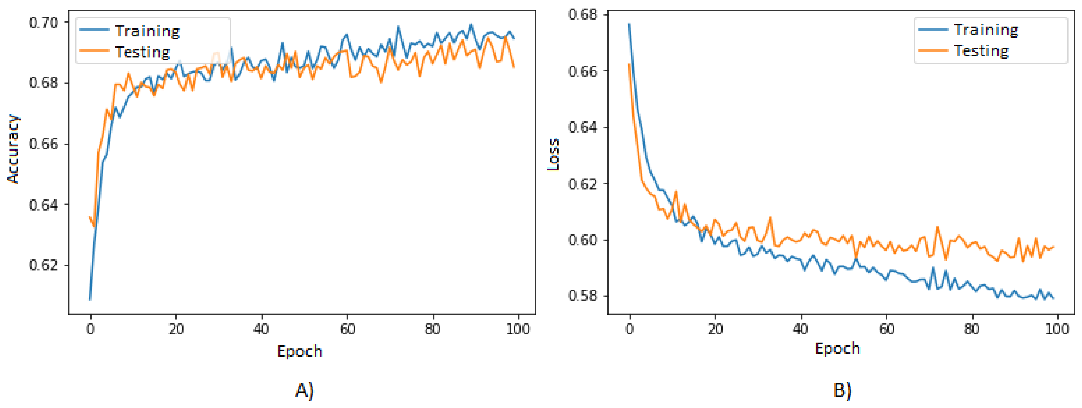
| Epochs | Accuracy | Loss Function | Processing Time (s) |
|---|---|---|---|
| 10 | 0.67 | 0.60 | 10.44 |
| 30 | 0.68 | 0.60 | 32.02 |
| 50 | 0.68 | 0.59 | 55.46 |
| 80 | 0.69 | 0.59 | 93.57 |
| 100 | 0.69 | 0.58 | 124.55 |
| 150 | 0.68 | 0.60 | 188.21 |
| 200 | 0.68 | 0.61 | 246.74 |
| 300 | 0.69 | 0.62 | 369.06 |
| 500 | 0.70 | 0.62 | 646.86 |
| 1000 | 0.70 | 0.66 | 4152.96 |
| Layers Dense/Dropout | Neurons | Accuracy | Loss Function | Processing Time (s) |
|---|---|---|---|---|
| 2/1 | 104>0.50>2 | 0.68 | 0.60 | 36.84 |
| 3/1 | 104>0.50>1000>2 | 0.68 | 0.59 | 71.10 |
| 3/2 | 104>0.25>1000>0.50>2 | 0.69 | 0.61 | 93.86 |
| 4/1 | 104>1000>0.50>100>2 | 0.68 | 0.73 | 117.63 |
| 4/2 | 104>0.50>1000>0.50>100>2 | 0.68 | 0.59 | 119.77 |
| 4/3 | 104>0.50>1000>0.25>100>0.50/2 | 0.69 | 0.58 | 124.55 |
| 5/1 | 104>100>1000>0.50>100>2 | 0.68 | 0.91 | 129.53 |
| 5/2 | 104>100>0.50>1000>0.25>100>2 | 0.68 | 0.65 | 131.66 |
| 5/3 | 104>100>0.50>1000>0.25>100>0.50>2 | 0.69 | 0.64 | 139.37 |
| 5/4 | 104>0.25>100>0.50>1000>0.25>100>0.50>2 | 0.68 | 0.59 | 138.38 |
© 2018 by the authors. Licensee MDPI, Basel, Switzerland. This article is an open access article distributed under the terms and conditions of the Creative Commons Attribution (CC BY) license (http://creativecommons.org/licenses/by/4.0/).
Share and Cite
Zanella-Calzada, L.A.; Galván-Tejada, C.E.; Chávez-Lamas, N.M.; Rivas-Gutierrez, J.; Magallanes-Quintanar, R.; Celaya-Padilla, J.M.; Galván-Tejada, J.I.; Gamboa-Rosales, H. Deep Artificial Neural Networks for the Diagnostic of Caries Using Socioeconomic and Nutritional Features as Determinants: Data from NHANES 2013–2014. Bioengineering 2018, 5, 47. https://doi.org/10.3390/bioengineering5020047
Zanella-Calzada LA, Galván-Tejada CE, Chávez-Lamas NM, Rivas-Gutierrez J, Magallanes-Quintanar R, Celaya-Padilla JM, Galván-Tejada JI, Gamboa-Rosales H. Deep Artificial Neural Networks for the Diagnostic of Caries Using Socioeconomic and Nutritional Features as Determinants: Data from NHANES 2013–2014. Bioengineering. 2018; 5(2):47. https://doi.org/10.3390/bioengineering5020047
Chicago/Turabian StyleZanella-Calzada, Laura A., Carlos E. Galván-Tejada, Nubia M. Chávez-Lamas, Jesús Rivas-Gutierrez, Rafael Magallanes-Quintanar, Jose M. Celaya-Padilla, Jorge I. Galván-Tejada, and Hamurabi Gamboa-Rosales. 2018. "Deep Artificial Neural Networks for the Diagnostic of Caries Using Socioeconomic and Nutritional Features as Determinants: Data from NHANES 2013–2014" Bioengineering 5, no. 2: 47. https://doi.org/10.3390/bioengineering5020047
APA StyleZanella-Calzada, L. A., Galván-Tejada, C. E., Chávez-Lamas, N. M., Rivas-Gutierrez, J., Magallanes-Quintanar, R., Celaya-Padilla, J. M., Galván-Tejada, J. I., & Gamboa-Rosales, H. (2018). Deep Artificial Neural Networks for the Diagnostic of Caries Using Socioeconomic and Nutritional Features as Determinants: Data from NHANES 2013–2014. Bioengineering, 5(2), 47. https://doi.org/10.3390/bioengineering5020047