
Technical Guidelines to Extract and Analyze VGI from Different Platforms


Abstract
:1. Introduction
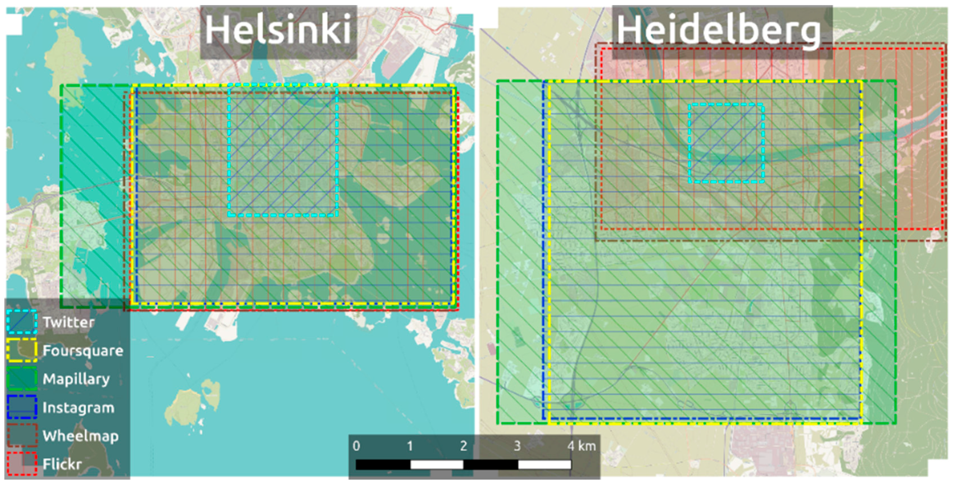
2. Data Description
3. Material and Methods
3.1. Software Requirements
3.2. Interacting with APIs
3.2.1. Making Requests in a Python Environment
3.2.2. API Methods
3.3. Exporting Data from APIs
3.3.1. Plain CSV
3.3.2. GeoJSON
3.3.3. Shapefile
3.3.4. PostGIS
3.4. Extracting Summary Statistics in an R Environment
3.4.1. Data Access
3.4.2. Data Exploration and Analysis
4. Case Studies
5. Discussion
Supplementary Materials
Author Contributions
Conflicts of Interest
Appendix A. Acquiring a User Access_Token and Token_Secret for Authenticated Twitter Requests
import tweepy

consumer_token = “Your apps token”
consumer_secret = “Your apps secret”

def get_user_tokens(consumer_token, consumer_secret):
    auth = tweepy.OAuthHandler(consumer_token, consumer_secret)
    print “Navigate to the following web page and authorize your application”
    print(auth.get_authorization_url())
    pin = raw_input(“Enter the PIN acquired on Twitter website”).strip()
    token = auth.get_access_token(verifier=pin)
    access_token = token[0]
    token_secret = token[1]
    print “With the following tokens, your application should be able to make requests on behalf of the specific user”
    print “Access token: %s” % access_token
    print “Token secret: %s” % token_secret
    return access_token, token_secret

access_token, token_secret = get_user_tokens(consumer_token, consumer_secret)
Appendix B. Searching for Tweets within a Given Radius around a Center Point Using an Existing API Wrapper
import tweepy

# Set your credentials as explained in the Authentication section
consumer_key = “Your consumer key”
consumer_secret = “Your consumer secret”
# Access tokens are needed only for operations that require authenticated requests
access_key = “Authorized access token acquired from a user”
access_secret = “Authorized access token secret”

# Set up your client
auth = tweepy.OAuthHandler(consumer_key, consumer_secret)
auth.set_access_token(access_key, access_secret)
api = tweepy.API(auth)

# Get some tweets around a center point (see http://docs.tweepy.org/en/v3.5.0/api.html#API.search)
tweets = api.search(geocode=‘37.781157,-122.398720,1km’)

# Print all tweets
for tweet in tweets:
    print “%s said: %s at %s. Location: %s” % (tweet.user.screen_name, tweet.text, tweet.created_at, tweet.geo[‘coordinates’])
    print “---”
Appendix C. Accessing Wheelmap API through Direct HTTP Requests in Python
import json
import urllib2

api_key = ‘xxx’

class WheelmapItem:
    def __init__(self, name, osm_id, lat, lon, category, node_type, accessible):
        self.name = name
        self.osm_id = osm_id
        self.lat = lat
        self.lon = lon
        self.category = category
        self.node_type = node_type
        self.accessible = accessible

    def getName(self):
        if not self.name:
            return “
        else:
            return self.name.encode(‘utf-8’)

def getWheelmapNodes(ll_lat, ll_lon, ur_lat, ur_lon, page, accessible):
    bbox = str(ll_lat) + ‘,’ + str(ll_lon) + ‘,’ + str(ur_lat) + ‘,’ + str(ur_lon)
    url = ‘http://wheelmap.org/api/nodes?api_key=‘ + api_key + ‘&bbox=‘ + bbox + ‘&page=‘ + str(page)
    if accessible != None:
    	url = url + ‘&wheelchair=‘ + accessible
    headers = {‘User-Agent’:’Python’}

    req = urllib2.Request(url, None, headers)

    print (url)
    resp = urllib2.urlopen(req).read().decode(‘utf-8’)
    return json.loads(resp)

# When we get the first load of data we can read the meta info to see how many pages there are in total

firstPage = getWheelmapNodes(8.638939,49.397075,8.727843,49.429415,1,None)
numPages = firstPage[‘meta’][‘num_pages’]

# so now we need to loop through each page and store the info
pagedData = []
pagedData.append(firstPage)

for i in range (2,numPages+1):
    pagedData.append(getWheelmapNodes(8.638939,49.397075,8.727843,49.429415,i,None))

# now that we have the data we should go through and create a list of items
# for now we will store the name, location, category, node type, accessibility and osm id
items = []
for i in range (0,len(pagedData)):
    page = pagedData[i]
    # go through each item
    nodes = page[‘nodes’]
    for node in nodes:
        item = WheelmapItem(node[‘name’], node[‘id’], node[‘lat’], node[‘lon’], node[‘category’][‘identifier’], node[‘node_type’][‘identifier’], node[‘wheelchair’])
        items.append(item)

print(‘Total items read: ‘ + str(len(items)))
Appendix D. Writing Result Tweets as a CSV File
import tweepy
import csv

# Set your credentials as explained in the Authentication section
consumer_key = “Your consumer key”
consumer_secret = “Your consumer secret”
# Access tokens are needed only for operations that require authenticated requests
access_key = “Authorized access token acquired from a user”
access_secret = “Authorized access token secret”

# Set up your client
auth = tweepy.OAuthHandler(consumer_key, consumer_secret)
auth.set_access_token(access_key, access_secret)
api = tweepy.API(auth)

# Get some tweets around a center point (see http://docs.tweepy.org/en/v3.5.0/api.html#API.search)
tweets = api.search(geocode=‘60.1694461,24.9527073,1km’)

data = {
    “username”: ““,
    “tweet_id”: ““,
    “text”: ““,
    “created_at”: ““,
    “lat”: ““,
    “lon”: ““
}
# Init a CSV writer
with open(“tweet_export.csv”, “wb”) as csvfile:
    fieldnames = [“username”, “tweet_id”, “text”, “created_at”, “lat”, “lon”]
    writer = csv.DictWriter(csvfile, delimiter=‘,’, quotechar=‘“‘, quoting = csv.QUOTE_MINIMAL, fieldnames=fieldnames)
    writer.writeheader()
# Loop through all tweets in the result set and write specific fields in the CSV
    for tweet in tweets:
        try:
            data[“username”] = tweet.user.screen_name
            data[“tweet_id”] = tweet.id
            data[“text”] = tweet.text.encode(‘utf-8’)
            data[“created_at”] = str(tweet.created_at)
            data[“lon”] = tweet.geo[‘coordinates’][0]
            data[“lat”] = tweet.geo[‘coordinates’][1]
            writer.writerow(data)
        except:
            print ‘Error occured. Field does not exist.’
Appendix E. Function to Extend Appendix C with GeoJSON Export
# This method takes a list of WhelmapItems and writes them to a GeoJSON file

def exportWheelmapNodes(node_list, file_name):
# Init geojson object
    geojson = {
        “type”: “FeatureCollection”,
        “features”: []
    }

    # Loop through the list and append each feature to the GeoJSON
    for node in node_list:
        # Populate feature skeleton
        feature = {
            “type”: “Feature”,
            “geometry”: {
                “type”: “Point”,
                “coordinates”: [node.lon, node.lat]
            },
            “properties”: {
                “name”: node.getName(),
                “osm_id”: node.osm_id,
                “category”: node.category,
                “node_type”: node.node_type,
                “accessible”: node.accessible
            }
        }
        # Append WheelnodeItem to GeoJSON features list
        geojson[“features”].append(feature)

    # Finally write the output geojson file
    f = open(file_name, “w”)
    f.write(json.dumps(geojson))
    f.close()

# Use it as:
exportWheelmapNodes(items, “wheelmap_nodes.geojson”)
Appendix F. Writing Mapillary Image Dataset to a Shapefile
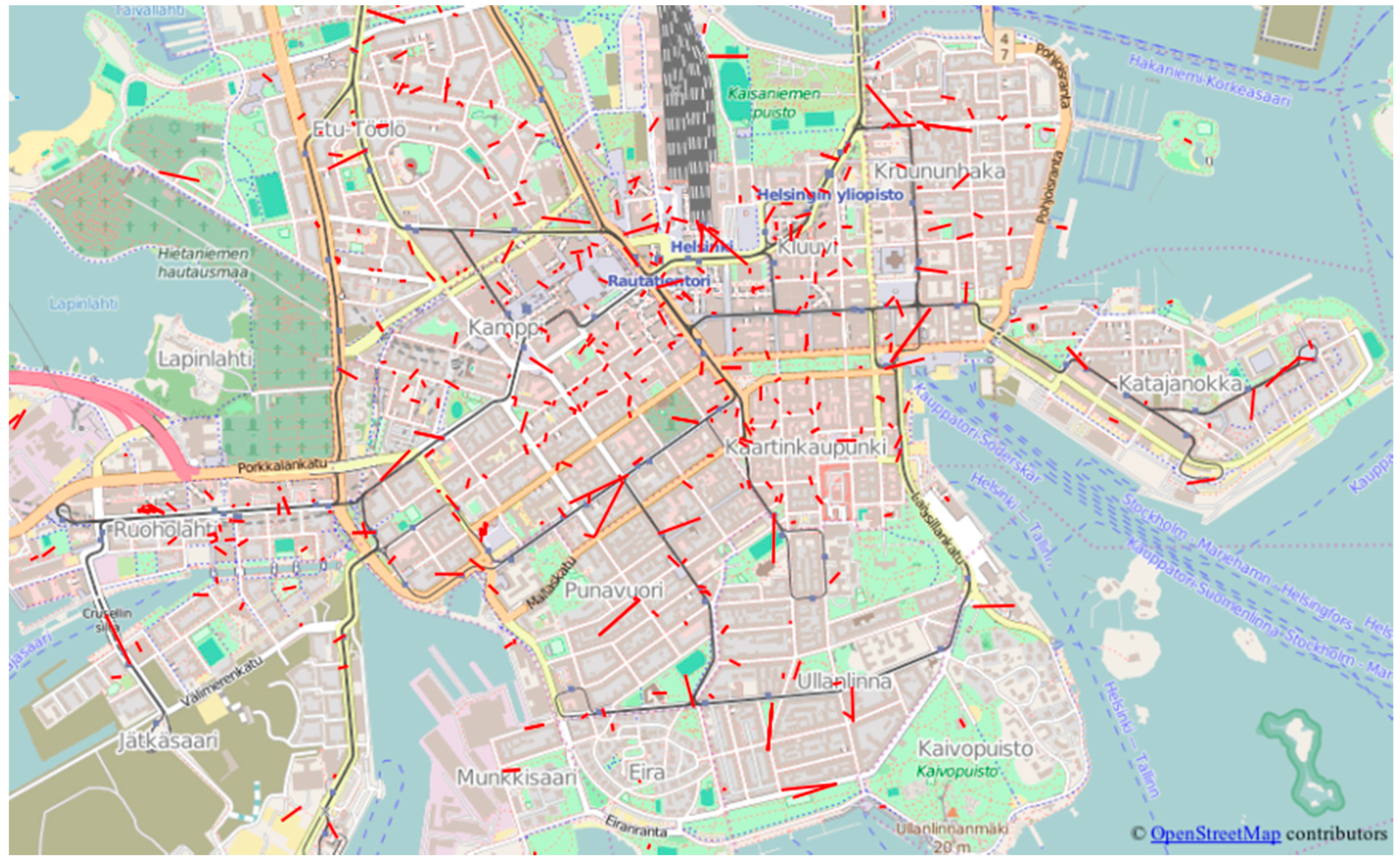
import requests
import json
import shapefile
from datetime import datetime

mapillary_api_url = “https://a.mapillary.com/v2/“
api_endpoint = “search/im”
client_id = “Your Mapillary Client ID”

request_params = {
    “client_id”: client_id,
    “min_lat”: 60.1693326154,
    “max_lat”: 60.17107241,
    “min_lon”: 24.9497365952,
    “max_lon”: 24.9553370476,
    “limit”: 100
}

# Make a GET requests
photos = requests.get(mapillary_api_url + api_endpoint + ‘?client_id=‘ + client_id + ‘&min_lat=60.1693326154&max_lat=60.17107241&min_lon=24.9497365952&max_lon=24.9553370476’)
photos = json.loads(photos.text)

# Init shapefile
writer = shapefile.Writer(shapefile.POINT)
writer.autoBalance = 1
writer.field(‘image_url’, ‘C’)
writer.field(‘captured_at’, ‘C’)
writer.field(‘username’, ‘C’)
writer.field(‘camera_angle’, ‘C’)

# Add each photo to shapefile
for photo in photos:
    writer.point(photo[‘lon’], photo[‘lat’])
    writer.record(image_url=‘http://mapillary.com/map/im/‘ + photo[‘key’], username=photo[‘user’], camera_angle=str(photo[‘ca’]), captured_at=str(datetime.fromtimestamp(photo[‘captured_at’]/1000)))
writer.save(‘my_mapillary_photos.shp’)
file = open(filename + ‘.prj’, ‘w’)
# Manually add projection file
file.write(‘GEOGCS[“GCS_WGS_1984”,DATUM[“D_WGS_1984”,SPHEROID[“WGS_1984”,6378137,298.257223563]],PRIMEM[“Greenwich”,0],UNIT[“Degree”,0.017453292519943295]]’)
file.close()
Appendix G. Setting up a PostgreSQL Database before Inserting OSM Data from OverpassAPI (SQL Statements)
-- Add PostGIS extension
CREATE EXTENSION postgis;
-- Add hstore extension to store tags as key-value pairs
CREATE EXTENSION hstore;
-- Init table
CREATE TABLE drinking_water (
  id bigint,
   user varchar,
   user_id int,
   created_at timestamp,
   version int,
   changeset int,
   tags hstore
);
-- Add a POINT geometry column to the table
SELECT AddGeometryColumn(‘drinking_water’, ‘geom’, 4326, ‘POINT’, 2);
Appendix H. Populating a PostgreSQL Table with OSM Data from OverpassAPI
import psycopg2
import json
import requests

# This function calls OverpassAPI and asks for all nodes that contain “amenity”->“drinking_water” tag
def query_nodes(bbox):
    # OverpassAPI url
    overpassAPI = ‘http://overpass-api.de/api/interpreter‘

    postdata = “‘
        [out:json][bbox:%s][timeout:120];
        (
        node[“amenity” = “drinking_water”]
        );
        out geom;
        out meta;
        >;
        “‘
    # Sending HTTP request toward OverpassAPI
    data = requests.post(overpassAPI, postdata % (bbox))
    # Parse response
    data = json.loads(data.text)
    return data

# This function uploads the data to the PostgreSQL server
def upload_data(data):
    with_no_geom = 0
    sql = ‘INSERT INTO drinking_water (id, user, user_id, created_at, version, changeset, tags, geom)
VALUES (%s, %s, %s, %s, %s, %s, ST_SetSRID(ST_MakePoint(%s, %s), 4326));’

    # Define a connection
    conn = psycopg2.connect(host = ‘localhost’, user = ‘postgres’, password=‘postgres’, dbname = ‘osm_data’)
    psycopg2.extras.register_hstore(conn)
    # Initialize a cursor
    cursor = conn.cursor()
    # Loop through all OSM nodes
    for node in data[‘elements’]:
        # Call the INSERT INTO sql statement with data from the current node
        cursor.execute(sql,(node[‘id’], node[‘user’], node[‘uid’], node[‘timestamp’], node[‘version’], node[‘changeset’], node[‘lon’], node[‘lat’]))
    # Finally commit all changes in the database
    conn.commit()

# Lago Maggiore
bbox = ‘45.698507, 8.44299,46.198844,8.915405’

# Start with putting all nodes in the variable called drinking_water
drinking_water = query_nodes(bbox)
# Pass this variable containing all OSM nodes to the upload script that will insert it to the PostgreSQL database
upload_data(drinking_water)


# Alternatively you can visualize your data in QGIS, or you can simply make a query toward the
# database to see if it worked

# -- Select 10 nodes
# SELECT id, user, created_at, tags from drinking_water limit 10
Appendix I. Reading Csv Files in a Statistical Environment (Rscript)
locations <- read.csv(‘locations.csv’, as.is=T, quote=“”“)
photos <- read.csv(‘photos.csv’, as.is=T, quote=“”“)
# No quoting in this file. Always check source first!
hashtags <- read.csv(‘hashtags.csv’, as.is=T, header=F)
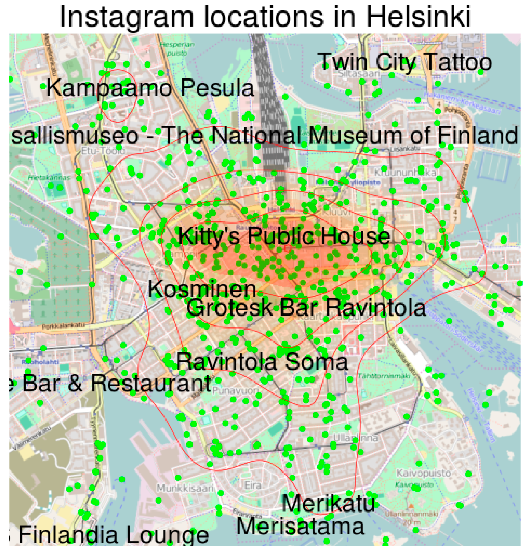
Appendix J. Visualizing Instagram Locations (Rscript)
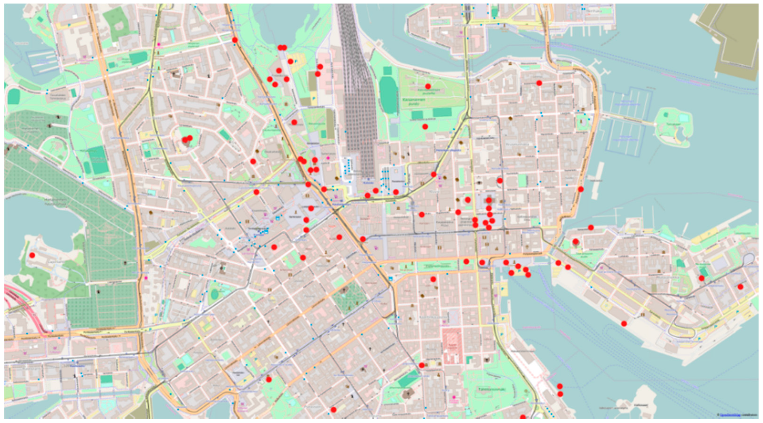
library(‘ggplot2’)
library(‘plyr’)
library(‘wordcloud’)
library(‘ggmap’)
# Once the packages are loaded, continue with the creation of a map of locations.

# Set map center to the arithmetic mean of lat-long coordinates
center <- c(lon = mean(locations$lon), lat = mean(locations$lat))
# Init map background to OpenStreetMap tiles at zoom level 15
background <- get_map(location = center, source = ‘osm’, zoom = 15)

# Create a ggmap object
map <- ggmap(background, extent = ‘device’)

# Hint: typing map to the console (calling your object) will print out the background map

# Populate map plot with points using the geom_point() function
map <- map + geom_point(data = locations, aes(x = lon, y = lat), color = ‘green’, size = 2)

# Heatmap style visualization of density with countour lines
map <- map + stat_density2d(data=locations, aes(x = lon,y = lat, fill = ..level.., alpha = ..level..), geom=‘polygon’, size = .3) +
scale_fill_gradient(low = ‘yellow’, high = ‘red’, guide = F) +
stat_density2d(data = locations, aes(x = lon, y = lat), bins = 5, color = ‘red’, size = .3) +
scale_alpha(range = c(0, .2), guide = F)

# Finally, we can annotate our plot

map <- map + ggtitle(‘Instagram locations in Helsinki’) + geom_text(data = locations[sample(1:nrow(locations),20),], aes(x = lon, y = lat, label = name), size = 5, check_overlap=T)

# Type “map” to the console again to see your final map.
Appendix K. Simple Data Exploration (Rscript)
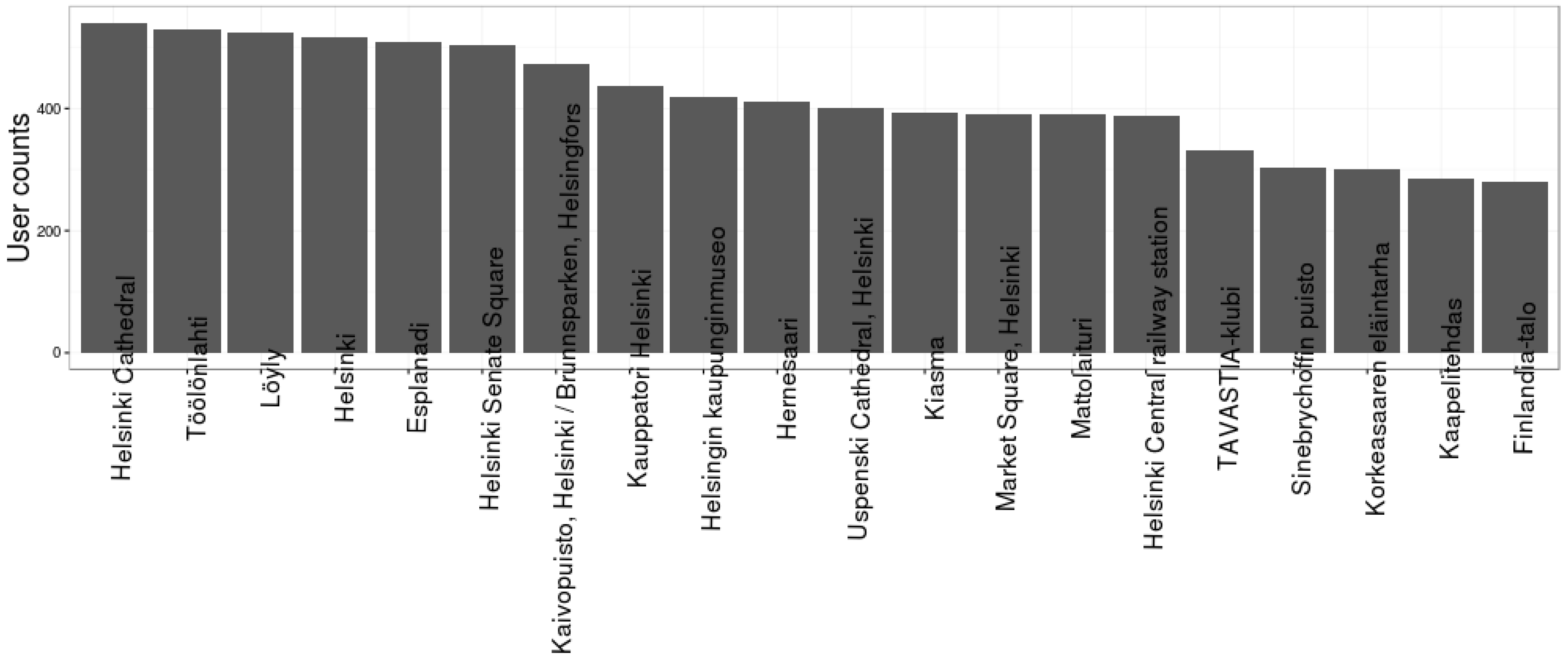
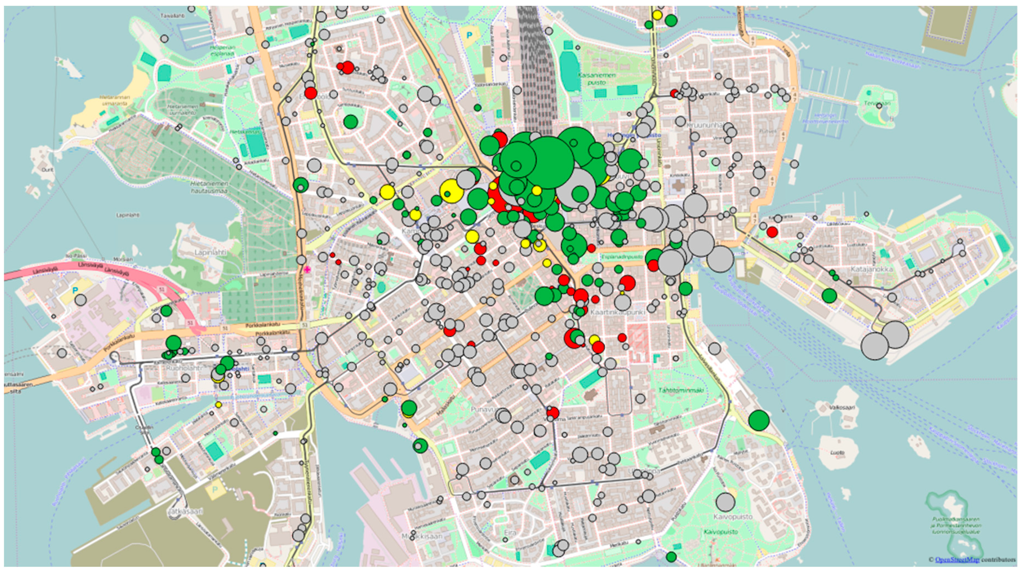
# Total number of photos
nrow(photos)

# Total number of unique users posting photos in these locations
length(unique(photos$username))

# Summarizing data by location
# Check out also count(), join() and merge() functions!
locations[‘user_count’] <- NA
locations[‘photo_count’] <- NA
# sapply() summarizes users by applying the length() function for all location_ids (i.e., what is the
# length of the list of users for a location?)
locations[‘user_count’] <- sapply(locations$id, function(x)
length(unique(photos[photos$location_id==x,]$username)))
# Again, we answer to the question “How many rows do we have after truncating our photos data
# frame to the specific location?” with sapply()
locations[‘photo_count’] <- sapply(locations$id, function(x) nrow(photos[photos$location_id==x,]))

# Draw histograms to see how popularity of places is distributed

# Histogram of user counts by location
hist(locations$user_count)
# Histogram of uploaded photos for each location
hist(locations$photo_count)

# Extract top 20 places with most users
plot_data <- locations[order(-locations$user_count),][1:20,]
plot_data <- transform(plot_data[,c(‘name’,’user_count’)], name = reorder(name, order(user_count, decreasing=T)))

# Create a bar plot of user counts for the 20 most visited locations
ggplot(plot_data, aes(x = name, y = user_count)) + geom_bar(stat = ‘identity’) + theme_bw() + theme(axis.text.x = element_text(angle = 90), axis.title.x = element_blank()) + ylab(‘User counts’)
Appendix L. Exploring Instagram Photo Upload Intensity over the Days of Week (Rscript)
# Extract the Day of Week from the timestamp
days <- format(as.Date(photos$created_at), format = ‘%A’)

# Calculate frequencies using the count() function from the plyr package
freq_table <- count(days)

ggplot(freq_table, aes(x = x, y = freq)) + geom_bar(stat = ‘identity’) + theme_bw() + xlab(‘Day of week’) + ylab(‘Photos uploaded’)
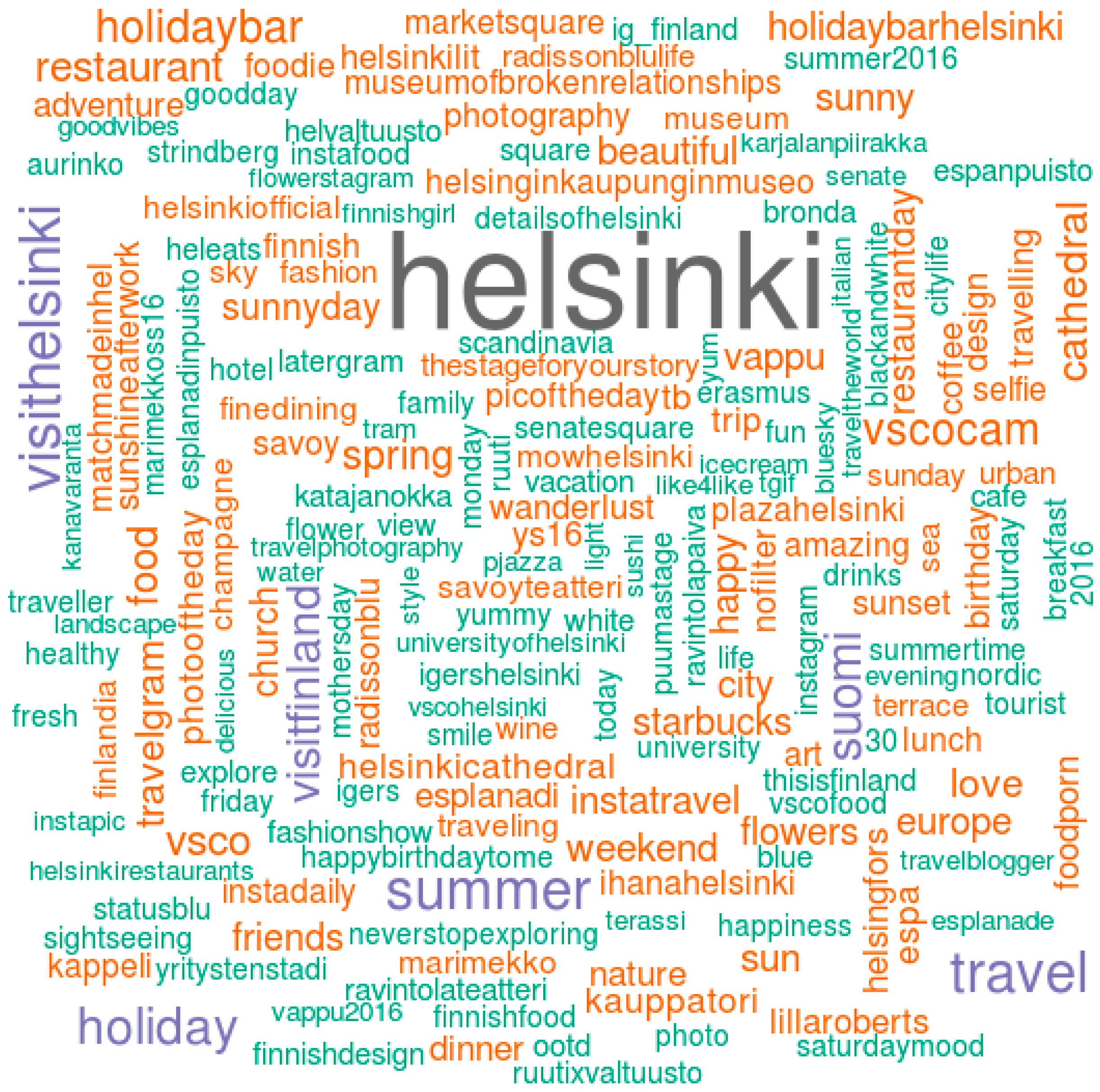
Appendix M. Generating a Wordcloud of Instagram Hashtags (Rscript)
# Let’s count the occurances of each hashtag with the count() function
hashtag_freq <- count(hashtags)

# We can also rename the columns
names(hashtag_freq) <- c(“hashtag”,”freq”)

# Finally, let’s generate a wordcloud.
wordcloud(words = hashtag_freq$hashtag, freq = sqrt(hashtag_freq$freq), min.freq = 1, max.words=200, rot.per = 0.25,colors = brewer.pal(8,”Dark2”))

# Hint: type ?wordcloud in the console if you’re using RStudio to see what additional parameters you can use to control the appearance of your wordcloud.
Appendix N. Fitting a Linear Regression on Instagram “likes” and Number of Tagged Users (Rscript)
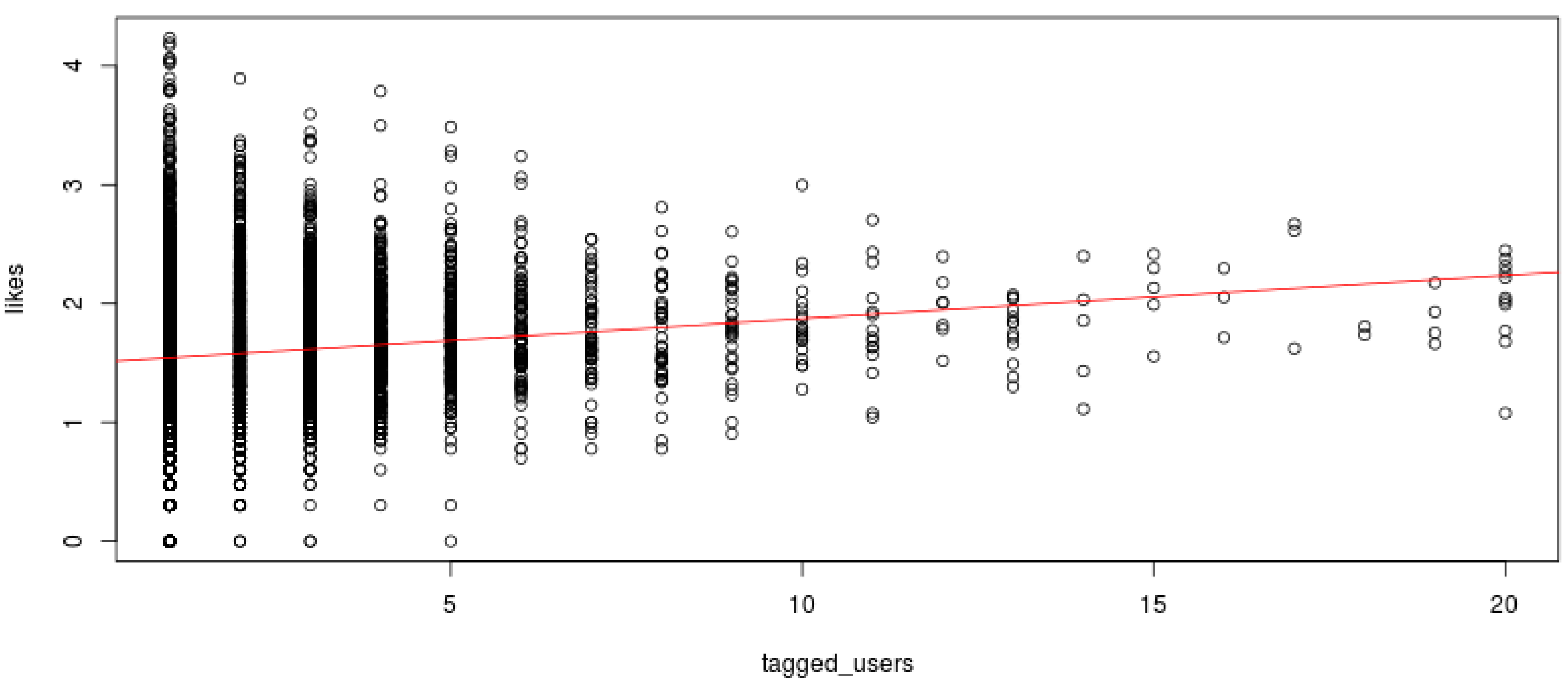
# Let’s drop those photos with 0 tagged users and 0 likes
subset <- photos[photos$tagged_users > 0 & photos$likes > 0,]

# Since we’re about to build a linear regression model, let’s do a dummy normality check
hist(subset$likes)

# Log transform like counts since they’re not normally distributed
likes <- log10(subset$likes)
tagged_users <- subset$tagged_users

# Build simple linear regression
reg <- lm(likes ~ tagged_users)
plot(tagged_users, likes)
abline(reg, col = ‘red’)
# Check the summary to see if the relationship is statistically significant
summary(reg)
References
- Krumm, J.; Davies, N.; Narayanaswami, C. User-generated content. IEEE Pervasive Comput. 2008, 4, 10–11. [Google Scholar] [CrossRef]
- Sester, M.; Arsanjani, J.J.; Klammer, R.; Burghardt, D.; Haunert, J.-H. Integrating and Generalising Volunteered Geographic Information. In Abstracting Geographic Information in a Data Rich World; Springer: Cham, Switzerland, 2014; pp. 119–155. [Google Scholar]
- Hecht, B.; Hong, L.; Suh, B.; Chi, E.H. Tweets from justin bieber’s heart: The dynamics of the location field in user profiles. In Proceedings of the SIGCHI Conference on Human Factors in Computing Systems, Vancouver, BC, Canada, 7–12 May 2011; pp. 237–246.
- Flatow, D.; Naaman, M.; Xie, K.E.; Volkovich, Y.; Kanza, Y. On the accuracy of hyper-local geotagging of social media content. In Proceedings of the Eighth ACM International Conference on Web Search and Data Mining, Shanghai, China, 2–6 February 2015; pp. 127–136.
- Haklay, M. Citizen Science and Volunteered Geographic Information: Overview and Typology of Participation. In Crowdsourcing Geographic Knowledge; Sui, D., Elwood, S., Goodchild, M., Eds.; Springer: Berlin, Germany, 2013; pp. 105–122. [Google Scholar]
- Girres, J.F.; Touya, G. Quality assessment of the french openstreetmap dataset. Trans. GIS 2010, 14, 435–459. [Google Scholar] [CrossRef]
- Haklay, M. How good is volunteered geographical information? A comparative study of openstreetmap and ordnance survey datasets. Environ. Plan. B Plan. Des. 2010, 37, 682–703. [Google Scholar] [CrossRef]
- Juhász, L.; Hochmair, H.H. User contribution patterns and completeness evaluation of Mapillary, a crowdsourced street level photo service. Trans. GIS 2016. [Google Scholar] [CrossRef]
- Mooney, P.; Corcoran, P.; Winstanley, A. A study of data representation of natural features in openstreetmap. In Proceedings of the 6th GIScience 2010 International Conference, Zurich, Switzerland, 14–17 September 2010; pp. 150–156.
- Goodchild, M.F. Citizens as voluntary sensors: Spatial data infrastructure in the world of web 2.0 (editorial). Int. J. Spat. Data Infrastruct. Res. 2007, 2, 24–32. [Google Scholar]
- Arsanjani, J.J.; Zipf, A.; Mooney, P.; Helbich, M. An Introduction to Openstreetmap in Geographic Information Science: Experiences, Research, and Applications. In Openstreetmap in Giscience; Springer: Cham, Switzerland, 2015; pp. 1–15. [Google Scholar]
- Juhász, L.; Hochmair, H.H. Cross-Linkage between Mapillary Street Level Photos and OSM edits. In Geospatial Data in a Changing World; Springer: Cham, Switzerland, 2016; pp. 141–156. [Google Scholar]
- Antoniou, V.; Morley, J.; Haklay, M. Web 2.0 geotagged photos: Assessing the spatial dimension of the phenomenon. Geomatica 2010, 64, 99–110. [Google Scholar]
- Spinsanti, L.; Ostermann, F. Automated geographic context analysis for volunteered information. Appl. Geogr. 2013, 43, 36–44. [Google Scholar] [CrossRef]
- Schade, S.; Díaz, L.; Ostermann, F.; Spinsanti, L.; Luraschi, G.; Cox, S.; Nuñez, M.; Longueville, B.D. Citizen-based sensing of crisis events: Sensor web enablement for volunteered geographic information. Appl. Geomat. 2013, 5, 3–18. [Google Scholar] [CrossRef]
- Lingad, J.; Karimi, S.; Yin, J. Location extraction from disaster-related microblogs. In Proceedings of the 22nd International Conference on World Wide Web, Rio de Janeiro, Brazil, 13–17 May 2013; pp. 1017–1020.
- Kinsella, S.; Murdock, V.; O’Hare, N. I’m eating a sandwich in glasgow: Modeling locations with tweets. In Proceedings of the 3rd International Workshop on Search And Mining User-Generated Contents, Glasgow, UK, 24–28 October 2011; pp. 61–68.
- Gelernter, J.; Mushegian, N. Geo-parsing messages from microtext. Trans. GIS 2011, 15, 753–773. [Google Scholar] [CrossRef]
- Intagorn, S.; Lerman, K. Placing user-generated content on the map with confidence. In Proceedings of the 22nd ACM SIGSPATIAL International Conference on Advances in Geographic Information Systems, Dallas, TX, USA, 4–7 November 2014; pp. 413–416.
- Sample Datasets. Available online: https://github.com/jlevente/link-vgi/tree/master/sample_datasets (accessed on 20 September 2016).
- Laakso, M.; Sarjakoski, T.; Sarjakoski, L.T. Improving accessibility information in pedestrian maps and databases. Cartographica 2011, 46, 101–108. [Google Scholar] [CrossRef]
- Antoniou, V.; Fonte, C.C.; See, L.; Estima, J.; Arsanjani, J.J.; Lupia, F.; Minghini, M.; Foody, G.; Fritz, S. Investigating the feasibility of geo-tagged photographs as sources of land cover input data. ISPRS Int. J. Geo-Inf. 2016, 5, 64. [Google Scholar] [CrossRef]
- Kahle, D.; Wickham, H. Ggmap: Spatial visualization with ggplot2. R J. 2013, 5, 144–161. [Google Scholar]
- Ayala, G.; Epifanio, I.; Simó, A.; Zapater, V. Clustering of spatial point patterns. Comput. Stat. Data Anal. 2006, 50, 1016–1032. [Google Scholar] [CrossRef]
- Goodchild, M.F.; Glennon, J.A. Crowdsourcing geographic information for disaster response: A research frontier. Int. J. Digit. Earth 2010, 3, 231–241. [Google Scholar] [CrossRef]
- Flanagin, A.J.; Metzger, M.J. The credibility of volunteered geographic information. GeoJournal 2008, 72, 137–148. [Google Scholar] [CrossRef]
- Scassa, T. Legal issues with volunteered geographic information. Can. Geogr. 2013, 57, 1–10. [Google Scholar] [CrossRef]


| Data Source—API Method | Attributes | Data Volume * | File Names |
|---|---|---|---|
| Flickr photos.search (https://www.flickr.com/services/api/flickr.photos.search.html) | “photo_id”, “url”, “lat”, “lon” | 1850 + 625 | flickr_[city].csv |
| Foursquare **—/venues/search (https://developer.foursquare.com/docs/venues/search)/venues (https://developer.foursquare.com/docs/venues/venues) | Venues: “id”, “name”, “tipcount”, “checkincount”, “usercount”, “url”, “photo_count”, “tags”, “lat”, “lon” Photos: “photo_id”, “source”, “created_at”, “photo_url”, “user_id”, ”user_name”, ”venue_id” | Venues: 5141 + 1239; Photos: 12783 + 2233 | foursquare_venue_[city].csv |
| foursquare_venue_photos_[city].csv | |||
| Instagram**—/locations/search locations/media/recent (https://www.instagram.com/developer/endpoints/locations/) | Locations: “id”, “name”, “lat”, “lng” Photos: “id”, “username”, “user_id”, “likes”, “tags”, “comment”, “text”, “users_in_photo”, “filter”, “url”, “lat”, “lon”, “photo_url”, “location_id”, ”created_at” | Locations: 819 + 286; Photos: 38427 + 7577 | instagram_locations_[city].csv |
| instagram_photos_[city].csv | |||
| Mapillary—/search/im (https://a.mapillary.com/#get-searchim) | “user”, “key”, “lon”, “lat”, “url”, “captured_at”, “ca” (camera angle) | 21078 + 14052 | mapillary_photos_[city].csv |
| Twitter—/search/tweets (https://dev.twitter.com/rest/reference/get/search/tweets) | “username”, “tweet_id”, “text”, “created_at”, “lat”, “lon” | 129 + 41 | tweets_[city].csv |
| Wheelmap—/nodes (http://wheelmap.org/en/api/docs/resources/nodes) | “osm_id”, “name”, “lat”, “lon”, “category”, “type”, “accessible” | 2180 + 2436 | wheelmap_[city].csv |
| Service | Registration Address | Instructions | Parameters Needed |
|---|---|---|---|
| Wheelmap.org | http://wheelmap.org/users/sign_in (with an OSM profile) | Once logged in, navigate to your “Edit profile page” | authentication_token |
| Flickr | Yahoo (register for Yahoo or use an existing Yahoo account) | Create a new application (https://www.flickr.com/services/apps/create/) and check “Sharing & Extending”/Your API keys” | api_key, api_secret |
| Mapillary | http://www.mapillary.com/map/signup Create a Mapillary profile | Once logged in, navigate to https://www.mapillary.com/app/settings/developers and hit Register an application. | client_id |
| Sign up for Twitter | Go to Twitter Apps (https://apps.twitter.com/app/new) and hit Create New App. Check your credentials under “Keys and Access Tokens” | api_key, api_secret |
© 2016 by the authors; licensee MDPI, Basel, Switzerland. This article is an open access article distributed under the terms and conditions of the Creative Commons Attribution (CC-BY) license (http://creativecommons.org/licenses/by/4.0/).
Share and Cite
Juhász, L.; Rousell, A.; Jokar Arsanjani, J. Technical Guidelines to Extract and Analyze VGI from Different Platforms. Data 2016, 1, 15. https://doi.org/10.3390/data1030015
Juhász L, Rousell A, Jokar Arsanjani J. Technical Guidelines to Extract and Analyze VGI from Different Platforms. Data. 2016; 1(3):15. https://doi.org/10.3390/data1030015
Chicago/Turabian StyleJuhász, Levente, Adam Rousell, and Jamal Jokar Arsanjani. 2016. "Technical Guidelines to Extract and Analyze VGI from Different Platforms" Data 1, no. 3: 15. https://doi.org/10.3390/data1030015
APA StyleJuhász, L., Rousell, A., & Jokar Arsanjani, J. (2016). Technical Guidelines to Extract and Analyze VGI from Different Platforms. Data, 1(3), 15. https://doi.org/10.3390/data1030015