Adjustable Robust Singular Value Decomposition: Design, Analysis and Application to Finance

Abstract

The Singular Value Decomposition (SVD) is a fundamental algorithm used to understand the structure of data by providing insight into the relationship between the row and column factors. SVD aims to approximate a rectangular data matrix, given some rank restriction, especially lower rank approximation. In practical data analysis, however, outliers and missing values maybe exist that restrict the performance of SVD, because SVD is a least squares method that is sensitive to errors in the data matrix. This paper proposes a robust SVD algorithm by applying an adjustable robust estimator. Through adjusting the tuning parameter in the algorithm, the method can be both robust and efficient. Moreover, a sequential robust SVD algorithm is proposed in order to decrease the computation volume in sequential and streaming data. The advantages of the proposed algorithms are proved with a financial application.

1. Introduction

The Singular Value Decomposition (SVD) of a rectangular data matrix is a powerful method in analyzing the data structure and the relationship between rows and columns. SVD has been applied in many methods, such as biplot [1], correspondence analysis [2], and principal component analysis. There are also many SVD applications, for example, image compression, gene data analysis, etc.

The SVD is a factorization of a real or complex matrix. Let $\mathbf{M}$ be a data matrix of order $m\times n$. The columns of $\mathbf{M}$ represent n attributes and its rows represent m instances.

The SVD of $\mathbf{M}$ is,

$${\mathbf{M}}_{m\times n}={\mathbf{U}}_{m\times p}{\mathbf{S}}_{p\times p}{\mathbf{V}}_{p\times n}^T$$

where $p\le min\{m,n\}, {\mathbf{U}}^T\mathbf{U}={\mathbf{V}}^T\mathbf{V}={\mathbf{I}}_p$ (${\mathbf{I}}_p$ is an identity matrix), and $\mathbf{S}=diag\{{\lambda }_1,\dots ,{\lambda }_p\},{\lambda }_1\ge \dots \ge {\lambda }_p\ge 0$.

Writing ${\mathbf{u}}_i$ and ${\mathbf{v}}_i$ for the $i^{th}$ left and right eigenvectors, respectively, and ${\lambda }_i$ for the $i^{th}$ singular-value, the SVD can be written as,

$$\mathbf{M}=\sum _{i=1}^p{\lambda }_i{\mathbf{u}}_i{\mathbf{v}}_i^T.$$

The summation of the first k ($k<p$) terms is the rank k approximation to $\mathbf{M}$.

1.1. Alternating Approach

The conventional approach of calculating the SVD through a principal component analysis of ${\mathbf{M}}^T\mathbf{M}$ and ${\mathbf{MM}}^T$ requires the data matrix to be complete, which means that it cannot be performed for the data matrix with missing elements. An alternative iterative approach introduced by Gabriel and Zamir [3] addresses this problem.

This approach is an alternating least square (ALS) algorithm that works iteratively and starts with the leading eigentriple ${\lambda }_1$, ${\mathbf{u}}_1$, and ${\mathbf{v}}_1$. It starts with an initial guess of ${\mathbf{u}}_1$. Then a least square regression is applied to every column of $\mathbf{M}$ by using ${\mathbf{u}}_1$ to get ${\lambda }_1{\mathbf{v}}_1$. At the end of the regression cycle of columns, scaling the vector estimate to unit length can give ${\mathbf{v}}_1$, and the scale factor is ${\lambda }_1$. After getting the estimation of ${\mathbf{v}}_1$, the least square regression of every row of $\mathbf{M}$ is performed by using ${\mathbf{v}}_1$ to refine ${\mathbf{u}}_1$. Then, the estimation is normalized to get the new ${\mathbf{u}}_1$. These steps are repeated until convergence. Until now, the estimation of the first eigentriple was achieved. After that, replace $\mathbf{M}$ by $\mathbf{M}-{\lambda }_1{\mathbf{u}}_1{\mathbf{v}}_1$, and start a new iteration to get the second eigentriple ${\lambda }_2$, ${\mathbf{u}}_2$, and ${\mathbf{v}}_2$.

1.2. The Effect of Noise on SVD

Since the SVD is a least squares procedure, it is highly susceptible to outliers. In practice, outliers and abnormal values in the data matrix, which can not be solved by using the ALS algorithm. In the extreme case, an individual cell can draw even the leading principal component toward itself. Conventional SVD cannot remove outliers, and the effects of noise on SVD are significant. D. Hawkins et al. introduced the AL1-SVD algorithm [4], which replaced the least square by the L1-norm. The AL1-SVD is robust to noise in some extent, but the efficiency of handling a noise free matrix is decreased. A good robust algorithm, however, should combine high robustness and high efficiency. Robustness means the algorithm can be very resistant to outliers, and efficiency means the algorithm can be very accurate in situations with less noise. The capacity of resisting noise of the AL1-SVD algorithm is fixed, which means some information were lost (inaccurately estimated) when using AL1-SVD to estimate a data matrix that has only a small portion of noise cells, or a bad estimation was made when estimating a highly contaminated matrix. Practically, the noise levels are different among different data. Therefore, a robust SVD method that can deal with most situations is needed.

This paper proposes an adjustable robust SVD algorithm, which minimize a myriad estimator, that can perform well among different noise level situations. Then, a sequential robust SVD algorithm is also proposed, which reduces the computation volume when calculating the sequential data matrix, such as financial data. The proposed algorithm is proved robust under a noise condition and efficiency under a noise free condition, which addresses the issue that the existing robust SVD algorithm cannot adapt to a different noise level condition, especially the inefficiency problem under a light noise condition. The advantages of the proposed algorithm is also shown in a financial application.

This paper begins by analyzing the robustness of different estimators including least square, L1, and myriad. Then, a discussion of the selection for the tuning parameter K of the myriad estimator is in Section 2. Section 3 illustrates the robust SVD algorithm and robust sequential SVD algorithm. In Section 4, the proposed algorithm is applied to an application in finance field.

2. Robustness Analysis

The proposed Myriad Robust SVD (MySVD) algorithm replaces the least squares norm in ALS (or L1-norm in AL1) by the myriad estimator. The myriad estimator is a robust and adjustable estimator that is resistant to outliers by adjusting its tunning parameter K. This section focuses on the analysis of robustness and efficiency for three different estimators, and also on how to select the tuning parameter K in myriad estimation.

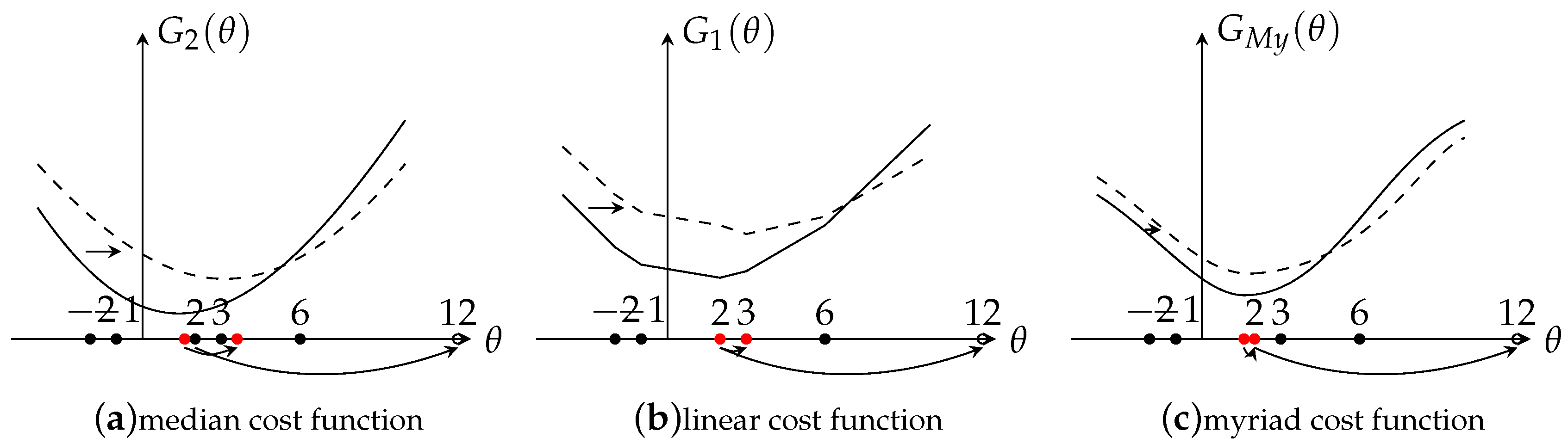
2.1. Robustness Analysis for Different Estimators

The Gaussian and Laplacian density functions lead to efficacious cost functions for the mean estimator and the median estimator as $\rho \left(x\right)=x^2$ and $\rho \left(x\right)=\left|x\right|$, respectively. The myriad estimator belongs to the M-estimator and is derived from the $\alpha$-stable distribution using the cost function $\rho \left(x\right)=log(K^2+x^2)$, where the linearity tuning parameter $K>0$ controls the impulse-resistance of the estimator (a more detailed description of K selection is given in Section 2.2). Given a set of samples $x_1,x_2,\dots ,x_N$, the cost functions and the outputs for the linear (least square or mean), median, and myriad estimators are shown in

Table 1. Cost functions and outputs for various estimators.

Estimator	Cost Function	Output, $\mathit{\theta }$
Linear	${\sum }_{i=1}^N{(x_i-\theta )}^2$	$mean\{x_1,x_2,\dots ,x_N\}$
Median	${\sum }_{i=1}^N|x_i-\theta |$	$median\{x_1,x_2,\dots ,x_N\}$
Myriad	${\sum }_{i=1}^{N}log(K^2+{(x_i-\theta )}^2)$	$myriad\{x_1,x_2,\dots ,x_N\}$

.

The linear estimator is highly sensitive to outliers; in some extreme cases, even only one sample value that is abnormal causes the final result to be dragged far away from the optimal value. The robustness of the median estimator is explained by the heavy tails of the Laplacian distribution, which makes the median estimator more resistant to outliers than the mean estimator. However, the median estimator is not robust enough in some extremely impulsive situations, especially when outliers change the samples’ order very much. Also, the median estimator is not accurate in the noise free estimation. The myriad estimator, as a tunable estimator of location derived from the theory of robust statistic, contains both robustness and efficiency. As explained in [5,6,7], the parameter K can provide the myriad estimator with a rich variety of modes of operation that range from highly resistant mode-type estimator to the very efficient class of linear estimator. The myriad estimator appears the Linear Property when $K\to \infty$. On the other hand, the myriad estimator also appears the Mode Property when $K\to 0$. The two properties, which are summarized as follows, explain the behavior of myriad estimator while tuning the parameter K.

Property 1 (Linear Property).

Given a set of samples $x_1,x_2,\dots ,x_n$, the sample myriad ${\widehat{\beta }}_K$ converges to the sample average as $K\to \infty$. This is

$$\underset{K\to \infty }{lim}{\widehat{\beta }}_K=\underset{K\to \infty }{lim}myriad\{K;x_1,\dots ,x_n\}=\frac{1}{N}\sum _{i=1}^N{x}_i$$

Property 2 (Mode Property).

Given a set of samples $x_1,x_2,\dots ,x_n$, the mode-myriad estimator, ${\widehat{\beta }}_0$ is defined as

$${\widehat{\beta }}_0=\underset{K\to 0}{lim}{\widehat{\beta }}_K,$$

The mode-myriad ${\widehat{\beta }}_0$ is always equal to one of the most repeated values in the sample. Furthermore,

$${\widehat{\beta }}_0=arg\underset{x_j\in \mathit{M}}{min}\prod _{i=1,x_i\ne x_j}^N|x_i-x_j|,$$

where M is the set of most repeated values.

Plainly, as seen in Figure 1 (the sample set is $(x_1,x_2,\dots ,x_7)=(-7,-2,\dots ,6)$, $G_{My}\left(\theta \right)$ is the myriad cost function) the larger the value of K, the closer the behavior of the myriad estimator to the linear estimator. While decreasing the value of K, the myriad moves away from the linear estimator to a more resistant estimator (in the limit case, the mode estimator, the optimal value towards the cluster $(2,2.5,3)$). These properties made the myriad estimator a very powerful estimator.

The following example illustrates the robustness and efficiency for these three estimators. Consider the observation set (noise-free) $(x_1,x_2,x_3,x_4,x_5)=(-2,3,2,-1,6)$. The output for linear estimator is ${\theta }_2={\sum }_{i=1}^5{x}_i/5=1.6$ (here, using mean square error (MSE) as an evaluation criteria, thus $1.6$ is the optimal output), for median estimator is ${\theta }_2=median\{-2,-1,2,3,6\}=2$. Since the observations are noise free, a large value of K is needed to get an accurate output, $K=20$. The output for the myriad estimator is ${\theta }_{My}={\sum }_{i=1}^{5}log({20}^2+{(x_i-\theta )}^2)=1.604$. Here, if choosing a lager K, such as $K=50$ and the output is $1.6$, the output could be more close to the optimal value $1.6$. In order to get more insights of the behavior of these estimators, a graph is drawn where the x-axis represents the output $\theta$ and y-axis represents the cost function G. Here, $G_1\left(\theta \right)={\sum }_{i=1}^N|x_i-\theta |$ denotes median cost function, $G_2\left(\theta \right)={\sum }_{i=1}^N{(x_i-\theta )}^2$ denotes linear cost function, and $G_{My}\left(\theta \right)={\sum }_{i=1}^{N}log(K^2+{(x_i-\theta )}^2)$ denotes the myriad cost function. The results are shown in Figure 2 with solid lines. Clearly, the result shows that under the noise free situation, the linear and myriad estimators could achieve the optimal output, however, the median estimator is not accurate enough.

Then, the observed data is contaminated by replacing the value 2 of $x_3$ by 12. As Figure 2 shows, the function line is shifted right from the solid line to the dashed line. With the shifting, it’s easy to find that the outputs are also shifted. For the linear estimator, the output is shifted from the optimal value $1.6$ to ${\theta }_2^{{}^{\prime }}={\sum }_{i=1}^5{x}_i/5=3.6$. The result shows that the linear estimator is very sensitive to outliers, only one abnormal value made the output very deviated from the optimal value. Compared with the linear estimator, the median estimator is more robust but the output still changed a little, from 2 to ${\theta }_2^{{}^{\prime }}=median\{-2,-1,3,6,13\}=3$. The fact is that the effect of outliers is smaller for the median estimator than the mean estimator. Besides, if the abnormal point did not change the statistic order of the data, the median estimator would not be effected. For example, replacing 3 by 12 instead of 2, the output would still be 2. However, in reality, it is highly possible that the statistic order of the data would be changed due to the random noise. Lastly, for the myriad estimator, under the noise situation, the K value needs to be changed (based on the K selection method introduced in Section 2.2) in order to fit the data and get an acceptable output. The output value of the myriad estimator is 2, which is closer to the optimal value, which shows the myriad estimator is more robust than the other two estimators. Now, based on the analysis of the properties and of the example, the conclusion can be made that the myriad is a very powerful estimator that contains both robustness and efficiency, so that it is used in the proposed robust SVD algorithm.

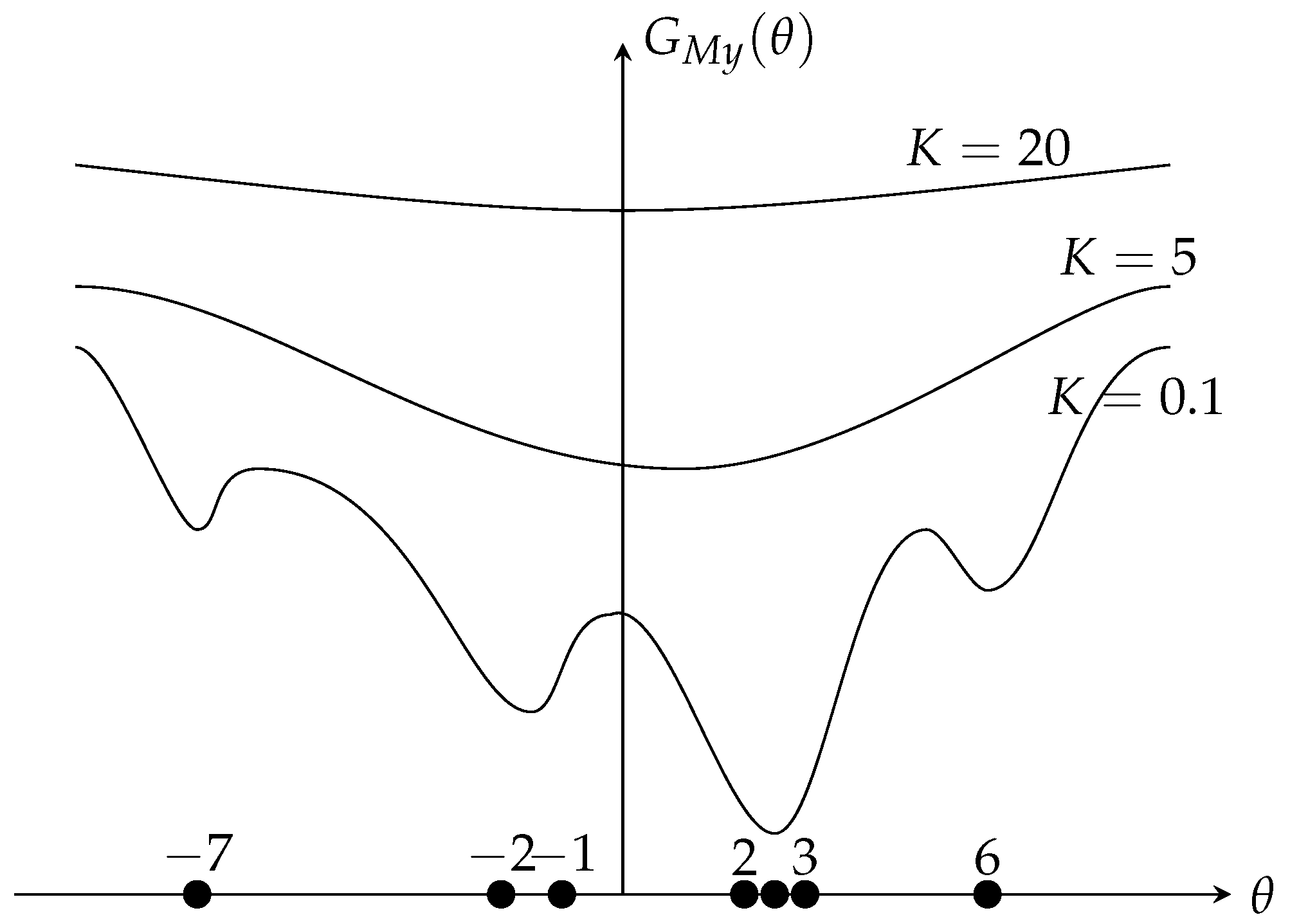
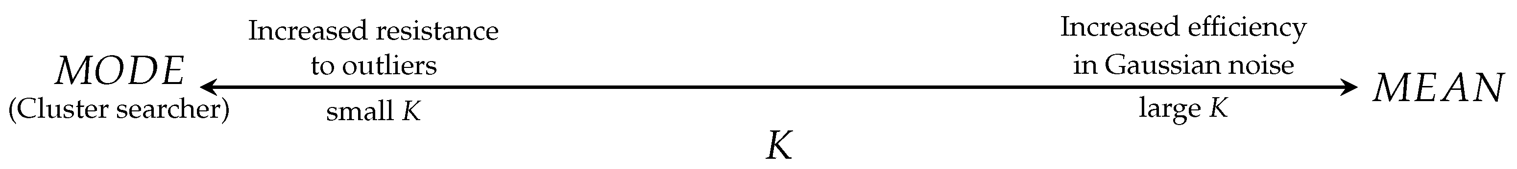
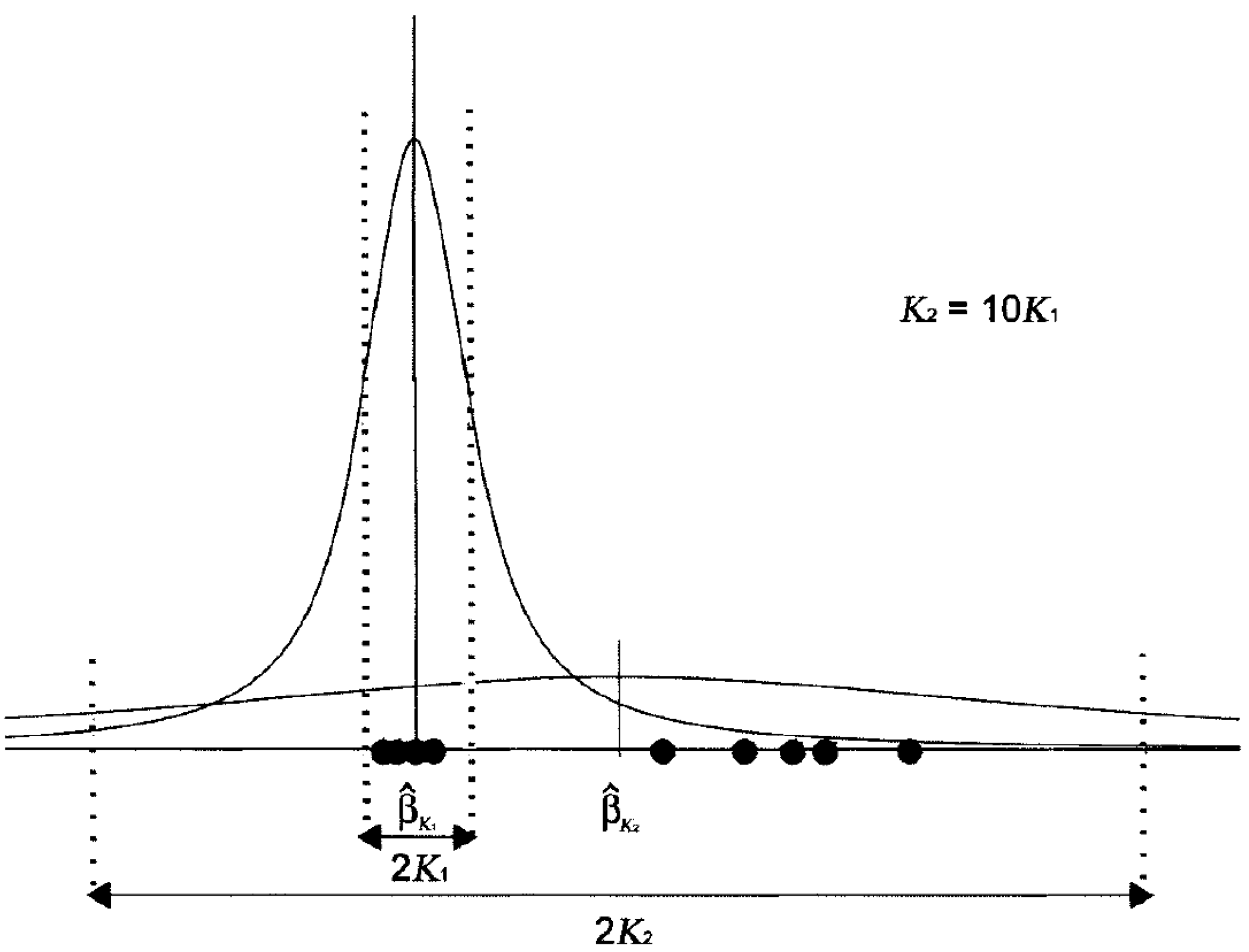
2.2. The Selection of K

The linear and mode properties indicate the behavior of the myriad estimator, which is driven by the key parameter K.

Figure 3 [5] shows how K drives the behavior of the myriad estimator. Since the myriad estimator was derived from the $\alpha$-stable distribution, the value of K is determined by the impulsiveness of noise, proposed by [8]. The noise impulsiveness is derived by estimating the stability parameter $\alpha$ [9]. There are several papers regarding the estimation of $\alpha$, such as [10,11,12]. However, in order to get an accurate $\alpha$ estimation, a large amount of samples is needed, which are not always easy to obtain in reality. Therefore, from a practical point of view, it is necessary to find a more simple way to determine if the value of K is large (or small) enough.

Looking at the myriad as the maximum likelihood location estimator generated by a Cauchy distribution with dispersion K (geometrically, K is equivalent to half the interquartile range), shows in Figure 4. When K is large, the generating distribution is highly dispersed. If all the samples are considered as well-behaved (no outliers), K should be large enough to cover all the samples under the generating distribution. It has been observed experimentally that values of K on the order of the data range, $K\sim X_{\left(N\right)}-X_{\left(1\right)}$, (Here, $x_{\left(i\right)}$ denotes the ith order statistic of the sample.) often make the myriad an acceptable approximation to the sample average [5]. On the other hand, when K is small, the generating Cauchy distribution is highly localized. In this case, most of the data are treated as outliers, only a small proportion under the range of distribution. In the small range, a desirable estimator would tend to maximize the number of data inside the range, seeking for the data cluster . In the limit case, $K\to 0$, the only possible cluster is the repeated sample set. The fair approximation to the mode property can be obtained if K is made significantly smaller than the distances between sample cells. Empirical observations show that K on the order of $K\sim {min}_{i,j}\left|X_i-X_j\right|$ is often enough to be considered a mode estimator.

The myriad behavior type needed in the real data analysis is neither mean nor mode. Since there is always a proportion of noise in the data, an intermediate value of K is needed to make the myriad estimator behave both for robustness and efficiency. For example, when $K=\frac{1}{2}\left[X_{\left(\frac{3}{4}N\right)}-X_{\left(\frac{1}{4}N\right)}\right]$, half the samples will be outside the interval and will be considered as outliers. Here the K selection formula is defined as

$$K=\frac{1}{2}\left(X_{\left(\left(1-p\right)N\right)}-X_{\left(pN\right)}\right)$$

where $0\le p\le 1$. Depending on the noise level, a proper value p is chosen to determine how many samples should be considered. During the practical operation, a training set is used to find p and then applied to the test set.

3. Adjustable Robust SVD Algorithms

3.1. Myriad Robust SVD (MySVD)

The MySVD replaces the linear estimator (or median estimator) by the criterion of minimizing the myriad estimator $\sum log(K^2+x^2)$ of the data matrix. The alternating MySVD also starts from the first eigentriple (when calculating the myriad, we used the fast algorithm proposed by [13] (Algorithm 1)).

Algorithm 1 Calculate the first eigentriple ${\lambda }_1,{\mathbf{u}}_1,{\mathbf{v}}_1$

Start with an initial guess of the leading left eigenvector ${\mathbf{u}}_1$ and a constant value p

repeat

for each column j do

$K_c\leftarrow \frac{1}{2}\left(M_{j_{\left(\left(1-p\right)N\right)}}-M_{j_{\left(pN\right)}}\right)$

$a_j\leftarrow arg{min}_{a_j}{\sum }_{i=1}^{n}log\left(K_c^2+{\left(m_{ij}-a_j{u}_{i1}\right)}^2\right)$

end for

${\lambda }_1\leftarrow {\left|\right|\mathbf{a}\left|\right|}_2$

${\mathbf{v}}_1\leftarrow \mathbf{a}/{\left|\right|\mathbf{a}\left|\right|}_2$

for each row i do

$K_r\leftarrow \frac{1}{2}\left(M_{i_{\left(\left(1-p\right)N\right)}}-M_{i_{\left(pN\right)}}\right)$

$b_i\leftarrow arg{min}_{b_j}{\sum }_{j=1}^{m}log\left(K_r^2+{\left(m_{ij}-b_i{v}_{j1}\right)}^2\right)$

end for

${\mathbf{u}}_1\leftarrow \mathbf{b}/{\left|\right|\mathbf{b}\left|\right|}_2$

until Convergence

There is no unique choice of a starting value of the leading left eigenvector. For the second and subsequent of the SVD, replace $\mathbf{M}$ by a deflated matrix obtained by subtracting the most recently found term in the SVD, $\mathbf{M}\leftarrow \mathbf{M}-{\lambda }_k{\mathbf{u}}_k{\mathbf{v}}_k^T$.

3.2. Sequential MySVD

Since the alternating approach is time consuming, a sequential robust SVD method is needed to deal with the sequential data, such as financial data, in order not to calculate the whole process repeatedly when new data arrives.

Follow the notation used in this paper, ${\mathbf{M}}_{m\times n}$ represents the original data matrix. Then, the MySVD method is applied to decompose the data matrix and get $\mathbf{M}={\mathbf{USV}}^T$. The new data matrix ${\mathbf{C}}_{m\times c}$ is added on to the original data, which becomes $\left[\mathbf{M}\mathbf{C}\right]$. Now, the problem becomes finding the robust updated ${\mathbf{U}}^{{}^{″}},{\mathbf{S}}^{{}^{″}},{\mathbf{V}}^{{}^{″}}$ for matrix $\left[\mathbf{M}\mathbf{C}\right]={\mathbf{U}}^{{}^{″}}{\mathbf{S}}^{{}^{″}}{\mathbf{V}}^{{}^{″}T}$ without recalculating the robust SVD process for the whole new data matrix $\left[\mathbf{M}\mathbf{C}\right]$. To solve the problem [14], let $\mathbf{L}={\mathbf{U}}^T\mathbf{C}$ be the projection of $\mathbf{C}$ onto the orthogonal basis $\mathbf{U}$. Let $\mathbf{H}=\mathbf{C}-\mathbf{UL}$ to be the component of $\mathbf{C}$ orthogonal to the subspace spanned by $\mathbf{U}$. Finally, let $\mathbf{J}$ be an orthogonal basis of $\mathbf{H}$ and let $\mathbf{G}={\mathbf{J}}^T\mathbf{H}$ be the projection of $\mathbf{C}$ onto the subspace orthogonal to $\mathbf{U}$. Now, the derived process is

$$\begin{array}{ccc}\hfill \left[\mathbf{M}\mathbf{C}\right]& =& \left[{\mathbf{USV}}^T\mathbf{C}\right]\hfill \\ & =& [\mathbf{U}\mathbf{H}/\mathbf{G}]\left[\begin{array}{cc}\mathbf{S}& {\mathbf{U}}^T\mathbf{C}\\ \mathbf{0}& \mathbf{G}\end{array}\right]{\left[\begin{array}{cc}\mathbf{V}& \mathbf{0}\\ \mathbf{0}& \mathbf{I}\end{array}\right]}^T\hfill \\ & =& \left[\mathbf{U}\mathbf{J}\right]\left[\begin{array}{cc}\mathbf{S}& \mathbf{L}\\ \mathbf{0}& \mathbf{G}\end{array}\right]{\left[\begin{array}{cc}\mathbf{V}& \mathbf{0}\\ \mathbf{0}& \mathbf{I}\end{array}\right]}^T.\hfill \end{array}$$

Denote $\left[\begin{array}{cc}\mathbf{S}& \mathbf{L}\\ \mathbf{0}& \mathbf{G}\end{array}\right]=\mathbf{Q}$, and apply SVD to $\mathbf{Q}$. Then, get $\mathbf{Q}\to {\mathbf{U}}^{{}^{\prime }}{\mathbf{S}}^{{}^{\prime }}{\mathbf{V}}^{{}^{\prime }T}.$ After that, updating the original SVD as

$$\begin{array}{ccc}\hfill {\mathbf{U}}^{{}^{″}}& \leftarrow & \left[\mathbf{U}\mathbf{J}\right]{\mathbf{U}}^{{}^{\prime }}\hfill \\ \hfill {\mathbf{S}}^{{}^{″}}& \leftarrow & {\mathbf{S}}^{{}^{\prime }}\hfill \\ \hfill {\mathbf{V}}^{{}^{″}}& \leftarrow & \left[\begin{array}{cc}\mathbf{V}& \mathbf{0}\\ \mathbf{0}& \mathbf{I}\end{array}\right]{\mathbf{V}}^{{}^{\prime }}.\hfill \end{array}$$

Now, $\left[\mathbf{M}\mathbf{C}\right]={\mathbf{U}}^{{}^{″}}{\mathbf{S}}^{{}^{″}}{\mathbf{V}}^{{}^{″}T}$.

When doing robust sequential SVD, apply MySVD to the new data matrix $\mathbf{C}$ and get the robust estimation $\widehat{\mathbf{C}}$, using $\widehat{\mathbf{C}}$ in the sequential processes instead of $\mathbf{C}$. The sequential MySVD algorithm can be summarized as Algorithm 2.

Algorithm 2 Sequential MySVD

Known:

Original data $\mathbf{M}={\mathbf{USV}}^T$, new data $\mathbf{C}$

Process:

1: Apply MySVD on $\mathbf{C}$, and get robust estimation $\widehat{\mathbf{C}}$ 2: Let $\mathbf{L}={\mathbf{U}}^T\mathbf{C}$, $\mathbf{H}=\mathbf{C}-\mathbf{UL}$, $\mathbf{G}={\mathbf{J}}^T\mathbf{H}$ 3: Apply SVD on $\mathbf{Q}=\left[\begin{array}{cc}\mathbf{S}& \mathbf{L}\\ \mathbf{0}& \mathbf{G}\end{array}\right]={\mathbf{U}}^{{}^{\prime }}{\mathbf{S}}^{{}^{\prime }}{\mathbf{V}}^{{}^{\prime }T}$ 4: Updated ${\mathbf{U}}^{{}^{″}}\leftarrow \left[\mathbf{U}\mathbf{J}\right]{\mathbf{U}}^{{}^{\prime }}$, ${\mathbf{S}}^{{}^{″}}\leftarrow {\mathbf{S}}^{{}^{\prime }}$, ${\mathbf{V}}^{{}^{″}}\leftarrow \left[\begin{array}{cc}\mathbf{V}& \mathbf{0}\\ \mathbf{0}& \mathbf{I}\end{array}\right]{\mathbf{V}}^{{}^{\prime }}$

4. Application

SVD is widely used in many fields, such as, image processing [15], watermaking [16,17], network analysis [18], and financial analysis, etc. In this section, an application of SVD in finance is introduced. Besides that, a simulation example is also provided in Appendix A to directly show the efficiency of MySVD. In reality, the SVD is used to extract financial factors in a factor model of stock returns. Factor models of stock returns have had a profound impact in finance since the Fama and French three factors model [19]. Factor models of stock returns decompose the returns into factor-related (systematic component) and asset-specific returns (idiosyncratic component), which can help us analyze the idiosyncratic risk of each stock. Therefore, the better factors we can estimate, the better analysis results we will get. Factor models of stock returns can be divided into three types: macroeconomic, fundamental, and statistical factor models, representing three different ways of finding factors [20]. Here, this paper only focuses on the statistical factor model that derives their factors from SVD of the panel data set of stock returns. The following subsections display how MySVD could improve the performance of factor extraction.

4.1. Model Set Up

Multifactor models for stock returns have the general form

$$R_{it}={\beta }_{1i}{f}_{1t}+\cdots +{\beta }_{qi}{f}_{qt}+{\epsilon }_{it}={\mathit{\beta }}_i^{{}^{\prime }}{\mathbf{f}}_t+{\epsilon }_{it}$$

ref [21], where $R_{it}$ is the simple return of stock i ($i=1,\dots ,N$) in the time period t ($t=1,\dots ,T$). $f_{mt}$ is the $i^{th}$ common factor ($q=1,\dots ,Q$). $f_{qt}$ in the statistical factor model can be expressed as the linear combination of stock returns,

$$\begin{array}{ccc}\hfill f_{1t}& =& v_{11}{R}_{1t}+\dots +v_{1N}{R}_{Nt}\hfill \\ \hfill f_{2t}& =& v_{21}{R}_{1t}+\dots +v_{2N}{R}_{Nt}\hfill \\ & ⋮& \\ \hfill f_{Qt}& =& v_{Q1}{R}_{1t}+\dots +v_{QN}{R}_{Nt}.\hfill \end{array}$$

The v are linear parameters, ${\beta }_{qi}$ is the factor beta for stock i on the $q^{th}$ factor, and ${\epsilon }_{it}$ is the stock specific factor. The factor realizations, ${\mathbf{f}}_t$, are stationary with unconditional moments $E\left({\mathbf{f}}_t\right)={\mathit{\mu }}_f,cov\left({\mathbf{f}}_t\right)=E\left[({\mathbf{f}}_t-{\mathit{\mu }}_f){({\mathbf{f}}_t-{\mathit{\mu }}_f)}^{{}^{\prime }}\right]={\mathsf{\Omega }}_f$. Stock specific factor terms, ${\epsilon }_{it}$, are zero mean $E\left({\epsilon }_{it}\right)=0$ and uncorrelated with each of the common factors, $cov(f_{qt},{\epsilon }_{it})=0,$ for all q, i and t. And ${\epsilon }_{it}$ are serially uncorrelated and contemporaneously uncorrelated across stocks, $cov({\epsilon }_{it},{\epsilon }_{js})={\sigma }_i^2$ for all $i=j$ and $t=s$, otherwise equals to 0.

The idea is that a trading portfolio is said to be market-neutral when the dollar amounts $D_i$ ($i=1,\dots ,N$) invested in each of the stocks are such that [22]

$${\overline{\beta }}_q=\sum _{i=1}^N{\beta }_{qi}{D}_i=0,q=1,\dots ,Q.$$

The coefficients ${\overline{\beta }}_q$ correspond to the portfolio betas or projections of the portfolio returns on the different factors. The intuition of a market-neutral portfolio is that the portfolio betas vanish and it is uncorrelated with the common factors that drive the market returns. Then the portfolio returns satisfy,

$$\begin{array}{ccc}\hfill \sum _{i=1}^N{D}_i{R}_i& =& \sum _{i=1}^N{D}_i\left[\sum _{q=1}^Q{\beta }_{qi}{f}_q+{\epsilon }_i\right]\hfill \\ & =& \sum _{i=1}^N{D}_i\left[\sum _{q=1}^Q{\beta }_{qi}{f}_q\right]+\sum _{i=1}^N{D}_i{\epsilon }_i\hfill \\ & =& \sum _{q=1}^Q\left[\sum _{i=1}^N{\beta }_{qi}{D}_i\right]f_q+\sum _{i=1}^N{D}_i{\epsilon }_i\hfill \\ & =& \sum _{i=1}^N{D}_i{\epsilon }_i.\hfill \end{array}$$

Thus, the market-neutral portfolio is affected only by idiosyncratic returns. Therefore, a better insight of the market-neutral portfolio returns and a better analysis of the idiosyncratic risk of each stock will be achieved if it is possible to better estimate the market common factors, which include the market common returns. A good estimation of the idiosyncratic information will give an analyst a better understanding of market risk for different stocks in order to minimize portfolio risk. The question is how to use SVD to extract the market factors and how MySVD performs compare to the conventional SVD while extracting factors.

4.2. Factor Extraction

In statistical factor models, the factor realizations ${\mathbf{f}}_t$ are not observable and must be extracted from the observable returns ${\mathbf{R}}_t$ using statistical methods. The approach here is using SVD for extracting factors. This approach uses historical stock-price data on a cross-section of N stocks and T days. Let us represent the return data on any given time $t_0$ of stock i as

$$R_{it}=log(\frac{P_{i,t+1}}{P_{i,t}}),i=1,\dots ,N,t=1,\dots ,T,$$

where $P_{it}$ is the price of stock i at time t. Now, each column of return matrix $\mathbf{R}$ represents each stock cross the time, and the row represents all stocks’ return at one time t.

Apply SVD to the return matrix $\mathbf{R}$. The meaningful information are singular-values $\lambda$, which can describe the explanatory power [20] and right eigenvectors $\mathbf{V}$. Since the sum of the square of all singular-values is the total variance for the stocks’ return, the ratio of the sum of square of selected singular-values to the total sum is used $\frac{{\sum }_{i=1}^n{\lambda }_i^2}{{\sum }_{i=1}^{total}{\lambda }_i^2}$ (assuming we select n singular-values) as the explanatory power that explains how much of the total variance is explained by the selected singular-values. The eigenvectors corresponding to the selected singular-values are the linear parameters in factor $f_{qt}$. As pointed out by several authors [23], the dominant (first) eigenvector is associated with the market portfolio, which means using the first eigenvector to construct a portfolio that could mimic market returns. From the technique point of view, the reason is because the first eigenvector explains most of the matrix information, and it is very close to the original matrix. Therefore, we can construct the market portfolio as follows,

$$\begin{array}{ccc}\hfill D_i& =& w_i=\frac{v_i^{\left(1\right)}}{\sum v_i^{\left(1\right)}}\hfill \\ \hfill F_t& =& \sum _{i=1}^N{D}_i{R}_{it},t=1,\dots ,T,\hfill \end{array}$$

where $w_i$ denotes the weight for each stock in the market portfolio, which can also been considered as the amount of dollars invested in each stock $D_i$. $F_t$ represents the portfolio returns at each time t. $v_i^1$ denotes the values in the first eigenvector, and only the portfolio constructed by the first eigenvector can replicate the market return.

There are several advantages of using SVD for stock market factor analysis. Firstly, the factor explains more information than the other two factor extracting methods, since the statistical factors are extracted directly from the observable data, and they cannot be observed from the market. Secondly, factors are strictly uncorrelated, which cannot be guaranteed by using traditional factor analysis methods, since the eigenvectors calculated by SVD are orthogonal. Then, by using SVD to extract the factors, the first factor (the most principal component) explains the most information from the return matrix, and the following factors explain the rest, so that it is possible to construct a portfolio that mimics market returns. Lastly, typical algorithms for factor analysis are not efficient for very large problems, however, SVD can deal with large dataset. Normally, researchers use five factors [20], however, there was several methods for determine the number of factors [24].

4.3. Numerical Example

As discussed above, in order to get a better analysis of idiosyncratic stock risk it is important to estimate factors as accurate as possible. Good factors mean that factors can represent market returns very efficient, including all market effects and excluding idiosyncratic effects. Thus, there are two criteria being used to measure the quality of factors. Firstly, the explanatory power of selected singular-values. Secondly, how good the first eigenvector can represent market returns. Depending on these two criteria, the comparison of conventional SVD and MySVD are shown.

The data used in this example is daily price data of 2658 stocks from New York Stock Exchange (NYSE) in year 2015 (from January 1st to December 1st, 231 trading days), thus the return data matrix is $230\times 2658$. In this example, data was acquired from Wharton Research Data Services (WRDS) and analysis was programmed by MATLAB. The Log returns for each stock is show n in the Figure 5. As shown in the figure, most returns are in the range from $-0.2$ to $0.2$. However, since most stocks traded in NYSE are included in this example, some of them were not traded during the whole example period. Therefore, missing values and extreme returns exist, especially a few returns that exceed 1 (or $-1$). When using conventional SVD on the return matrix, those extreme values will highly effect the result. The consequence would be that the factors contain more idiosyncratic information (returns and risks). If the factor estimation is not accurate, the single stock risk analysis result will be highly effected. Thus, the robust method that can eliminate those effects of outliers is very necessary. Both conventional SVD and the MySVD ($p=0.3$) were applied to the same return matrix, and the results are shown below.

Table 2. Increase in Explanatory Power from Adding Each Factor.

Factors	Conventional SVD	Myriad Robust SVD (MySVD)
1	$23.7\%$	$34.8\%$
2	$10.2\%$	$14.6\%$
3	$9.4\%$	$8.4\%$
4	$6.2\%$	$6.3\%$
5	$2.3\%$	$2.0\%$
All Factors	$51.8\%$	$66.1\%$

shows the explanatory power for two SVD methods. Here, five factors were used as previous research did [20]. Clearly, the result shows that after removing the effects of extreme returns, the MySVD could explain more variance than conventional SVD, which can promise more accurate factor estimation.

After that, we check the second criteria of how good the first eigenvector can represent the market. The S&P 500 were used as benchmark, since S&P 500 are normally considered as a good representation of market. Seen in Figure 6, the solid blue line is S&P 500 return and the red and yellow dashed lines are market portfolio returns constructed by using MySVD and conventional SVD, respectively.

The mean square error (MSE) between the S&P 500 line and myriad robust line is $0.2149$, and the MSE between S&P 500 line and conventional SVD line is $2.0612$, that clearly shows that the robust market portfolio return is more close to the market return. Based on the two criteria and the discussion above, the MySVD outperforms the conventional SVD.

Another common used way to examine the factor efficiency is Fama–MacBeth regression [25]. The method works with multiple assets across time (panel data). The testing process has two steps: first regress each return against the proposed risk factors to determine that asset’s beta for that risk factor. Then, regress all asset returns for a fixed time period against the estimated betas to determine the risk premium for each factor. After the second regression, check the statistics to determine which factors explain the market return better.

As shown in

Table 3. Statistics for comparing two methods.

	${\mathit{\epsilon }}_{\mathbf{it}}$	h-value	p-value	${\mathit{R}}^2$
MySVD	$-0.00078$	0	$0.3776$	$0.6959$
SVD	$-0.0053$	1	$2.3\times {10}^{-6}$	$0.6741$

, the estimation value of stock specific factor terms ${\epsilon }_{it}$ is smaller using MySVD than conventional SVD, which are assumed to be zero based on asset pricing theory. The h-value and p-value also shows that by using MySVD, the null hypothesis (${\epsilon }_{it}=0$) should be accepted. On the contrary, the null hypothesis should be rejected in the conventional SVD method. As for statistical significance, the significance level is $\alpha =0.05$. The p-values for the MySVD and SVD are approximately 0.38 and 0.000002, respectively. Thus, the value of ${\epsilon }_{it}$ for MySVD is generally statistically close to zero. The last statistic $R^2$ shows that factors extracted by the MySVD method can explain more data variations than the factors extracted by conventional SVD, the proportion explained are $69.59\%$ and $67.41\%$, respectively. As we know, economists try to fully capture the market by using different factors, and they think that if the stock specific factor terms ${\epsilon }_{it}$ is not zero under this circumstance that means this stock is mispriced or under high individual risk. Therefore, the factors that can capture more information from market would help economists to do forecast and stock risk identification. The capability of extracting efficient factors of MySVD is proved.

5. Conclusion and Future Research

Conventional SVD is a least square method that is very sensitive to outliers. In order to deal with the noise in practical data, such as financial data, an adjustable robust SVD algorithm is proposed in this paper that depends on the robustness power of myriad estimator. Robustness and efficiency for different estimators are discussed and the superiority of the myriad estimator is proven. The proposed MySVD method is also extended to the sequential SVD algorithm, as the proposed sequential MySVD method. Lastly, a financial application shows how to apply the MySVD algorithm to real data, especially financial data. The result shows that MySVD significantly outperforms the conventional SVD method that can eliminate the effects from outliers and come up with a more accurate factor estimation. Based on both theoretical and practical analysis, MySVD algorithm is proved powerful.

In the future study, since the capability of MySVD to handle different level of noise is proven, it could be applied to much broader financial applications. For example, the case of financial crisis and volatility clustering study. Financial crisis and volatility clustering are important financial anomalies that researchers try to explain. With the help of MySVD, it is possible to ignore the noise brought by crisis and extreme volatility in order to obtain a base market trend, which could help to better understand the fundamental market movement. Other financial applications, such as macroeconomic system analysis [26,27,28,29], may also be able to test the efficiency of MySVD algorithm, which we will be considered in following studies. From the pure data analysis point of view, MySVD can also serve as a data pre-screening method that cleans and eliminate outliers before training other data mining models. Especially real time models, which need to be processed sequentially. The design and numerical test of MySVD in this paper paves the way for potential future explorations.

References

1. Bradu, D.; Gabriel, K.R. The Biplot as a Diagnostic Tool for Models of Two-Way Tables. Technometrics 1978, 20, 47–68. [Google Scholar] [CrossRef]
2. Greenacre, M.J. Theory and Applications of Correspondence Analysis; Academic Press: Cambridge, MA, USA, 1984. [Google Scholar]
3. Gabriel, K.R.; Zamir, S. Lower Rank Approximation of Matrices by Least Squares with Any Choice of Weights. Technometrics 1979, 21, 489–498. [Google Scholar] [CrossRef]
4. Hawkins, D.M.; Liu, L.; Young, S.S. Robust Singular Value Decomposition; National Institute of Statistical Sciences: Durham, NC, USA, 2001.
5. Arce, G.R. Nonlinear Signal Processing: A Statistical Approach; Wiley-Intersecience: Hoboken, NJ, USA, 2004. [Google Scholar]
6. Gonzalez, J.G.; Arce, G.R. Optimality of the myriad filter in practical impulsive-noise environments. IEEE Trans. Signal Proc. 2001, 2, 438–441. [Google Scholar] [CrossRef]
7. Gonzalez, J.G.; Arce, G.R. Statistically-Efficient Filtering in Impulsive Environments: Weighted Myriad Filters. EURASIP J. Adv. Signal Proc. 2002, 2002, 363195. [Google Scholar] [CrossRef]
8. Lim, H.S.; Chuah, T.C.; Chuah, H.T. On the Optimal Alpha-k Curve of the Sample Myriad. IEEE Signal Proc. Lett. 2007, 8, 545–548. [Google Scholar] [CrossRef]
9. Gonzalez, J.G.; Griffith, D.W.; Arce, G.R. Matched Myriad Filtering for Robust Communications. In Proceedings of the 30th Annual Conference on Information Sciences and Systems (CISS), Princeton, NJ, USA; 1996. [Google Scholar]
10. Fama, E.F.; Roll, R. Parameter Estimates for Symmetric Stable Distributions. J. Am. Stat. Assoc. 1971, 334, 331–338. [Google Scholar] [CrossRef]
11. Koutrouvelis, I.A. Regression-Type Estimation of the Parameters of Stable Laws. J. Am. Stat. Assoc. 1980, 372, 918–928. [Google Scholar] [CrossRef]
12. McCulloch, J.H. Simple consistent estimators of stable distribution parameters. Commun. Stat. Simul. Comput. 1986, 4, 1109–1136. [Google Scholar] [CrossRef]
13. Kalluri, S.; Arce, G.R. Fast Algorithms for Weighted Myriad Computation by Fixed-Point Search. IEEE Trans. Signal Proc. 2000, 1, 159–171. [Google Scholar] [CrossRef]
14. Brand, M. Incremental Singular Value Decomposition of Uncertain Data with Missing Values. Proc. 7th Eur. Conf. Comput. Vis. Part I 2002, 14, 707–720. [Google Scholar]
15. Miyazaki, D.; Ikeuchi, K. Photometric Stereo Under Unknown Light Sources Using Robust SVD with Missing Data. In Proceedings of the IEEE 17th International Conference on Imaging Processing, Hong Kong, China, 26–29 September 2010. [Google Scholar]
16. Lei, B.; Soon, I.; Tan, E. Robust SVD-Based Audio Watermaking Scheme With Differential Evolution Optimization. IEEE Trans. Audio Speech Lang. Proc. 2013, 21, 2368–2378. [Google Scholar] [CrossRef]
17. Loukhaoukha, K.; Nabti, M.; Zebbiche, K. A Robust SVD-Based Image Watermaking Using a Multi-objective Particle Swarm Optimization. Opto-Electron. Rev. 2014, 22, 45–54. [Google Scholar] [CrossRef]
18. Caraiani, P. The predictive power of singular value decomposition entropy for stock market dynamics. Physica A 2014, 393, 571–578. [Google Scholar] [CrossRef]
19. Fama, E.F.; French, K.R. The Cross-Section of Expected Stock Returns. J. Financ. 1992, 47, 427–465. [Google Scholar] [CrossRef]
20. Connor, G. The Three Types of Factor Models: A Comparison of Their Explanatory Power. Financ. Anal. J. 1995, 51, 42–46. [Google Scholar] [CrossRef]
21. Connor, G.; Korajczyk, R. Factor Models of Asset Returns. In Encyclopedia of Quantitative Finance; Wiley: Hoboken, NJ, USA, 2009. [Google Scholar]
22. Avellaneda, M.; Lee, J. Statistical arbitrage in the US equities market. Quant. Financ. 2010, 10, 761–782. [Google Scholar] [CrossRef]
23. Laloux, L.; Cizeau, P.; Potters, M.; Bouchaud, J. Random Matrix Theory and Financial Correlations. Int. J. Theor. Appl. Financ. 2000, 3, 391–397. [Google Scholar] [CrossRef]
24. Zivot, E. Factor Models for Asset Returns. In Modeling Financial Time Series with S-PLUS®; Springer: Berlin, Germany, 2006. [Google Scholar]
25. Fama, E.F.; MacBeth, J.D. Risk, Return, and Equilibrium: Empirical Tests. J. Political Econ. 1973, 81, 607–636. [Google Scholar] [CrossRef]
26. Dassios, I.; Devine, M.T. A macroeconomic mathematical model for the national income of a union of countries with interaction and trade. J. Econ. Struct. 2016, 5, 18. [Google Scholar] [CrossRef]
27. Machado, J.A.T.; Mata, M.E.; Lopes, A.M. Fractional State Space Analysis of Economic Systems. Entropy 2015, 17, 5402–5421. [Google Scholar]
28. Dassios, I.; Zimbidis, A.A.; Kontzalis, C.P. The Delay Effect in a Stochastic Multiplier–Accelerator Model. J. Econ. Struct. 2014, 3, 7. [Google Scholar] [CrossRef]
29. Yang, H.; Li, L.; Wang, D. Research on the Stability of Open Financial System. Entropy 2015, 17, 1734–1754. [Google Scholar] [CrossRef]
Figure 1. Behavior of the Myriad Estimator Based on K.
Data 02 00029 g001
Figure 2. Effects of Outliers.
Data 02 00029 g002
Figure 3. Functionality of the myriad as K is varied.
Data 02 00029 g003
Figure 4. The role of the linearity parameter K.
Data 02 00029 g004
Figure 5. Log Returns for Stocks.
Data 02 00029 g005
Figure 6. S&P 500 returns and Market Portfolio returns constructed by MySVD and conventional SVD.
Data 02 00029 g006