Article

Earth Observation for Citizen Science Validation, or Citizen Science for Earth Observation Validation? The Role of Quality Assurance of Volunteered Observations

1
Nottingham Geospatial Science, University of Nottingham, Nottingham NG7 2TU, UK
2
Environment Systems Ltd., Aberystwyth SY23 3AH, UK
3
Earth Observation Group, Aberystwyth University Penglais, Aberystwyth SY23 3JG, UK
4
Welsh Government, Aberystwyth SY23 3UR, UK
5
EDINA, University of Edinburgh, Edinburgh EH3 9DR, UK
*
Author to whom correspondence should be addressed.
Submission received: 28 August 2017 / Revised: 2 October 2017 / Accepted: 19 October 2017 / Published: 23 October 2017
(This article belongs to the Special Issue Open Data and Robust & Reliable GIScience)

Abstract

:
Environmental policy involving citizen science (CS) is of growing interest. In support of this open data stream of information, validation or quality assessment of the CS geo-located data to their appropriate usage for evidence-based policy making needs a flexible and easily adaptable data curation process ensuring transparency. Addressing these needs, this paper describes an approach for automatic quality assurance as proposed by the Citizen OBservatory WEB (COBWEB) FP7 project. This approach is based upon a workflow composition that combines different quality controls, each belonging to seven categories or “pillars”. Each pillar focuses on a specific dimension in the types of reasoning algorithms for CS data qualification. These pillars attribute values to a range of quality elements belonging to three complementary quality models. Additional data from various sources, such as Earth Observation (EO) data, are often included as part of the inputs of quality controls within the pillars. However, qualified CS data can also contribute to the validation of EO data. Therefore, the question of validation can be considered as “two sides of the same coin”. Based on an invasive species CS study, concerning Fallopia japonica (Japanese knotweed), the paper discusses the flexibility and usefulness of qualifying CS data, either when using an EO data product for the validation within the quality assurance process, or validating an EO data product that describes the risk of occurrence of the plant. Both validation paths are found to be improved by quality assurance of the CS data. Addressing the reliability of CS open data, issues and limitations of the role of quality assurance for validation, due to the quality of secondary data used within the automatic workflow, are described, e.g., error propagation, paving the route to improvements in the approach.

1. Introduction

Robust and fit-for-purpose evidence is at the heart of environmental policy and decision making in the UK government, as shown by the Department for Environment, Food and Rural Affairs (DEFRA) in their evidence strategy [1]. Exploring the combined use of innovative technologies, such as Earth Observation (EO) and Citizen Science (CS), for supporting various environmental policy areas [1], is a consequence of this momentum. One example of this is detecting, mapping and monitoring the spread of Invasive Non-Native Species (INNS), such as Fallopia japonica (Japanese knotweed). The total annual cost of the Japanese knotweed (JKW hereafter) to the British economy is estimated at £166 million [2], therefore optimizing the use and potential of any data capture methodology is widely encouraged.
CS is not a new phenomenon [3,4,5], and is not limited to geographical information. Nonetheless, the combined effect of the ubiquity and increasing capabilities of mobile phone technologies with the rise of geospatial applications in everyday life, has propelled CS into an era of geo-savvy people accustomed to map mashups and a myriad of location based services. Sometimes referred to as “geographic” CS [6], and used interchangeably with the term “volunteered geographic information” (VGI) [7,8], this kind of CS is relatively new and is ever increasing in the range of applications, especially in the environmental monitoring space. There are many CS projects already in action as well as software platforms to create templates and forms that can be used to collect field data with mobile applications or “apps” [9,10]. It is a growing area of research, with a need for a common standards-based framework for uploading and distributing CS data [11].
The EU funded Framework Programme Seven (FP7) Citizen OBservatory WEB (COBWEB) project used a co-design approach, engaging with stakeholders at multiple levels (“grass roots” CS practitioners, through to policy makers), to develop a research e-infrastructure that could be used to create, manage, validate and disseminate geospatial information rapidly and in a standardized way [12]. To better understand the benefits of such an e-infrastructure and the data it curates for the end users (citizens and policy makers alike), further research into the potential of qualified CS data in combination with EO land cover and habitat monitoring data products is required [13].
Examples where CS or crowdsourced data have contributed to applications in EO have largely relied on data that have been sourced from platforms such as Mechanical Turk, GeoGraph or even OpenStreetMap [8], or where gamification has attracted large numbers of remote volunteers [14,15]. However, there are fewer examples in the literature of in situ data gathered by volunteers on the ground being utilized for the validation of EO derived land cover or habitat products [13,16]. Recent research [17] demonstrates that data collected by volunteers for this purpose can be useful, despite general concerns about data quality, and therefore contribute to ecological monitoring and inventory [18,19]. Nonetheless, information of quality is needed for CS data, to give confidence in their re-use, and provide a rich evidence base for policymaking. For both in situ CS data collection and web-based crowdsourcing, e.g., GEO-Wiki [20], data quality has long been identified as the crucial challenge for re-use of CS or VGI data [21,22,23,24,25,26], and is still reportedly a key concern [27,28].
The mapping of ecological habitat types using satellite imagery is a rich and active research area but arguably this still remains difficult to scale up into fully operational campaigns [29,30], due to the need for in situ data. EO has provided data suitable for the mapping of INNS several years [31], though not without some difficulties [32]. For example, other vegetation of similar spectral reflectance characteristic can be found surrounding, above or beneath the canopy of the intended target INNS. Furthermore, the cost of high resolution imagery required to map certain scales of the stands, and with the need of multiple images over the year to detect the phenological differences in the INNS, to that of other vegetation, leads to an accumulation of cost to the end user and becomes nonsensical too. However, with the recent availability the Copernicus space program providing free and open satellite data, with spatial resolutions of 10 m in the optical region, it is likely that an increased number of applications of EO for habitat monitoring, and related policy development, are likely to follow.
The use of EO to explore the extent of INNS in Europe (also referred to as Invasive Alien Species (IAS) in combination with CS based data collection, allow projects to provide validation data to input into distribution models or habitat maps, which is recognized as an exciting new research area [11,33]. The COBWEB project contributed significantly in this field, from demonstrating how the use of a flexible, standards-compliant infrastructure that offers quality assurance data curation processes, was enabling data conflation of multiple data sources, including EO [12].
Quality Assurance (QA) can be defined as a set of data policies, controls, and tests put in place in order to meet specific requirements, measured from a series of quality metrics. Few directions or methods on how to qualify CS and VGI data have been expressed [22,34,35,36]. In the context of CS, the quality controls (QCs) can be related to both the design of data capture tools a priori to a QA procedure, and to (geo)computational operations that output quality values according to particular measures, either during data capture or a posteriori to the data capture (a posteriori QA). Selection of the QCs, which feed into the QA procedure, is often decided with future data usage in mind (fitness for purpose) [26].
The process of “verification”, such as that used by the NBN: National Biological Network, UK, is a common practice, and is primarily used as a definitive way of assessing the data quality. This involves manual verification by an expert of each observation, e.g., verifying the content of a photo that has been given as evidence of an invasive species occurrence. This is an inefficient and not scalable (ineffective for large numbers of observations) qualifying method for CS.
Within the above context, this paper addresses the challenge of validating CS data against EO data, or vice versa, and in each case, demonstrates the choices made and the important role that the qualifying system can perform in increasing the potential of CS data re-use. This paper goes on to comprehensively describe the purpose of the COBWEB e-infrastructure, in specific relation to QA, expanding upon previous work [26,36] (Section 2). Then, applicability of QA is analyzed using an INNS JKW case study based in the Snowdonia National Park, in Wales, UK (Section 3).

QA Case Study Background

The CS data for this case study were collected during the summer of 2015 in Snowdonia National Park (SNP), as part of a co-design project within the COBWEB project. The specific COBWEB survey form used by 34 citizens to report JKW occurrences was generated by the SNP CS coordinator, using a web portal, and distributed to the citizens and SNP representatives, using a mobile application [12]. The survey sample, limited to the SNP representatives, consisted of 177 points of declared JKW occurrences, with an average positional accuracy of up to 13 m (the positional accuracy measure being the 68% circular error also corresponding to 1 standard deviation). For ground truth comparisons, verifications of the photos identified 16 incorrect declarations (<10%) of JKW. The EO data product considered here is a vector layer product derived from a clustering algorithm including rules using Colored Infra-Red (CIR) and Light Detection and Ranging (LiDAR) images, predicting the likelihood or risk of occurrence of JKW. Each polygon in the EO derived product contains the risk of occurrence of JKW, categorized as “no-risk”, “low risk”, “medium risk” and “high-risk”. The EO data product consisted of a total of 61,288 features, with 46,356 polygons attributed as “high” and “medium” risk, and 14,932 polygons attributed as “low” or “no” risk zones. Henceforth, when referring to “EO data” within this text, it will refer to the EO data product estimating the risk of occurrence of JKW. The EO data product was acquired under a commercial contract between Environment Systems Ltd. and the Welsh government, with a non-disclosure agreement allowing access for the purposes of this study. Requests to Environment Systems for additional information may be considered on a case-by-case basis.
In terms of estimating the spread of JKW within the SNP, both CS and EO data only give partial insight into JKW distribution, due to their known limitations on quality. These limitations are either due to coverage and potential misjudged records from the citizens, or algorithm performance metrics for the EO data generation. Nonetheless, coherence of these two data sources should enable the validation of one data source with the other, depending on the level of confidence that is accepted. If the CS data were of very high quality, this ground truth dataset would allow estimations of the accuracy of the EO data (Section 4), and if the EO data were highly representative of JKW within the SNP, it would alone enable the qualification of the CS data with a high confidence (Section 5). If both were of high quality, the discrepancy in accuracies would be attributable only to the lag in data acquisition periods, and differential growth of the JKW (Section 4.1). As within this case study, both datasets cannot be considered of high quality, therefore, the question posed here is, can their combined use be more informative and or offer an increase in quality? The greater the quality of the CS data, the better the EO data accuracy can be evaluated (Section 4.2 and Section 4.3). Conversely, the greater the EO data accuracy, the greater confidence (metaquality) can be given to the EO product within the QA to qualify CS data (Section 5). From ISO19157, metaquality information (at dataset level) is describing how the quality was obtained and eventually its variation across the dataset.

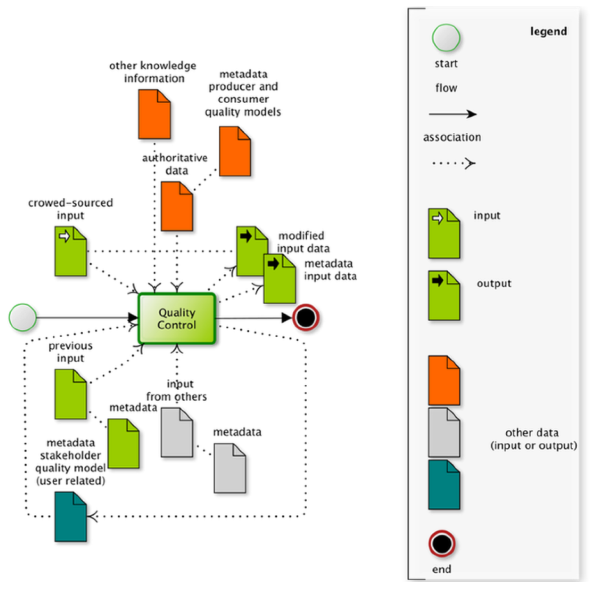
2. Quality Assurance and Quality Control Framework

The COBWEB project aimed at designing and building a generic interoperable e-infrastructure facilitating the collection and curation of CS data for future usage in environmental monitoring [12]. As part of this e-infrastructure, QA plays an important role, either during or after data capture. A QA procedure is designed using the QA workflow Authoring Tool (QAwAT), a web interface of the QA framework. It is based upon a workflow editor that uses the Business Process Modelling Notation (BPMN) standard, a standard for graphical notation for specifying business processes (similar to a flow chart) www.bpmn.org. QAwAT enables the selection of QC tests by the stakeholder, which are then combined and chained to form a QA procedure for their CS survey [37,38]. To ensure interoperability, the QCs are implemented as Web Processing Service (WPS) processes. The OGC Web Processing Service standard provides rules for standardizing how inputs and outputs for invoking geospatial processing services are defined. Each QC takes the CS data and their metadata (including any existing quality valuations) as input, and performs processing and geoprocessing on these data, producing or updating the quality metadata of each single observation of the CS data (Figure 1). This process may involve other data sources, e.g., authoritative data, EO data, social media.
As part of the COBWEB platform, the QAwAT offers flexibility in designing, recording and executing a quality assurance workflow; it enables communication and dialog between stakeholders and provides metadata on metaquality in a machine-readable format (a BPMN file).
Figure 1 shows a QC conceptualized in a BPMN diagram, as a QA workflow with a single task. This representation of a single QC and a full workflow, are based upon the same principle, which might use additional BPMN artifacts, such as conditional flow, parallel gateways or inclusive gateways. Using the BPMN standard, the full workflow for QA can be displayed with or without inputs (as in Figure 2, and Appendix A Figure A1). This displays all the involved artifacts, and the quality elements created and updated during the execution of the workflow, which are shown as annotations: Vol as volunteer referring to the stakeholder quality model, Obs referring to the Producer quality model, and Auth to the consumer model. These annotations, only used when communicating graphically between stakeholders, are conformant to the BPMN standard.
The metadata on data quality belongs to three different quality models (see Appendix B for a full description): the producer model, generating the spatial data quality from the ISO19157, the consumer model following the principle of the user feedback model (Geospatial User Feedback Standard Working Group www.opengeospatial.org/projects/groups/gufswg) and the stakeholder quality model [26,36]. The ISO 19157 establishes the principles for describing the quality of geographic data Qualifying each citizen volunteer, the stakeholder quality model produces quality elements that are updated at each new participation in a survey (from running the associated QA) but current values are kept associated with the observation when it is made by this citizen volunteer. Not only can the current values of the stakeholder quality model influence, as weighting factors, the quality assessment for the other quality models, for a new data captured by this citizen (seen as an observation made by the sensor “this citizen”), but they will also evolve from the processing and rules within each QC. All three quality models use an encoding that follows the ISO19157 schema, with a scope to link “citizen” to the current observation.
The QA framework proposes 7 categories of QCs as 7 Pillars for quality assessments of CS data (Table 1). This categorization into 7 pillars helps in the development of geoprocesses and in the composition of the workflow. They represent the top of an ontology for the QCs for CS quality assessments. The 7 Pillars further extend the classification of quality assessments proposed in previous work by Goodchild & Li [22]: “the crowdsourcing approach” (validation in reference to the rest of the crowd); “the social approach” (validation using expert peers or trusted peers); and “the geographical approach” (validation involving the geographical context). Several QCs accessible have been developed, and are available within the WPS repository (implemented either in Java or as R scripts). A screenshot and video of the interface can be viewed in the GitHub repository (https://github.com/cobweb-eu/workflow-at) and shows composition of a QA workflow, including choosing a QC from a list of QCs (classified as one of the 7 pillars), populating the necessary input parameters and input data, then continuing to instantiate the workflow.
The following section illustrates the usage of this QA framework for CS data from the JKW survey in the SNP.

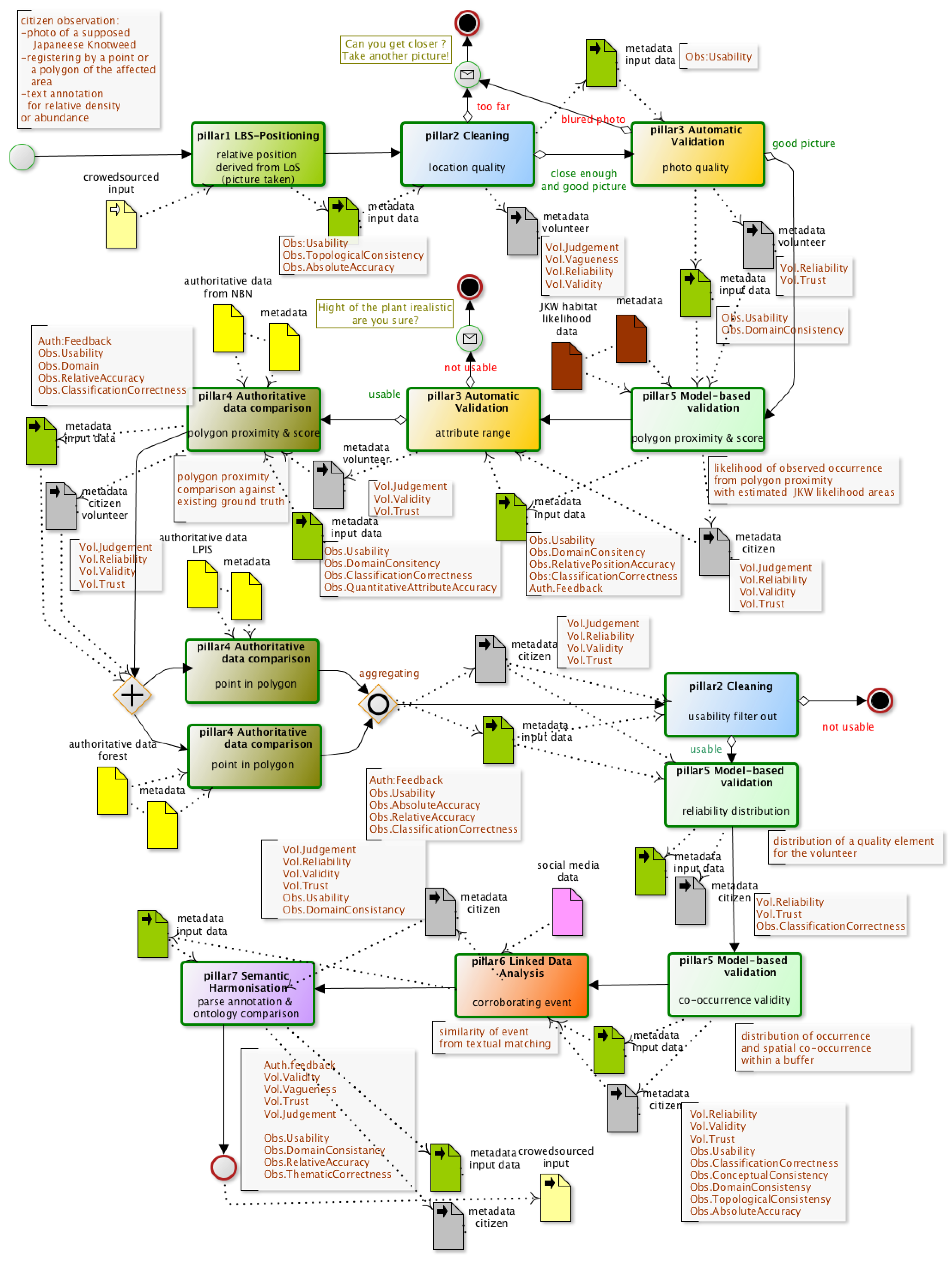
3. Designing the Japanese Knotweed Quality Assurance

The COBWEB app [12] was used to record the CS data, with a single observation containing positional information, photos of the reported JKW, along with bearing and tilt angle parameters given by their smartphone, and the citizen’s estimates of the heights of the plants. The citizens were also asked to report their distance to the declared JKW occurrence (see Appendix C), and an approximation of the area covered by the JKW.
The diagrammatic QA workflow for the JKW study (Figure 2) was designed following initial discussions with the stakeholders. Further engagement led to some modifications to the rules within a QC, for instance “JKW does not grow in the forest or in managed land”, leading to QCs in Pillar 4 (Authoritative data comparison) using forest and managed land data (termed LPIS in the diagram). The Pillar 4 Point in polygon QC (pillar4.PointInPolygon) tests the inclusion of a point, taking into account positional accuracy of both the point and the authoritative data, and concludes first on the usability, topological consistency and domain consistency. Then, depending on the type of attribute attached (if mentioned), i.e., classification or quantitative or non-quantitative, and of the agreement looked for (“must be in” or “must be not in”), updates the corresponding ISO19157 elements, e.g., thematic classification correctness.
Although the ordering of the pillars in Table 1 is not compulsory when composing any QA workflow, there is often a natural succession of QCs. This subjective order follows from “topological and location concerns for the observation”, with typical QCs in Pillar 1 (positioning) and Pillar 2 (Cleaning), to “content concerns”, with Pillar 3 (Automatic Validation) for photo quality evaluation. Next follows Pillar 5, with the modeled data from EO (Model-based validation), attribute range (from Pillar 3), and the authoritative data of known verified occurrences (Pillar 4, Authoritative data Comparison) with the authoritative data sourced from the National Biological Network (NBN), and then excluding rules in Pillar 4 for forest and managed land. Following this, “content concerns” comes from the consistency of the answer by comparing this citizen to the other citizen scientists (Pillar 5 for reliability distribution and co-occurrence validity). Then enlarging the comparison to other data sources from the crowd with a QC in Pillar 6 (Linked Data Analysis), and finally a normative assessment for the photo annotation from a QC in Pillar 7 (Semantic Harmonization).
The EO data used in Pillar 5 Proximity Suitability Score QC (ProximitySuitabilityScore) are considered as semantically equivalent to the CS data. Observing JKW a citizen also identifies a high-risk zone (without delineation). The risk is taken as the classification correctness reached by the citizen, 1 if CS is considered to be ground truth, but could be lower depending on the quality and trust of these CS data. The fact that, if more citizens make the same observation it would increase the local quality of the EO data itself, is not the purpose here. Nonetheless, these co-occurrences made from the CS viewpoint are used in the QA (qualifying the CS data), as increasing the quality of the observation and credibility of the citizen. Where the EO product estimates an area with a high-risk value, one could expect (with a high probability) that a nearby citizen scientist would report a JKW occurrence. Nonetheless, the survey was not set up to allow regular reporting of occurrences or absences of JKW, i.e., the citizen would be prompted to report at regular time intervals or set distances as well as allowing spontaneous reporting. Therefore, the equivalence of CS and EO information is directly valid only for areas of declared occurrences from citizens (true and false positive statistics). False negatives were obtained indirectly, using the verification process; however, the sample was considered unbalanced, with only 10% incorrect observations. This paper does not include a comment on the method of EO data product generation that predicted the risk of occurrence of the JKW, as this is not its focus; only what the EO product represents is required, either when using it in the QA workflow as in Figure 2 (see Section 5) or when using CS to validate it (see Section 4).
Taking the values of the EO data as suitability scores, which are measures of likelihood of occurrence, the pillar 5 Proximity Suitability Score QC (ProximitySuitabilityScore), highlighted in Figure 2, computes a weighted summary (mean or max) of the values found within the nearby polygons of the EO data product, to the current CS observation. It then assigns these to the classification correctness quality element of that current CS record. Usability and positional accuracy (from accuracies of the polygons) are updated during the process, depending on the score obtained during the comparison to a chosen quality element with simple threshold rules.
For the remainder of the paper, there is a distinction made between the entire QA (as shown in Appendix A Figure A1), and the QA without the Pillar 5 (Model-based Validation) QC, which uses the EO data (for the risk of JKW). The latter is highlighted in Figure 2. Note, for both situations, the QCs in Pillar 6 (Linked Data Analysis) and Pillar 7 (Semantic Harmonization) were not used due to insufficient, relevant additional data but were left in Figure 2 as part of the established QA workflow for JKW. Running the QA workflow produced quality values for each recorded observation in the CS data. Summaries at dataset level can be made but in the remainder of this paper, CS data quality is considered at individual record level (each citizen’s observations). For example, the Data Quality element Classification Correctness (DQ_ClassificationCorrectness), for the CS data from this study, is a vector of 177 values, each ranging between 0 and 1.

4. Using Citizen Science for Earth Observation Validation

Within the approach for validating an EO data product from other data sources, CS data can play an important role for the validation itself. This can be within a partial opportunistic scheme or providing a training sample as a ground truth, e.g., for a supervised classification algorithm. Although all the data quality elements are potentially important for the future usage of the CS data, the main quality of interest here is the classification correctness (from ISO19157). Each of the 177 CS data records were verified by an expert, who from photo examination, declared 16 as incorrectly identifying a JKW presence. Further information on the JKW co-design study can be found on the COBWEB website (https://cobwebproject.eu).

4.1. Without Quality Assurance of the Citizen Science Data

Without a means of QA, there is total uncertainty concerning the quality of the CS data, so either the end user would have to blindly trust the data by artificially assigning a classification correctness of 1 (as degree of agreement) for each observation, or they would have to assign 0.5 as degree of agreement (neither correct nor incorrect). A value equal to or below 0.5 is not usable for validation, so to use the CS data without QA implies a full degree of trust.
As each CS observation should be associated in the EO data as a high-risk point of observing JKW, the “score” obtained in the Pillar 5 QC (Proximity Suitability Score (ProximitySuitabilityScore)) alone is a validation measure for the EO, of high risk zones. When this score is high, the single CS observation is not too far from a polygon of the EO data attributed as high risk of JKW presence. Therefore, this CS observation implicitly declares the EO data as accurate in this zone. However, if this CS observation has been verified as incorrectly declaring the presence of JKW the EO polygon contributing to a high-risk score can also be considered as incorrect: a commission error (i.e., excess data present in a dataset, measured here as number of excess items in the dataset or sample in relation to the number of items that should have been present (ISO19157); this is also the false positive rate). When the score obtained for a verified as correct single CS data is low, this infers that the EO data has an omission of high-risk polygons in this zone (i.e., data absent from the dataset, measured here by the number of missing items in the dataset or sample in relation to the number of items that should have been present (ISO19157); this is also the false negative rate). Applying these rules for the whole CS data sample, the findings are:
  • CS data with no score (25/177) and score <0.2 (20/177) represent an omission for high-risk zones of 45/177 (25%) and correcting for ground truth gives 39/161 (24%).
  • CS data with score >0.5 represent accurate areas, 120/177 (68%), but 10/120 (8%) points wrongly identified JKW so a corrected accuracy of 110/177 (62%) with a commission of 8%.
The accuracy measures above (68% and 62%) represent the validation of high or medium risk zones only but these accuracy measures are relative to this very opportunistic sample that the CS data represents. Note, the maximum accuracy one can obtain using this sample of 177 is 91%, due to 16/177 being incorrectly identified JKW observations.
The commission accuracy for the “low” or “no” risk zones identified by the EO data can be calculated with the same algorithm by inverting the risk values, giving 3/177 (2%) or 3/161 (2%) corrected. Obviously, here the sample size of 177 control data points can be considered too small in comparison to the number of segmented zones within the EO data. (Note the 16 incorrect observations would also contribute to defining the accuracy of the “no risk” zones but with a very small sample). However, the nature of CS data is such that optimal sample numbers and spatial distribution are rarely obtained, e.g., areas inaccessible by the citizens.
If this CS sample cannot be used to assess the validation of the EO data, one can nonetheless expect that if the EO data were accurate, with 10% omission for the high-risk zones, this omission value should be observed for any sample coming to challenge this validation. The CS sample (taken as fully accurate) gave an omission of 25% (24% corrected).

4.2. With Quality Assurance of the Citizen Science Data

As expressed above, CS data identifying invasive species without quality is taken either as truth in full trust (classification correctness implicitly set to 1) or full uncertainty (classification correctness set to 0.5). Therefore, when starting any QA, the quality elements measured from a level of agreement, start with a value of 0.5. Due to the small number of incorrect JKW in the verification (16/177), a QA matching the verification performance should not change the above accuracy statistics for the EO data. However, it is established that expert validation itself is not always fully accurate. As the QA is based upon external assessments, and a set of rules, it will also be discriminating the correct observations, and changes will occur in these statistics when based upon selecting only high quality CS data. Note that here the QA may discard (give a low-quality value) for an accurate JKW observation, e.g., the observation is located too close to forest, therefore being “unreliable” as defined in the QA rules.
The QA from Figure 2, was then executed without the inclusion of the Pillar 5 QC test, which used the EO data product. Selecting only CS data with usability or classification correctness above the chosen threshold of 0.7, the findings in 4.1 become:
  • CS data with no score (10/66) or score <0.2 (9/66) represent omission areas of 19/66 (29%).
  • CS data with score >0.5 represent accurate areas, 41/66 (62%).
Comparing these results with those based upon ground truth, reveals a similar global accuracy (for the high and medium risk zones), 62%, but a more pessimistic omission rate 29% vs. 24%. The sample size after selection, of at least 0.7 in usability or classification correctness, can be put into question. Nonetheless, it shows that qualified CS data could be a substitute to verified CS data.

4.3. With Line of Sight Correction in the QA for the Citizen Science Data

One important consideration when deriving the data quality is that the geoprocessing algorithms are based upon the location of the citizen (of their smartphone), and not the actual position of the observation, which is the aimed point on the ground when taking the photo (line of sight (LoS)). In the QA described in Figure 2, the first QC, Pillar 1 Relative Position Line Of Sight QC (RelativePositionLineOfSight), uses the LoS but aims to investigate the quality of the topological consistency. The process uses a Digital Elevation Model (DEM), and the device’s bearing, tilt and position information to compute the LoS [39]. For this case study, the Natural Resources Wales LiDAR 2 m resolution Digital Surface Model was used for the DEM input. The QC assesses whether the distance of the citizen to the declared observation is too far or not (see the pseudo code given in Figure 3), and has the option of correcting the position of the observation by replacing it with the line of sight base point, under certain conditions. With this option chosen, the quality values may differ considerably (see Section 5) during the rest of the QA.
The pseudo-code in Figure 3, as does the other QCs given in Appendix A Table A1, gives some insight into how The 7 Pillars of QC have been designed and coded. According to the Pillar concept, QC test undertakes some computation based on its input data (for Figure 3 this is the LoS point and its distance to the volunteer), which is then passed onto bespoke rules estimating relevant quality element values.
Using a threshold distance of 5 m to define the topological consistency (e.g., a swap from 8.3 m using p-below set to 0.6, if the accuracy is similar to the initial average position accuracy of 13 m), the findings above, still selecting only CS data with usability above 0.7, become:
  • CS data with no score represents omission areas, 0/72 (0%).
  • CS data with score >0.5 represent accurate areas, 72/72 (100%), correcting for ground truth gives 67/72 (93%).
  • CS data with score <0.2 (which was the low risk value in the EO data) represents an omission rate of 0/72 (0%).
The LoS correction affected 38 out of 177 CS data records, i.e., where the LoS gave a result. No estimation is returned when either the line of sight does not reach the DEM within a 1000 m distance, or the tilt angle is inadequate, or when the DEM has an issue (no data value encountered, due to holes, etc.) [39]. Out of the 38 points, 26 obtained a topological consistency below 0.6, i.e., the citizen was identified as being too far from the observation. Forcing a replacement, for example by setting p-below to 0.99, could introduce some error propagation effects, as the uncertainties of the tilt and bearing can be potentially important (see Table 3 in the Discussion section). Overall, comparing results in Section 4.2 and Section 4.3, the LoS base point correction improved the EO accuracies.

5. Using Earth Observation to Improve Citizen Science Data Quality

In Section 4.2, the QA from Figure 2 was used without the inclusion of the Pillar 1 Proximity Suitability Score QC (ProximitySuitabilityScore) as highlighted in Figure 2, which uses the EO data product. Comparing the quality element obtained with and without running this particular QC gives some indications of the usefulness of such an EO data product, and whether or not this can be used directly in environmental policy making, even if the EO product itself is not considered as “perfect”. The plots in Figure 4 are density plots of the quality element values derived after running the QA (entirely or without that QC), and were obtained from the R function density(): the y-axis is the density value as defined by this function. Raw observations have also been overlaid for each group, displaying the observed distributions of values (no y-axis for these).

5.1. CS Data Validation

The first row of plots in Figure 4 corresponds to the values used in Section 4.2, i.e., without the QC in Pillar 5 involving the EO data. Being able to test the performance of the QA with verified CS data, also completes the EO to CS data validation.
Figure 4 shows that, without the Pillar 5 QC involving the EO data product, the data resulted in too many correct JKW observations with low quality values. The densities are also very similar between the two groups, even though the densities of very low quality values are higher for incorrectly identified JKW observations. However, one must be cautious, as the sample size difference between the two groups introduces a bias when looking at the densities. Running the entire QA corrected these two aspects to some degree, as the densities of correctly identified JKW observations have a mode towards high qualities (plots labeled “Entire QA”).
The distributions also appear more in agreement with correct and incorrect JKW observations, as uncertainties (0.5) remain higher for incorrect JKW observations, and the density of high qualities is higher for correct JKW observations. Nonetheless, low quality values are still given to a considerable number of correct JKW observations. This could be an indication for adding more tests into the QA workflow, or adjusting some parameters used in these QCs. Beside a calibration issue, there may also be a sensitivity issue due, for example, to position uncertainty or the quality of the authoritative data used in the different QCs. Note that a simple t-test for classification correctness resulted in a mean comparison of 0.65 for correctly identified JKW, and of 0.57 for incorrectly identified JKW (p value = 0.09). For the QA without LoS correction, the same t-test gives: correct JKW, 0.65 incorrect JKW 0.58 (p-value = 0.10). This solely demonstrates the usefulness of the QA in discriminating data quality. Moreover, the same t-test for the quality results obtained without the QC in Pillar 5 (Model-based Validation), involving the EO data, is not significant (p value = 0.3), therefore highlighting the importance of this Pillar 5 QC and supporting EO data product, in the QA process.

5.2. Iterative Paradigm

As seen in Section 5.1, despite the indication that the EO data quality is not high (Section 4), the CS data quality will only improve when used in the QA. Provided the EO data does not have high commission (false positive rate) and omission (false negative rate) errors, this would generally work, otherwise to some extent, the errors will propagate into the CS qualification. Here, this could be the cause of high quality values for some incorrect JKW observations (false positives), as well as low quality for some correct JKW observations. Note that the differences in commission for high and low risk categories could be challenging, therefore, only using the extreme risk categories within EO data for a JKW risk product, would be a better choice for QA.
The EO algorithm could also utilize the qualified CS data as additional evidence to support the algorithm (as a training sample). From the iterative process that could result, the EO data zones where the CS data have been validated would then conflate appropriately to the CS data, ensuring better agreement of CS with EO data. Providing the QA makes use of the additional “qualifying rules” related to EO data product, this iterative process would be alternating (i) the EO supervised algorithm using the CS of high quality, and (ii) the QA for the CS data including the EO data product for JKW risk obtained in (iii), where a threshold of high quality is fixed after the first iteration. Once validated, the new CS data collection, used as supplementary training samples, could also generate some benchmarking requirements when new EO imagery data would be needed, i.e., using the goodness of fit of the EO algorithm. Within an environmental monitoring scheme, EO and CS would then be complementary.

6. Discussion

With the aim of providing relevant metadata for CS data along with the provenance of the metadata on data quality, i.e., the metaquality encapsulated in the QA workflow, the results shown in the preceding sections are promising. They show also the benefit of using qualified CS data to validate the EO data. However, there are some important and notable limitations. The EO data validation must be seen more as a confirmation rather than an assessment of the validation because the CS data are an opportunistic sample not controlled for EO validation. Nonetheless, for the user’s accuracy, and whether the sampling is controlled or not, as long as no evidence of introducing a bias in omission or commission can be established, the values obtained reflect a level of quality present in the EO data product. If the sample size of the verified data (ground truth) were large enough and balanced in potential presence or absence of the INNS, assessing the omissions and commissions of the EO data (as in Section 4), using qualified CS data instead of only the verified data has nonetheless, proven to be useful. Moreover, correcting the position of the occurrences using the LoS improved the results in EO confirmatory validation (Section 4.3, even though the DEM accuracy as well as tilt and bearing accuracy may induce a propagation of errors. The distance to the observation as declared by the volunteers can have variable quality and its comparison to the LoS distance showed large differences (see Appendix C Table A5).
If, overall, the QA results discriminated the correct and incorrect JKW occurrences well (true positive versus false positive), the current QA performance did not seem able to adequately identify a single observation as correct, or not, from its resulting qualities. The number of QCs used, their characteristics, their order in the QA workflow, the positional accuracy sensitivity for both the observed data and the external data used, along with the parameters chosen in the QC (such as threshold distances) are contributing to the QA outcome, with potential issues due to calibration and error propagated through the defined QA workflow. One could expect that increasing the number of QCs would diminish its sensitivity. Cancelling out the assessment for a given QC, if the quality metadata linked to the external data do note reach a certain level, would diminish error propagation while highlighting inadequacy. Down weighting the impact of new quality values when updating can also be a less drastic solution to low quality external data used in the QA. Note, the concern was only on qualifying the declaration of occurrence of the JKW plant; however, combining evidence across other available information can lead to better qualifying. For instance, the extent of the JKW at a declared occurrence and its potential agreement with the EO data product may be useful, i.e., it can be reasonably thought that the confidence in the risk given by the EO data product is increased as the extent detected by the EO algorithm becomes larger. This also raises concerns about the use of EO to bring evidence of the JKW or another INNS without appropriate spatial and temporal resolution for the detection of early spread [40]. A citizen scientist may detect a very early spread of JKW, observing a very small extent that EO would be unable to achieve. These considerations have impacts on both, EO for CS or CS for EO validation paths.
A further limitation is the number of volunteers used (34) and the number of observations (177), and reflected the relatively small-scale co-design type project. One way of increasing the number of observations would have been to regularly ask the citizen scientist to identify, at their current location, the occurrence or absence data for JKW. This would also have resulted in a better estimation of commission in the EO data, along with a better calibration of the citizen’s qualities as a sensor, i.e., trust, reliability.

7. Conclusions

As an alternative to a costly and not necessarily reliable “verification process” often used in biodiversity Citizen Science (CS) surveys, this paper investigated the role and usefulness of an automated Quality Assurance workflow process based on 7 Pillars of Quality Controls, and the three quality models introduced by the COBWEB project [12]. Besides the flexibility this approach offers for curation of CS data, a case study and results investigating citizen reporting of an invasive species (Japanese knotweed) are reported. Specifically, using informative earth observation data within the quality assurance workflow, in relation to the occurrences of Japanese knotweed, even when of low quality, improves the CS quality assessment, i.e., it enables better discrimination between correct and incorrect JKW occurrences. Conversely, using qualified CS instead of raw CS data resulted in increased user’s accuracy for the earth observation data. In Groom et al. [41], the authors advocate an open data approach concerning the invasive non-native species (INNS), in order to facilitate policy and management. As the CS data are unlikely to be of high quality, and verification from experts is not always viable (or not possible for all CS data), the automatic quality assurance presented in this paper could be beneficial. Several limitations have been highlighted, however, and indications for potential remedies to the sensitivity of the quality assurance process were given. Multiple criteria selection on the quality elements, to validate CS data, could compensate for the weaknesses of the QA workflow used. Trustworthiness is used in many CS data collection systems, such as iSpot [42] and CoralWatch [27] as proxies for verification or in combination with other QA approaches to highlight potential re-use. Addressing several dimensions related to trustworthiness, the stakeholder quality model plays a role in qualifying the volunteer’s observations. A QC can use those quality values as weights for updating the other quality elements. It is expected that the flexibility provided by this QA framework, along with its principles, would guide the development of new QCs within the given pillars system as in the composition of workflows from stakeholders. In order to achieve robustness of the qualifying process, performing a pilot study in order to test the composed workflow QA on a verified sample is recommended as a necessary step before being used for a complete CS study.
The QA framework presented is applicable in other environmental monitoring contexts for which EO data and CS data can be complementary. A typical example can be land use mapping with an emphasis on crop identification for agricultural land. Being able to appropriately combine multiple source of information with EO data, including CS data is becoming a high priority in initiatives such as the Copernicus program directed by European Commission [43]. Citizen observatories, where citizen science data are empowering directly the citizens, for example in reaction to the EO available, play an important role in this “Copernicus chain” (from EO data to usable information) [43]. It is acknowledged that a successful implementation of this “Copernicus chain” would require attention to data quality. The QA framework presented in this paper could contribute to this success.

Acknowledgments

This research has received funding from the European Union Seventh Framework Programme (FP7/2007–2013) under grant agreement number 308513.

Author Contributions

C.C., Cr.H. and Ch.H. co-designed the JKW experiment. D.G.L., J.F.R. and M.J.J. designed the QA framework. D.G.L. and J.W. designed the JKW. QA. J.W. provided the EO data related to JKW risk. D.G.L. and J.F.R. implemented the QA. D.G.L. structured the paper, performed the analysis and wrote the paper. D.G.L, Cr.H., J.W. and J.F.R finalized the paper.

Conflicts of Interest

The authors declare no conflict of interest.

Abbreviations

The following abbreviations are used in this manuscript:
CIRColored Infra-Red
COBWEBCitizen OBservatory WEB
CSCitizen Science
DEMDigital Elevation Model
EOEarth Observation
FP7Framework Program 7
IASInvasive Alien Species
JKWJapanese KnotWeed
INNSInvasive Non-Native Species
LiDARLight Detection And Ranging
LoSLine of Sight
QAQuality Assurance
QAwATQuality Assurance workflow Authoring Tool
QCQuality Controls
SNPSnowdonia National Park
VGIVolunteered Geographic Information

Appendix A

Figure A1. Entire QA workflow of Figure 2: annotated BPMN where each QC is labeled with its pillar number, pillar name, and a short textual illustrating the semantic of the process. The annotations in brown list the quality metadata output at each step. (see www.bpmn.org for BPMN artifact descriptions).
Data 02 00035 g005
Table A1. Pseudo-code of the QCs used in Figure 2 with a short description including input and output.
Pseudo CodeShort DescriptionQuality elements metadata created or updated:
DQ ISO19157 producer model
GVQ GeoViQUA’s feedback model (simplified)
CSQ COBWEB’s stakeholder model
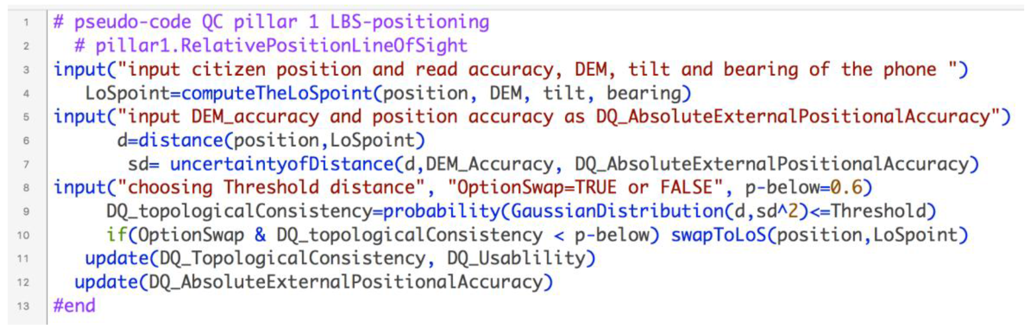
pillar1.LocationBasedServicePosition.RelativePositionLineOfSight
#start
input("citizen position, DEM, tilt and bearing of the phone ")
LoSpt=computeTheLoSpoint(position, DEM, tilt, bearing)
input("input DEM uncertainty and position uncertainty")
  d=distance(position,LoSpoint)
   sd= uncertaintyofDistance(d,DEM_Accuracy, DQ_AbsoluteExternalPositionalAccuracy)
input("choosing Threshold distance", "OptionSwap=TRUE or FALSE", p-below=0.6)

DQ_topologicalConsistency=probability(GaussianDistribution(d,sd^2)<=Threshold)
  if(OptionSwap & DQ_topologicalConsistency < p-below) swapToLoS(position,LoSpoint)
 update(DQ_TopologicalConsistency, DQ_Usablility)
  update(DQ_AbsoluteExternalPositionalAccuracy)
#end
Compute the line of sight, aiming point and distance to it. Swap to LoS point under certain conditions

DEM
ThresholdDistance
p-below
OptionSwap
DQ_UsabilityElement
DQ_TopologicalConsistency

-LoS.point                     / DQ_AbsoluteExternalPositionalAccuracy
with scope defined as “LoS” .
pillar2.Cleaning.LocationQuality
#start
input("input citizen position, DQlevelThreshold, PosUnThreshold, methods")
 for each observation {
  for each method in methods {
   DQ_usability=evaluateRule(DQ_AbsoluteExternalPositionalAccuracy,
DQ_usability, DQ_topologicalconsistency, DQ_conceptualconsistency)
  } }
 update(CSQs)
#end
According to the study requirement check if position is correct and/or can be corrected
methods:
“pillar1.WithinPoly”, ”pillar1.LineOFSight”, “pillar1,ContainsPoly”, “pillar1.GetSpatialAccuracy”,”
pillar4.or pillar1.DistanceTo”
DQlevelThreshold
PosUncertaintyThreshold
DQ_UsabilityElement
CSQ_Vagueness
CSQ_Judgement
CSQ_Reliability
CSQ_Validity
pillar3.AutomaticValidation.PhotoQuality
#start
input("input citizen captured photo, blurThreshold," )
   edgeImage=LaplaceTrasnform(photo)
    usable=evaluateRule(edgeImage, blurThreshold)
update(DQ_usability, DQ_DomainConsistency, CSQ_judgement, CSQ_trust)
message(usable)
#end
Test on sharpness of the image using the method of edge detection from Laplace transform.

BlurThreshold
DQ_UsabilityElement
DQ_DomainConsistency
CSQ_Reliability
CSQ_Trust
-dynamic:
<message> “Can you take another picture?”

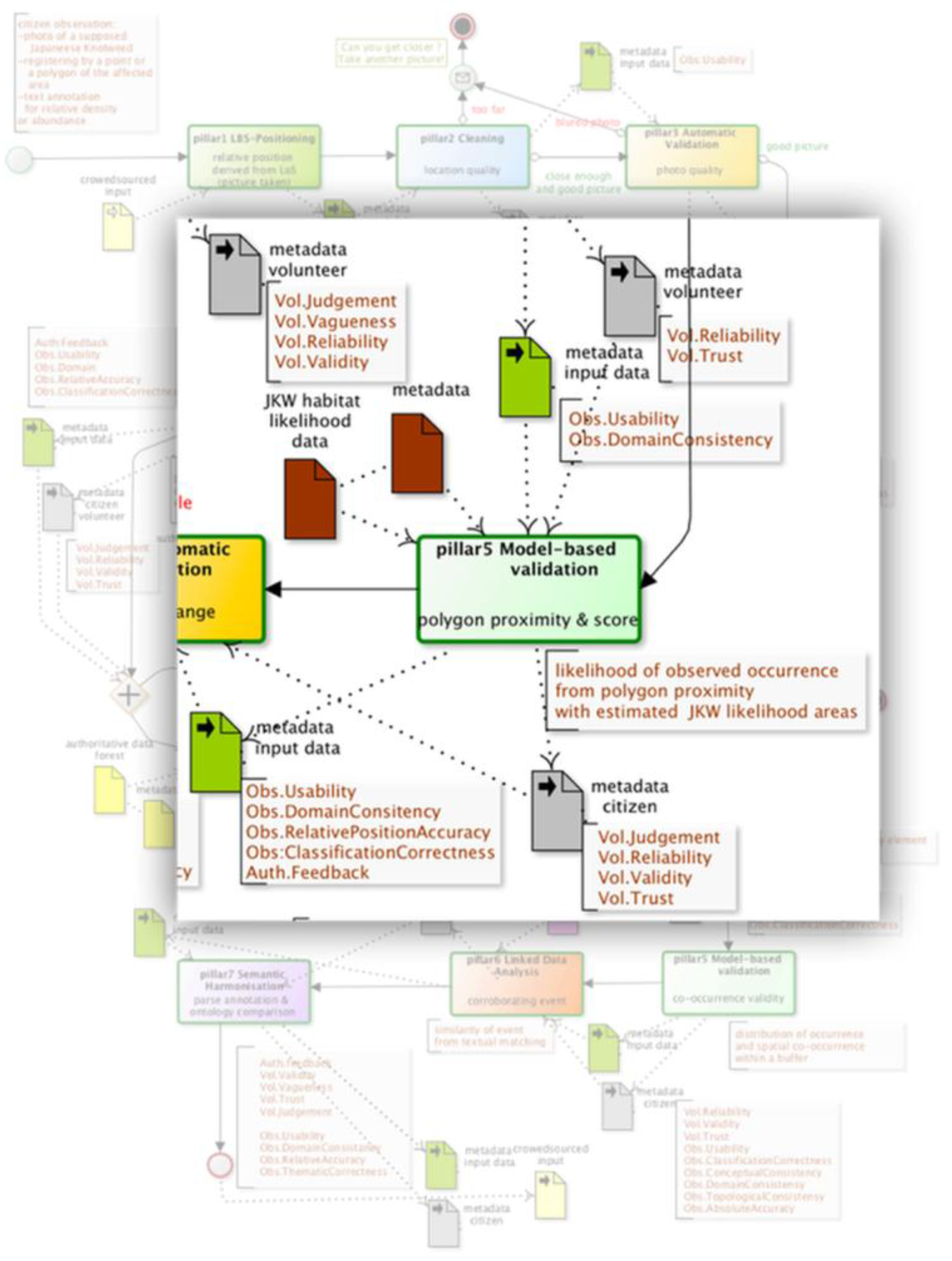
pillar5.Model-basedValidation.ProximitySuitabilityScore
#start
input("input citizen position, buffersize, attribute")
  ProximPol=findNearby(buffersize)
   score=summaryMeasure(calculweightDistance(ProximPol),values(ProximPol, attribute))
updateRules(DQs,CSQs,GVQs, score)
#end
Deriving the likelihood of the observed occurrence (citizen captured data) from polygon proximity to a model-estimate one (e.g. suitability likelihood)

modelled data
attribute
buffersize

DQ_UsabilityElement
DQ_ThematicClassificationCorrectness
DQ_AbsoluteExternalPositionalAccuracy
DQ_RelativeInternalPositionalAccuracy
GVQ_PositiveFeedback
GVQ_NegativeFeedback
CSQ_Judgement
CSQ_Reliability
CSQ_Validity
CSQ_Trust
pillar4.AuthoritativeDataComparison.ProximitySuitabilityScore
#start
input("input citizen position, buffersize, attribute")
  ProximPol=findNearby(buffersize)
   score=summaryMeasure(calculweightDistance(ProximPol)
updateRules(DQs,CSQs,GVQs, score)
#end
Deriving the likelihood of the observed occurrence (citizen captured data) from polygon proximity to a given authoritative data (e.g. existing observed occurrences)
Authoritative data
Buffersize
Note: comparing to pillar5 attribute value is 1 as authoritative data.

DQ_UsabilityElement
DQ_DomainConsistency
DQ_ThematicClassificationCorrectness
DQ_NonQuantitativeAttributeCorrectness
DQ_AbsoluteExternalPositionalAccuracy
DQ_RelativeInternalPositionalAccuracy
GVQ_PositiveFeedback
GVQ_NegativeFeedback
CSQ_Judgement
CSQ_Reliability
CSQ_Validity
CSQ_Trust
pillar4.AuthoritativeDataComparison.PointInPolygon
#start
input("citizen observation, thematicAgreement, AuthData, Buffersize")
InPol=evaluateIn(observation.DQ_AbsolutePositionInternalPositionalAccuracy, AuthData.DQ_AbsolutePositionInternalPositionalAccuracy, AuthData, Buffersize)
  IniScore=EvaluateOverlapAreas(InPol, observation, uncertainties)
updateRules(DQs,CSQs,GVQs, IniScore)
   if(not InPol) {
  ProxPol=evaluateNear(Obs.DQ_AbsolutePositionInternalPositionalAccuracy, Auth.DQ_AbsolutePositionInternalPositionalAccuracy)
  ProxScore=Evaluate(ProxPol, Obs, uncertainties)
    updateRules(DQs,CSQs,GVQs, ProxScore)
    }
#end
given the position and its uncertainty checking if a point belongs to a polygon then concluding on relative position accuracy and 'relative' semantic therefore usability and attribute accuracies

Authoritative data
ThematicAgreement
DQ_UsabilityElement
DQ_ThematicClassificationCorrectness
DQ_NonQuantitativeAttributeCorrectness
DQ_QuantitativeAttributeAccuracy
DQ_AbsoluteExternalPositionalAccuracy
DQ_GriddedDataPositionalAccuracy
DQ_RelativeInternalPositionalAccuracy
GVQ_PositiveFeedback
GVQ_NegativeFeedback
CSQ_Judgement
CSQ_Reliability
CSQ_Validity
CSQ_Trust

Appendix B

The three quality models used in QAwAT are given Table A2, Table A3 and Table A4.
Table A2. Producer Quality Model (ISO19157); all the elements of the standard can potentially be used, even though they were initially designed for authoritative data.
DQQuality Element DQ_Definition Extracted from the ISO19157
01UsabilityElementDegree of adherence to as specific set of data quality requirements.
02CompletenessCommissionExcess data present in a dataset.
03CompletenessOmissionAbsence of data in a dataset.
04ThematicClassificationCorrectnessComparison of the classes assigned to features or their attributes to a universe of discourse (e.g., ground truth or reference data).
05NonQuantitativeAttributeCorrectnessWhether a non-quantitative attribute is correct or incorrect.
06QuantitativeAttributeAccuracyCloseness of the value of a quantitative attribute to a value accepted as or known to be true.
07ConceptualConsistencyAdherence to rules of the conceptual schema.
08DomainConsistencyAdherence of values to the value domains.
09FormatConsistencyDegree to which data is stored in accordance with the physical structure of the dataset.
10TopologicalConsistencyCorrectness of the explicitly encoded topological characteristics of a database.
11AccuracyOfATimeMeasurementCloseness of reported time measurements to values accepted as or known to be true.
12TemporalConsistencyCorrectness of the order of events.
13TemporalValidityValidity of data with respect to time.
14AbsoluteExternalPositionalAccuracyCloseness of reported coordinate values to values accepted as or being true.
15GriddedDataPositionalAccuracyCloseness of gridded data spatial position values to values accepted as or being true.
16RelativeInternalPositionalAccuracyCloseness of the relative positions of features in a dataset to their respective relative positions accepted as or being true.
Table A3. Simplified Consumer Quality Model (GeoViQUA www.geoviqua.org): for COBWEB the simple concept of positive and negative feedback is kept but as automatically generated by the QCs.
GVQ_Quality Element GVQ_Definition
01PositiveFeedbackNumber of positive feedbacks to the used data
02NegativeFeedbackNumber of negative feedbacks to the used data
Table A4. Stakeholder Quality Model (COBWEB): qualifies the citizen volunteer in order to influence further confidence in a particular citizen’s observations when deriving the producer quality model values.
CSQ_Quality Element CSQ_Definition
01VaguenessInability to make a clear-cut choice (i.e., lack of classifying capability).
02AmbiguityIncompatibility of the choices or descriptions made (i.e., lack of understanding, of clarity).
03JudgmentAccuracy of choice or decision in a relation to something known to be true (i.e., perception capability and interpretation).
04ReliabilityConsistency in choices / decisions (i.e., testing against itself).
05ValidityCoherence with other people’s choices (i.e., against other knowledge).
06TrustConfidence accumulated over other criterion concerning data captured previously (linked to reliability, validity and reputability).
07NbControlsTotal number of controls over all contributions of this volunteer.

Appendix C

Table A5. Comparison of the citizen’s declared versus estimated from LoS distances (for 38 pts) of the citizen to declared invasive species.
Declared DistanceN (Total 177)LoS Distance (38/177)
Close (<1 m)73N = 10 out of * 73,
Min. 1st Qu. Median Mean 3rd Qu. Max.
1.5 3.1 6.5 12.7 15.0 59.3
Nearby (1 m–3 m)30N = 9 out of * 30,
Min. 1st Qu. Median Mean 3rd Qu. Max.
3.5 5.8 14.8 213.5 516.9 687.8
Far (3 m–10 m)39N = 13 out of * 39,
Min. 1st Qu. Median Mean 3rd Qu. Max.
1.5 2.0 16.5 125.0 175.7 642.3
Very far (>10 m)34N = 6 out of * 34,
Min. 1st Qu. Median Mean 3rd Qu. Max.
1.5 2.4 5.0 11.3 6.9 47.1
missing1-
* not all estimations gave a result (see Section 4.3).

References

  1. DEFRA. UK Biodiversity Indicators in Your Pocket. 2015. Available online: http://jncc.defra.gov.uk/page-4229#download (accessed on 30 July 2016).
  2. Williams, F.; Eschen, R.; Harris, A.; Djeddour, D.; Pratt, C.; Shaw, R.S.; Varia, S.; Lamontagne-godwin, J.; Thomas, S.E.; Murphy, S.T. The Economic Cost of Invasive Non-Native Species on Great Britain; CABI Report; CABI: Wallingford, UK, 2010; p. 198. [Google Scholar]
  3. Silvertown, J. A new dawn for citizen science. Trends Ecol. Evol. 2009, 24, 467–471. [Google Scholar] [CrossRef] [PubMed]
  4. Butcher, G.S. Audubon Christmas Bird Counts; Biological Report 90(1); U.S. Fish Wildlife Service: Washington, DC, USA, 1990.
  5. Bonney, R.; Cooper, C.B.; Dickinson, J.; Kelling, S.; Phillips, T.; Rosenberg, K.V.; Shirk, J. Citizen Science: A Developing Tool for Expanding Science Knowledge and Scientific Literacy. BioScience 2009, 59, 977–984. [Google Scholar] [CrossRef]
  6. Haklay, M. Citizen Science and Volunteered Geographic Information—Overview and typology of participation. In Crowdsourcing Geographic Knowledge: Volunteered Geographic Information (VGI) in Theory and Practice, 1st ed.; Sui, D.Z., Elwood, S., Goodchild, M.F., Eds.; Springer: Berlin, Germany, 2013; pp. 105–122. [Google Scholar]
  7. Goodchild, M.F. Citizens as sensors: The world of volunteered geography. GeoJournal 2007, 69, 211–221. [Google Scholar] [CrossRef]
  8. Fonte, C.C.; Bastin, L.; See, L.; Foody, G.; Lupia, F. Usability of VGI for validation of land cover maps. Int. J. Geogr. Inf. Sci. 2015, 29, 1269–1291. [Google Scholar] [CrossRef]
  9. Franzoni, C.; Sauermann, H. Crowd science: The organisation of scientific research in open collaborative projects. Res. Policy 2014, 43, 1–20. [Google Scholar] [CrossRef]
  10. Roy, H.E.; Pocock, M.J.O.; Preston, C.D.; Roy, D.B.; Savage, J.; Tweddle, J.C.; Robinson, L.D. Understanding Citizen Science & Environmental Monitoring: Final Report on Behalf of UK-EOF; NERC Centre for Ecology & Hydrology and Natural History Museum: Bailrigg, UK, 2012. [Google Scholar]
  11. Adriaens, T.; Suttoncroft, M.; Owen, K.; Brosens, D.; Van Valkenburg, J.; Kilbey, D.; Groom, Q.; Ehmig, C.; Thurkow, F.; Van Hende, P.; et al. Trying to engage the crowd in recording invasive alien species in Europe: Experienced from two smartphone applications in northwest Europe. Manag. Biol. Invasions 2015, 6, 215–225. [Google Scholar] [CrossRef]
  12. Higgins, C.I.; Williams, J.; Leibovici, D.G.; Simonis, I.; Davis, M.J.; Muldoon, C.; Van Gneuchten, P.; O’hare, G. Citizen OBservatory WEB (COBWEB): A Generic Infrastructure Platform to Facilitate the Collection of Citizen Science data for Environmental Monitoring. Int. J. Spat. Data Infrastruct. Res. 2016, 11, 20–48. [Google Scholar] [CrossRef]
  13. Kotovirta, V.; Toivanen, T.; Tergujeff, R.; Häme, T.; Molinier, M. Citizen Science for Earth Observation: Applications in Environmental Monitoring and Disaster Response. Int. Arch. Photogramm. Remote Sens. Spat. Inf. Sci. 2015, 40, 1221. [Google Scholar] [CrossRef]
  14. See, L.; Sturn, T.; Perger, C.; Fritz, S.; Mccallum, I.; Salk, C. Cropland Capture: A Gaming Approach to Improve Global Land Cover. In Proceedings of the AGILE 2014 International Conference on Geographic Information Science, Castellon, Spain, 3–6 June 2014. [Google Scholar]
  15. Sturn, T.; Pangerl, D.; See, L.; Fritz, S.; Wimmer, M. Landspotting: A serious iPad game for improving global land cover. In Proceedings of the GI-Forum 2013, Salzburg, Austria, 2–5 July 2013. [Google Scholar]
  16. Sparks, K.; Klippel, A.; Wallgrün, J.O.; Mark, D. Citizen science land cover classification based on ground and aerial imagery. In Spatial Information Theory (COSIT 2015), Lecture Notes in Computer Science; Fabrikant, S.I., Raubal, M., Bertolotto, M., Davies, C., Freundschuh, Z., Bell, S., Eds.; Springer: Cham, Switzerland, 2015; pp. 289–305. [Google Scholar]
  17. Kinley, L.R. Exploring the Use of Crowd Generated Geospatial Content in Improving the Quality of Ecological Feature Mapping. Master’s Thesis, The University of Nottingham, Nottingham, UK, October 2015. [Google Scholar]
  18. Rossiter, D.G.; Liu, J.; Carlisle, S.; Zhu, A. Can citizen science assist digital soil mapping? Geoderma 2015, 259–260, 71–80. [Google Scholar] [CrossRef]
  19. Walker, D.; Forsythe, N.; Parkin, G.; Gowing, J. Filling the observational void: Scientific value and a quantitative validation of hydrometeorological data from a community-based monitoring programme. J. Hydrol. 2016, 538, 713–725. [Google Scholar] [CrossRef]
  20. Fritz, S.; Mccallum, I.; Schill, C.; Perger, C.; Grillmayer, R.; Achard, F.; Kraxner, F.; Obersteiner, M. Geo-Wiki.Org: The Use of Crowdsourcing to Improve Global Land Cover. Remote Sens. 2009, 1, 345–354. [Google Scholar] [CrossRef]
  21. Flanagin, A.J.; Metzger, M.J. The credibility of volunteered geographic information. GeoJournal 2008, 72, 137–148. [Google Scholar] [CrossRef]
  22. Goodchild, M.F.; Li, L. Assuring the Quality of Volunteered Geographic Information. Spat. Stat. 2012, 1, 110–120. [Google Scholar] [CrossRef]
  23. Fowler, A.; Whyatt, J.D.; Davies, G.; Ellis, R. How Reliable Are Citizen-derived Scientific Data? Assessing the Quality of Contrail Observations Made by the General Public. Trans. GIS 2013, 17, 488–506. [Google Scholar] [CrossRef]
  24. Foody, G.M.; See, L.; Fritz, S.; van der Velde, M.; Perger, C.; Schill, C.; Boyd, D.S.; Comber, A. Accurate Attribute Mapping from Volunteered Geographic Information: Issues of Volunteer Quantity and Quality. Cartogr. J. 2014, 52, 336–344. [Google Scholar] [CrossRef]
  25. Comber, A.; See, L.; Fritz, S.; van der velde, M.; Perger, C.; Foody, G.M. Using control data to determine the reliability of volunteered geographic information about land cover. Int. J. Appl. Earth Obs. Geoinf. 2013, 23, 37–48. [Google Scholar] [CrossRef]
  26. Leibovici, D.G.; Evans, B.; Hodges, C.; Wiemann, S.; Meek, S.; Rosser, J.; Jackson, M. On Data Quality Assurance and Conflation Entanglement in Crowdsourcing for Environmental Studies. ISPRS Int. J. Geo-Inf. 2017, 6, 78. [Google Scholar] [CrossRef]
  27. Hunter, J.; Alabri, A.; Van Ingen, C. Assessing the quality and trustworthiness of citizen science data. Concurr. Comput. Pract. Exp. 2013, 25, 454–466. [Google Scholar] [CrossRef]
  28. Craglia, M.; Shanley, L. Data democracy–increased supply of geospatial information and expanded participatory processes in the production of data. Int. J. Digit. Earth 2015, 8, 1–15. [Google Scholar] [CrossRef]
  29. Aplin, P. Remote sensing: Ecology. Prog. Phys. Geogr. 2005, 29, 104–113. [Google Scholar] [CrossRef]
  30. Zlinsky, A.; Heilmeier, H.; Baltzter, H.; Czucz, B.; Pfeifer, N. Remote Sensing and GIS for Habitat Quality Monitoring: New Approaches and Future Research. Remote Sens. 2015, 7, 7987–7994. [Google Scholar] [CrossRef] [Green Version]
  31. Jones, D.; Pike, S.; Thomas, M.; Murphy, D. Object-Based Image Analysis for Detection of Japanese knotweed s.l. taxa (Polygonaceae) in Wales (UK). Remote Sens. 2011, 3, 319–342. [Google Scholar] [CrossRef]
  32. Viana, H.; Aranha, J.T.M. Mapping Invasive Species (Acacia Dealbata Link) Using ASTER/TERRA and LANDSAT 7 ETM+ Imagery. In Proceedings of the Conference of IUFRO Landscape Ecology Working Group, Bragança, Portugal, 21–27 September 2010. [Google Scholar]
  33. Tulloch, A.I.T.; Possingham, H.P.; Joseph, L.N.; Szabo, J.; Martin, T.G. Realising the full potential of citizen science monitoring programs. Biol. Conserv. 2013, 165, 128–138. [Google Scholar] [CrossRef]
  34. Alabri, A.; Hunter, J. Enhancing the Quality and Trust of Citizen Science Data. In Proceedings of the 2010 IEEE Sixth International Conference on e-Science (e-Science), Brisbane, Australia, 7–10 December 2010; pp. 81–88. [Google Scholar]
  35. Bordogna, G.; Carrara, P.; Criscuolo, L.; Pepe, M.; Rampini, A. A Linguistic Decision Making Approach to Assess the Quality of Volunteer Geographic Information for Citizen Science. Inf. Sci. 2014, 258, 312–327. [Google Scholar] [CrossRef]
  36. Meek, S.; Jackson, M.; Leibovici, D.G. A flexible framework for assessing the quality of crowdsourced data. In Proceedings of the 17th AGILE Conference, Castellon, Spain, 3–6 June 2014; Available online: https://agile-online.org/index.php/conference/proceedings/proceedings-2014 (accessed on 20 October 2017).
  37. Meek, S.; Jackson, M.; Leibovici, D.G. A BPMN solution for chaining OGC services to quality assure location-based crowdsourced data. Comput. Geosci. 2016, 87, 76–83. [Google Scholar] [CrossRef]
  38. Rosser, J.; Pourabdolllah, A.; Brackin, R.; Jackson, M.J.; Leibovici, D.G. Full Meta Objects for Flexible Geoprocessing Workflows: Profiling WPS or BPMN? In Proceedings of the 19th AGILE Conference, Helsinki, Finland, 14–17 June 2016; Available online: https://agile-online.org/index.php/conference/proceedings/proceedings-2016 (accessed on 20 October 2017).
  39. Meek, S.; Goulding, J.; Priestnall, G. The Influence of Digital Surface Model Choice on Visibility-Based Mobile Geospatial Applications. Trans. GIS 2013, 17, 526–543. [Google Scholar] [CrossRef]
  40. Kimothi, M.M.; Dasari, A. Methodology to map the spread of an invasive plant (Lantana camara L.) in forest ecosystems using Indian remote sensing satellite data. Int. J. Remote Sens. 2010, 31, 3273–3289. [Google Scholar] [CrossRef]
  41. Groom, Q.J.; Desmet, P.; Vanderhoeven, S.; Adriaens, T. The importance of open data for invasive alien species research, policy and management. Manag. Biol. Invasions 2015, 6, 119–125. [Google Scholar] [CrossRef]
  42. Dodd, M. iSPot Data Quality, Metadata and Visualization. In Proceedings of the 1st European Citizen Science Association conference, Berlin, Germany, 19–21 May 2016; Available online: http://www.ecsa2016.eu/ (accessed on 20 October 2017).
  43. Grainger, A. Citizen Observatories and the New Earth Observation Science. Remote Sens. 2017, 9, 153. [Google Scholar] [CrossRef]
Figure 1. Generic pattern of a Quality Control (QC), seen as processing task producing metadata on data quality conceptualized in an atomic-workflow (BPMN diagram). A workflow starts at the greyed disk with a green circle and finishes at the black disk with the red circled. Processing steps are the rounded rectangles, these tasks may involve inputs and outputs indicated by the data objects associated to the task (dotted arrows), and normal flow operates according to the non-dotted black arrows. The output data objects are the metadata for the input including the metadata on spatial data quality and potentially the input themselves which have been modified (corrected).
Data 02 00035 g001
Figure 2. Highlight of one QC within the entire QA workflow (greyed) designed for the Fallopia japonica (Japanese knotweed) study. See Figure A1 for the whole annotated BPMN where each QC is labeled with its pillar number, pillar name and a short textual illustrating the semantics of the process, e.g., Pillar 3 Automatic Validation/photo quality. The annotations in brown list the quality metadata output at each step.
Data 02 00035 g002
Figure 3. Pseudo-code (using an R script style) of the QC using LoS: Pillar 1 Relative Position Line Of Sight QC (RelativePositionLineOfSight).
Data 02 00035 g003
Figure 4. Quality values and densities for classification correctness and usability for two different QA processes, and for the two groups of observations correctly identifying JKW or not (raw observations are also overlaid).
Data 02 00035 g004
Table 1. The 7 Pillars of Quality Controls in CS [26,36].
Pillar NamePillar Description
Pillar 1: PositioningLocation, position and accuracy: focusing on the position of the user and of the targeted feature (if any), local condition or constraints (e.g., authoritative polygon, navigation, routing, etc.).
Pillar 2: CleaningErroneous entries, mistakes, malicious entries: Erroneous, true mistakes, intentional mistakes, removals, corrections are checked for the position and for the attributes. Feedback mechanism can be an important part of this pillar if the mistakes can be corrected.
Pillar 3: Automatic ValidationSimple checks, topology relations and attribute ranges: Carries further the cleaning aspects by validating potential good contributions. Its aim is towards positive rewarding with more inclusive rules than with Pillar 2 focusing more on excluding rules.
Pillar 4: Authoritative Data ComparisonComparison of submitted observations with authoritative data: Either on attributes or position performs statistical test, (fuzzy) logic rule based test qualifying the data captured or reversely qualifies the authoritative data. Knowledge of the metadata of the authoritative data is paramount.
Pillar 5: Model-Based ValidationUtilizing statistical and behavioral models: Extends Pillar 4 testing against modeled data (e.g., physical models, behavioral models) and other user contributed data within the same context. This may use intensively fuzzy logics and interactions with the user within a feedback mechanism of interactive surveying. (If some tests will be similar to Pillar 4 the outcome in quality elements can be different).
Pillar 6: Linked Data AnalysisData mining techniques and utilizing social media outputs: Extends Pillar 5 testing to using various social media data or related data sources within a linked data framework. Tests are driven by a more correlative paradigm than in previous pillars.
Pillar 7: Semantic HarmonizationConformance enrichment and harmonization in relation to existing ontologies: Level of discrepancy of the data captured to existing ontology or crowd agreement is transformed into data quality information. In the meantime, data transformation to meet harmonization can take place.

