Congestion Quantification Using the National Performance Management Research Data Set


1
Department of Civil, Construction, and Environmental Engineering, University of Alabama at Birmingham, Birmingham, AL 35294, USA
2
Transportation Engineer, Regional Planning Commission of Greater Birmingham, Birmingham, AL 35203, USA
*
Author to whom correspondence should be addressed.
†
These authors contributed equally to this work.
Data 2017, 2(4), 39; https://doi.org/10.3390/data2040039
Submission received: 25 October 2017
/
Revised: 21 November 2017
/
Accepted: 21 November 2017
/
Published: 25 November 2017
(This article belongs to the Special Issue Transportation Data)
Abstract
:Monitoring of transportation system performance is a key element of any transportation operation and planning strategy. Estimation of dependable performance measures relies on analysis of large amounts of traffic data, which are often expensive and difficult to gather. National databases can assist in this regard, but challenges still remain with respect to data management, accuracy, storage, and use for performance monitoring. In an effort to address such challenges, this paper showcases a process that utilizes the National Performance Management Research Data Set (NPMRDS) for generating performance measures for congestion monitoring applications in the Birmingham region. The capabilities of the relational database management system (RDBMS) are employed to manage the large amounts of NPMRDS data. Powerful visual maps are developed using GIS software and used to illustrate congestion location, extent and severity. Travel time reliability indices are calculated and utilized to quantify congestion, and congestion intensity measures are developed and employed to rank and prioritize congested segments in the study area. The process for managing and using big traffic data described in the Birmingham case study is a great example that can be replicated by small and mid-size Metropolitan Planning Organizations to generate performance-based measures and monitor congestion in their jurisdictions.
1. Introduction
Growing traffic congestion on America’s roadways has negative impacts on mobility, the environment, and the economy. According to a Texas A & M Transportation Institute report, the total congestion cost for 471 U.S. urban areas in 2014 was $160 billion, and congestion caused travelers to waste 6.9 billion hours and more than 3 billion gallons of fuel [1]. Congestion can result from excessive traffic demand, the presence of physical bottlenecks, traffic incidents, work zones, adverse weather conditions, and special events. In an effort to improve transportation network performance it is important to understand the factors that contribute to congestion development and implement strategies to alleviated congestion.
Practices for transportation data collection, management and governance vary from agency to agency. A comprehensive synthesis of practice was published in 2017 which summarizes transportation agency data management practices based on literature review, a two-phase online survey and follow-up interviews with transportation agency representatives [2]. The study recommended the development of a framework for integrating data within transportation agencies; case studies to assess the magnitude and complexity of data managed by transportation agencies; and the development of methods and case studies for mining archived data at these agencies [2].
Systematic collection of traffic data is of great importance for congestion monitoring but has proven to be a costly and challenging process. In the past, only a limited number of public agencies had comprehensive data collection programs to generate reliable estimates of congestion performance measures as the high costs associated with extensive data collection deterred many states from investing in such programs [3]. Recognizing the value of traffic data availability, in 2013 the US federal government acquired a national data set of average travel times called National Performance Management Research Data Set (NPMRDS) and made it available to States and Metropolitan Planning Organizations (MPOs) to use for their transportation performance management activities [4]. NPMRDS is a vehicle probe-based travel time data set with data records being collected from a variety of sources. The database contains hundreds of billions of records that cover the entire National Highway System (NHS) containing all interstates and US highways.
While the benefits of gaining access to a comprehensive database such as NPMRDS are tremendous, some challenges and difficulties have been reported by MPOs, practitioners, and researchers in their efforts to utilize the NPMRDS data set to develop performance measures and generate reports for congestion monitoring. Among them was the Wisconsin Traffic Operation and Safety Laboratory, one of the first institutes that used probe for transportation performance monitoring. In 2014, they developed a performance measurement process that describes the steps that should be taken for data processing and developing mobility measures such as Travel Time Reliability and Vehicle Delay by integrating hourly volume into NPMRDS [5]. Regarding data management, they declared that the data set required the usage of database and scripting skills for this purpose. They also studied travel time data distributions and confirmed the presence of outliers and data gaps in the data set.
The University of Minnesota and Minnesota DOT provided another valuable report focusing on performance analysis of a total of 38 freight corridors using the NPMRDS database, and Structured Query Language (SQL) scripts for data processing [6]. This work demonstrated the feasibility of travel time data records obtained from freight trucks as a data source for the study of speed variation and truck delay during peak hours.
In another study, the American Transportation Research Institute (ATRI) reported on the cost of delay and congestion experienced by the freight industry [7]. The University of Maryland conducted a validation analysis between NPMRDS and I-95 Corridor Coalition’s Vehicle Probe Project (VPP) data. The researchers pointed out that the comparison between different data sources is complicated as it requires careful consideration of the differences in segments given that every data collection source uses different segmentations for collecting traffic data [8].
Another research institute that performed a validation analysis was the Upper Midwest Reliability Resource. They reported that the travel time data records in the NMPRDS data set to display a higher variation and a lower mean of travel time, compared to data records from the INRIX data set. PostSQL and Psycopg were utilized to store the data set, and data analysis was performed by writing codes in Python [9].
In May 2014, Iteris Inc. offered a training module called “MAP-21 Module” to help agencies meet reliability and congestion mitigation reporting requirements established by MAP-21 [10]. To overcome the issue of handling big data, this module stored NPMRDS into a series of databases which enabled users to query the data through a web interface and to develop performance measures and maps for visualization purposes [10].
To date, the majority of published research on the generation of transportation performance measures using NPMRDS relied on the usage of complex programming languages and databases and was performed by experts in such fields. However, employees of small and mid-size MPOs and transportation agencies’ staff have encountered difficulties in utilizing the NMPRDS data set for congestion monitoring purposes due to the lack of experience in database management and big data analytics. To address this issue, this study developed an automated process to manage and store NPMRDS data for the Birmingham, AL region. Moreover, the study used traffic data analytics and statistical analysis to extract travel time reliability and other congestion performance measures. Such measures were used to determine the congestion extent and severity and guide optimization of operations along the study corridors.
2. Data and Case Study Description
2.1. Site Location
The Birmingham region was used as a test-bed in the case study described herein. Four major freeways were selected for data analysis, namely I-65, I-20, I-59, and I-20/I-59. The study corridors extend over two counties, from the Jefferson/Blount County line on the North to the Shelby/Chilton County line on the South and from the Tuscaloosa/Jefferson County line on the East to the Jefferson/St. Clair County line on the West. Originally, the study corridors were divided into 182 Traffic Message Channels (TMCs) but new segmentations were defined that combine consecutive TMCs to 14 major segments in each direction based on the similarity in average annual daily traffic counts, as shown in Figure 1. The primary attributes of the 28 study segments are illustrated in Table 1.
2.2. Data Set Overview
This study utilized 2015 NPMRDS data sets obtained from the Federal Highway Administration (FHWA) with the help of the Regional Planning Commission of Greater Birmingham (RPCGB). Multiple observations on a TMC segment during any 5-min intervals (EPOCH) were aggregated to compute average travel speeds; then travel times were computed by dividing the segment length by average travel speeds. The data set provided average travel time in seconds for every 5 min, 24 h per day, and seven days per week for the entire year. It also offered three different categories for travel time estimates, namely one for freight trucks, one for passenger cars, and one for all vehicles. All vehicles travel times were a weighted average determined by combining passenger cars and freight trucks average travel speed based on a respective number of observations [11].
Travel time data were referenced to TMC codes that represented locations of collecting data. TMC codes are a unique reference that breaks down NHS roads into unequal segments for each direction. Moreover, the NHS shapefile was supplied to the data set that enabled mapping and spatial analysis in ArcGIS. The NHS shapefile contained precise road geometry and attributes of each road section.
3. Methodology
3.1. Data Management
The NPMRDS is a well-structured data set that contains a significant amount of information. In the state of Alabama alone, it covers 4727 TMC segments, each of which is generating 288 epochs per day. This translates to approximately 1,361,376 records per day, or 495,540,864 records annually. The amount of data records in NPMRDS inhibits the analyst’s ability of using typical desktop software (such as Excel) for processing the data. To address this challenge, the Microsoft Access database was employed. Microsoft Access is a popular Relational Database Management System (RDBMS) that allows analysts to structure the data into relational tables and permits for data to be encrypted and analyzed through SQL.
Database Architecture
In order to downsize the Access database and avoid exceeding the 2 GB limit, the database was split into two files, namely a back-end and a front-end one. The back-end database contained only tables and relationships, and the front-end provided queries, forms, reports, and modules. The advantages gained by splitting the Access database into front-end and a back-end include performance improvements, reduction in data corruption, and improved ability to create a multi-user database. In addition, deploying updates to the design of queries, forms, reports and modules was made reasonably convenient by replacing the front-end database.
The back-end file contained a series of tables uploaded and then stored as an accessible, query-able file that has relationships with a primary (foreign) key allowing manipulation and processing of data in any order. In this research, in addition to the Travel Time table and Static file that came with NPMRD, a series of tables were created to leverage usage of data. Figure 2 illustrates the relationships that were defined between the multiple tables.
More specifically, the “Calendar” table provides information for each data collection date whereas the “Epoch” table relates each epoch to different time periods and assigns a unique code to each 15-min period of 24 h. The “Segment data” defines new segmentation by combining TMCs. Ensuring that the data are logically stored and the same data have not been stored in more than one tables, is a worthy goal as it reduces the amount of required database space. The front-end database enables users to access the raw data stored in back-end data set and display data.
The SQL was used for providing data summaries, queries, and performing analyses. Data were filtered to enable the analysis on TMCs on the selected study corridors during AM peak hours (6:00 a.m. to 10:00 a.m.) and PM peak hours (3:00 p.m. to 7:00 p.m.) on weekdays from January 2015 to December 2015. Public holidays were excluded from the analysis. Quantifying the congestion along the study corridors was accomplished on the basis of some popular mobility performance measures. Performance measures considered in this study include Travel Time Index, Congestion Duration, Congestion Intensity, Speed-drop, and Impact Factor and are introduced next.
3.2. Mobility Performance Measures
Traditionally, assessing transportation system performance was based on the average travel times. However, travel time alone is not capable of representing adequately the quality of service that commuters experienced every day and may lead to underestimation of the level of congestion by not measuring the effect of unexpected congestion. In 1997, Lomax recommended focusing on congestion duration, extent, intensity, and reliability measures [3]. Travel Time Reliability is an example of a reliability measure increasingly utilized by transportation agencies, and regional planning organizations to assess variability in travel time [12]. In 1999, Lida defined Travel Time Reliability as the probability of on-time arrival [13]. In addition, Lodex et al. in 2003 described Travel Time Reliability as a measure that accounts for the variability of travel time experienced by commuters and as an indicator of the consistency of a certain mode during a time period [14]. Consideration of other measures that account for the intensity of traffic congestion helps rank and prioritized congested segments, and provides a more comprehensive understanding of the extent and severity of congestion over space and time. The literature confirms that Congestion Intensity and Speed Drop measures are effective performance metrics that benefit policy makers to better assign resources for improving network function to the area needs the most [15].
3.2.1. Travel Time Index (TTI)
The Travel Time Index (TTI) is a measure that indicates congestion and reliability of roadway segments. The TTI index is defined as a ratio of average travel time to free-flow travel time for a given roadway segment [16] as shown in Equation (1):
The TTI is simply a comparison of the time it takes to travel a given segment during the peak period to the time it takes to travel that same segment under free-flow conditions. According to the literature review, threshold values were chosen to reflect whether congestion was moderate, significant, or severe as summarized below. These threshold values were selected to reflect user perceptions of congestion and its impact on their travel times and are summarized as follows.
| ▪ 1.10 < TTI < 1.50 | moderate congestion |
| ▪ 1.50 < TTI < 2.00 | significant congestion |
| ▪ TTI > 2.00 | severe congestion |
The calculation of TTI required Free Flow Speed data that were provided by the RPCGB.
3.2.2. Duration of Congestion (DOC)
To study the frequency of congestion during peak periods, congestion duration was also computed for each segment. Congestion duration was captured by summing all 15-min intervals during peak periods that contained TTI values greater than 1.1 [17]. In this study, threshold values were chosen in a similar fashion as with the TTI as follows:
| ▪ 0 < DOC < 30 min | moderate congestion persistency |
| ▪ 30 < DOC < 60 min | significant congestion persistency |
| ▪ DOC > 60 min | severe congestion persistency |
3.2.3. Congestion Intensity
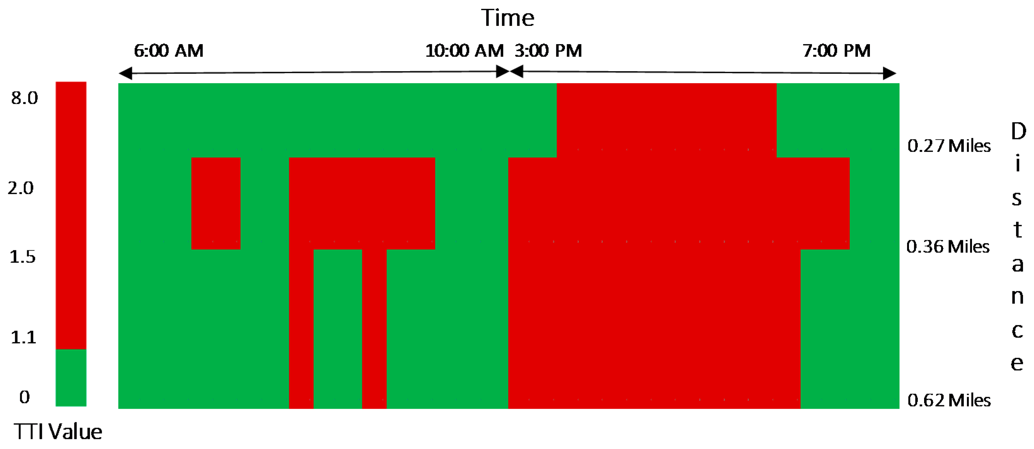
Congestion Intensity is a two-dimensional measure which accounts for the percentage of congested area in the time–space map [18]. Any time–space map includes two dimensions, i.e., the temporal dimension which is the study period (i.e., 6:00 a.m. to 10:00 a.m. and 3:00 p.m. to 7:00 p.m.), and the spatial dimension which is the length of TMCs along with selected segment. For illustration purposes, Figure 3 shows a sample of a time–space map developed for study segment 1. Each cell depicted on the map represents the TTI value. The associated range of color that reflects the level of congestion is set by defining different threshold values for TTI as shown on the left-hand side of Figure 3.
Figure 4 shows an example of the congested area (over space and time) which encompasses all cells with the TTI value of greater than 1.1.
Generating time–space maps in this study provided the information needed to calculate the daily percentage of Congestion Intensity. As shown in Equation (2), Congestion Intensity is the ratio between the congested area over the total area. The congested area represents the sum of the daily duration of congestion during AM and PM peak for each TMC multiplied to the length of the corresponding TMC. It is:
where:
- i: segment code
- j: work day
- n: TMC number along with segment i
- DOC: Duration of Congestion in minutes
- Time: Study period (6:00 a.m. to 10:00 a.m. and 3:00 p.m. to 7:00 p.m.) in minutes
The Congestion Intensity values for all workdays in 2015 ranged between 0% to 100%. These values can be utilized to calculate the 85th Percentile Congestion Intensity that adequately reflects the extent of congestion for the entire year. The 85th Percentile Congestion Intensity is a valuable metric that takes into account both the annual variability and reliability of congestion. The 85th Percentile of Congestion Intensity simply means that the Congestion Intensity has a lower value 85% of days.
3.2.4. Speed-Drop
Similar to Congestion Intensity, the Speed-drop is also a two-dimensional measure which accounts for the percentage of deviation from a Cutoff Speed in time-space map [18]. In the case of Speed-drop, each cell in the time–space map represents a reported speed, and when the speed value falls below the Cutoff Speed threshold, the cell is considered as a congested section. Cutoff Speed is the point where the TTI value equals to 1.1 and can be calculated from dividing the Free Flow Speed (FFS) by 1.1. The daily Speed-drop for each segment can be computed by utilizing Equation (3). This equation first calculates the percentage of deviation from Cutoff Speed (meaning the difference between the congested speed and the Cutoff speed as a percentage) for each cell. Then, the weighting factor is applied to each cell to obtain a weighted mean among all congested cells.
where:
- i: segment code
- j: work day
- m: cell inside the space-time map
- Cng SP: Congested Speed
- Cutoff SP: Cutoff Speed
- VMTm: Vehicle Mile Traveled for cell m, and
- VMT of Congested Area: Total Vehicle Mile Traveled in the congested area
In this study, instead of using VMT that requires having volume data, the weighting factor was calculated by applying the formula shown in Equation (4):
where:
- CellArea: Area for cell m that is equal to EPOCH x Length of TMC, and
- CongestedArea: Total congested area calculated according to the nominator in Equation (2).
In the Birmingham case study, calculating the Speed-drop for all workdays in 2015 provided a better understanding of the severity of congestion throughout the year. The resulting values werealso utilized to calculate the 85th Percentile of Speed-drop, which is another valuable metric related to congestion severity.
3.2.5. Impact Factor (IF)
Impact factor (IF) is a metric introduced in this study in order to capture the combined effect of both severity and extent of congestion throughout the year. It combines two measures, namely Congestion Intensity and Speed-drop, by multiplying their values for the corresponding day of the year and then computing the 85th percentile for the resulting values (Equation (5)). Developing Impact Factor is a robust method to identify segments that experience long-lasting and severe congestion throughout the year.
where:
- i: Segment code
- j: work day
4. Analysis and Results
4.1. Travel Time Index (TTI)
Based on the analysis of 2015 NPMRDS records for the 28 segments of the four Birmingham study corridors, TTI values were calculated and summarized in Table 2. Using the TTI threshold values as introduced in Section 3.2.1, Table 2 reveals the variability of travel time experienced by commuters using a color-coded scheme with the range of colors associated with the value of Travel Time Index. Green represents best and red represents worst conditions. The lower that the value of TTI is, the closer the travel condition is to free flow travel time.
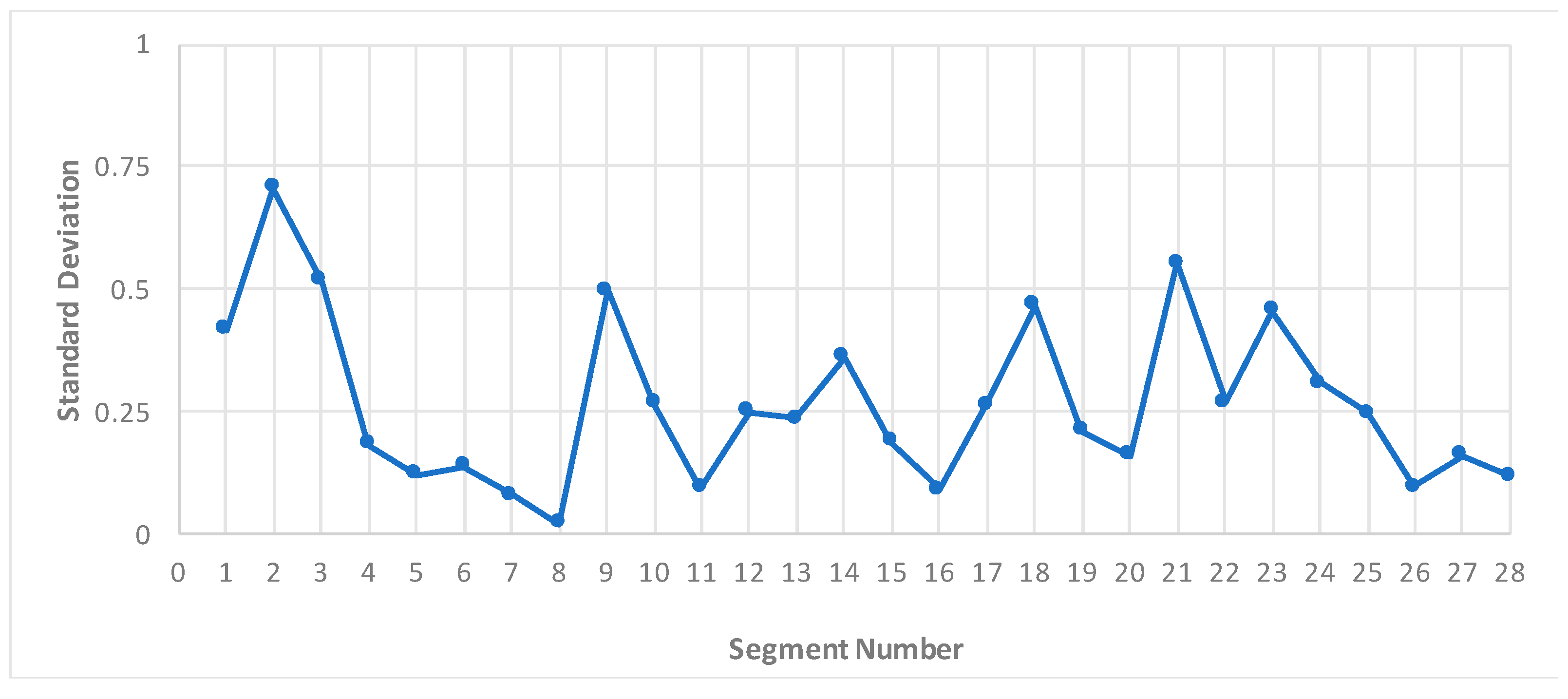
The standard deviation also was computed to help understand the variability of values during AM and PM peak periods (Figure 5). By considering the TTI values and associated standard deviations for each segment, conclusions can be drawn regarding the reliability of study segments. Given the results obtained for the Birmingham case study, it can be concluded that segment 8 is the most reliable segment in the study area as it displays the lowest values for TTI and standard deviation.
However, the highest values of TTI and standard deviation were obtained for segments 2 and 9. More specifically, the worst TTI value obtained was 4.91 for segment 2 under PM peak conditions in December. A TTI value of 4.91 means that the maximum average travel time during PM in the month of December in this segment was almost five times greater than the free flow travel time.
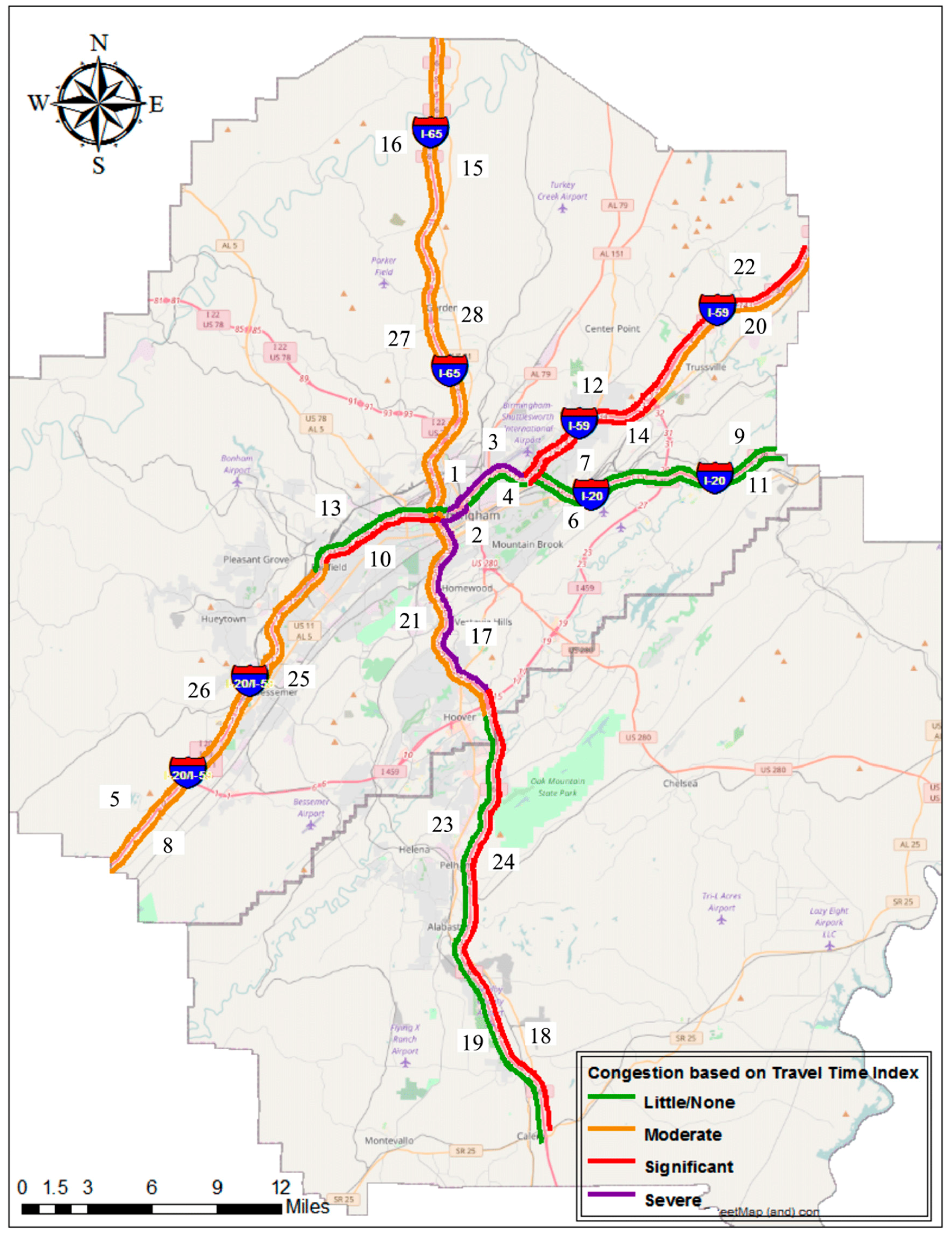
Furthermore, visual maps were developed by GIS software and used to display the congestion location, and severity along the study corridors. For demonstration purposes, Figure 6 and Figure 7 show the TTI values for January 2015 during AM peak and PM peak periods where segments shown as green, orange, red, and purple indicate “Little/None”, “Moderate”, “Significant”, and “Severe” congestion levels, respectively.
Close inspection of the results of the analysis shows that the level of congestion on study segments that provide primary access to the Birmingham downtown area highly depends on the time of day. For instance, I65 segments 17 and 21 carry travelers to/from the Birmingham downtown area during their commute. Segment 17 represents the northbound and segment 21 the southbound direction. As shown in Figure 6, during the AM peak, severe congestion occurred on segment 17 that carries commuters toward the downtown whereas segment 21 showed the moderate congestion. During the PM peak, the most significant congestion occurred in the opposite direction along segment 21 that travels from the downtown and outwards (Figure 7).
4.2. Duration of Congestion (DOC)
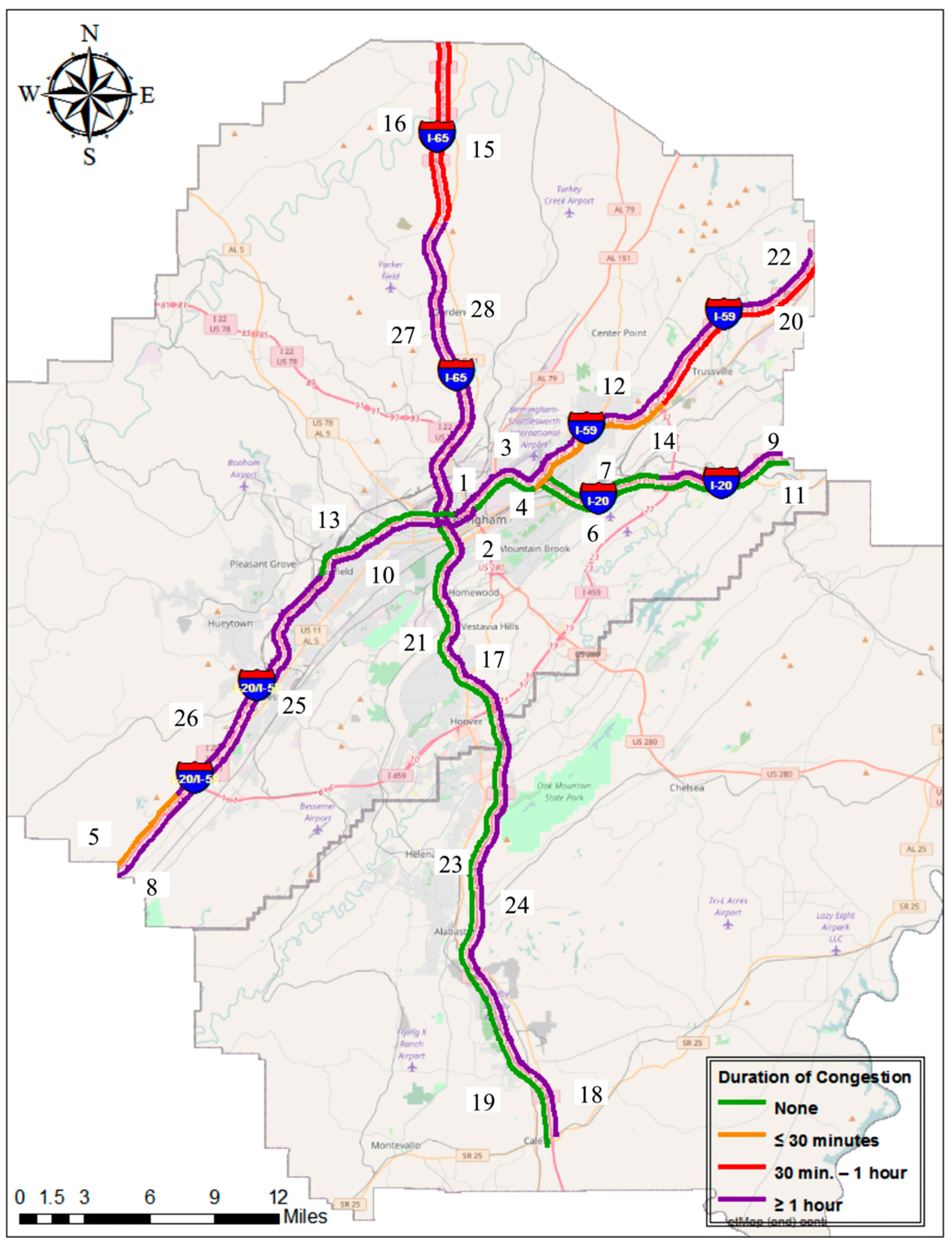
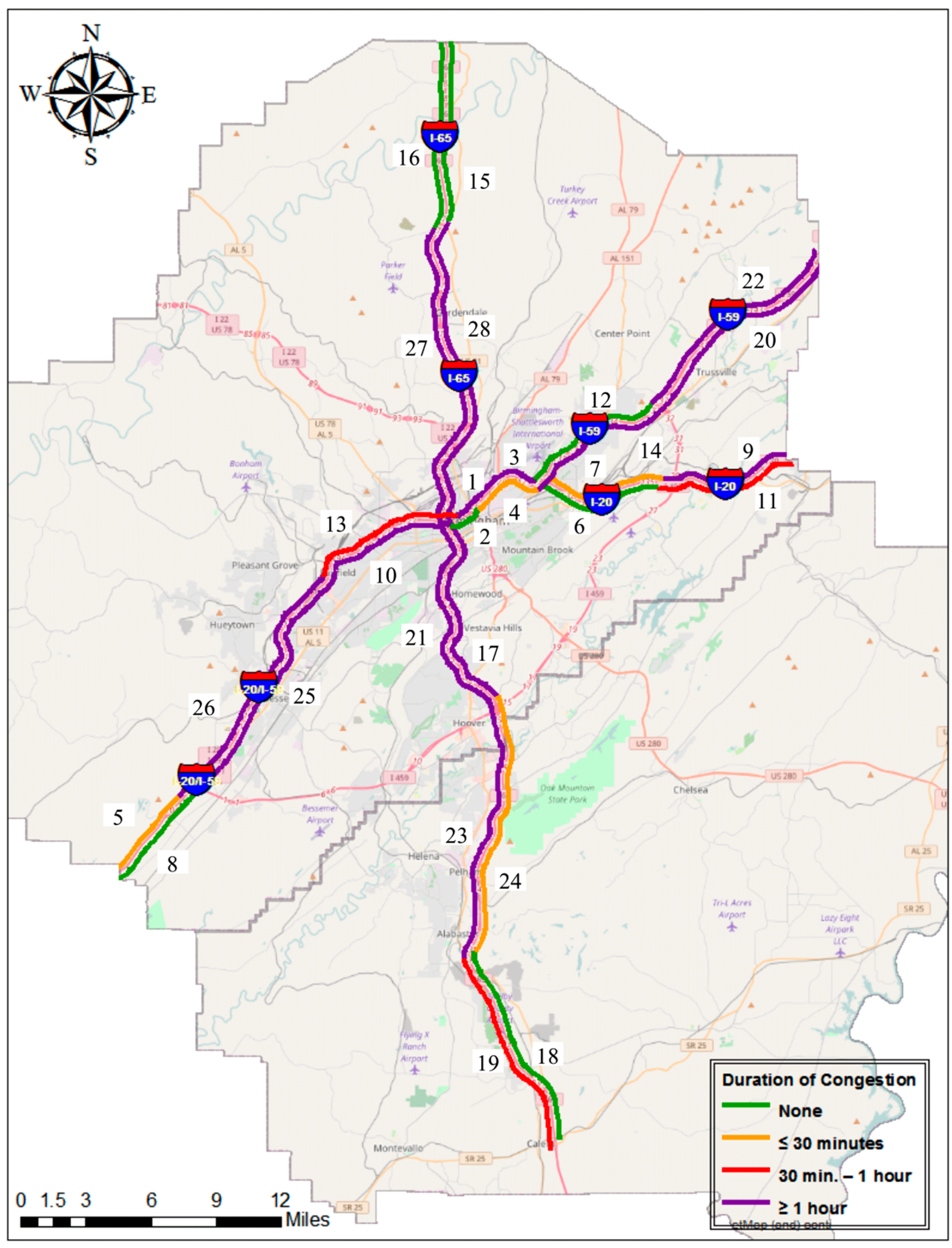
TTI values were used to calculate the Duration of Congestion (DOC) as defined in Section 3.2.2. The results for all study segments and for all 12 months considered were summarized in Table 3. Also, Figure 8 and Figure 9 were developed to help visualize the DOC on the study corridors during the AM and PM peak periods in January 2015.
It can be seen that congestion is persistent, continuing for more than 1 h during the peak periods. It should be noted that a high value for TTI does not necessary accompany a high value for congestion duration, since the DOC represents the persistence of congestion during peak hours and TTI shows the worst congested 15 min during peak hours. For instance, as shown in Table 3, segment 20 with TTI around 1.2 is moderately congested during AM peak in September and October 2015 but the duration of congestion is 240 min. This implies that commuters using segment 20 any time from 6:00 a.m. to 10:00 a.m. should adjust their travel plans as travel is expected to take almost twice the amount of travel time compared to the ideal condition. However, segment 2 with TTI equal to 2.08 experienced severe congestion in January 2015 but with duration of 90 min.
4.3. 85th Percentile of Congestion Intensity and Speed-Drop
Congestion Intensity and Speed-drop represent annual measures that reflect the extent and severity of all circumstances occurring over the year respectively. Such performance measures are an effective way to represent both expected and unexpected circumstances over the year.
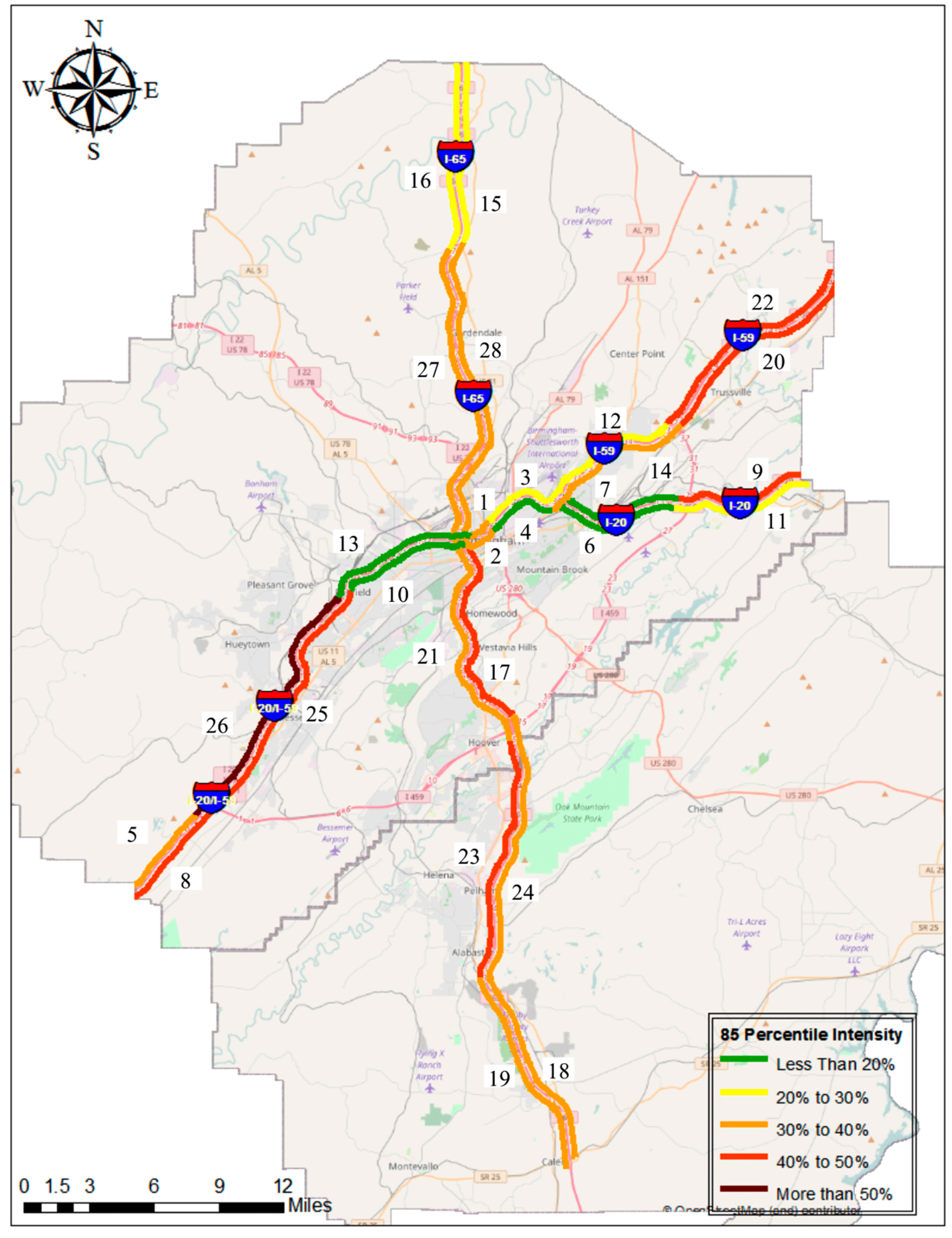
Table 4 shows the comparison among the 28 study segments based on their 85th Percentile Congestion Intensity and Speed-drop values, and Figure 10 and Figure 11 display their location in the study area. Inspection of the results displayed in Table 4 shows that segment 26 has the highest value in the 85th Percentile Congestion Intensity. This implies that during the AM and PM peak hours more than 50 percent of this segment is congested. However, segment 26 has a value of 6.31 percent for 85th Percentile Speed-drop which reveals that most of the area along this segment should be moderately congested. Though, segment 3 shows the highest value for 85th Percentile Speed-drop which suggests that a high level of delay occurs on this segment over the year. It can clearly be seen that a high value for 85th Percentile Congestion Intensity is not necessarily accompanied by a high value for 85th Percentile Speed-drop. Therefore, neither of these measures alone can be considered as an appropriate metric for ranking and prioritizing segments with respect to congestion mitigation needs.
4.4. Impact Factor
To compare and rank segments in a comprehensive way that captures the effect of both Congestion Intensity and Speed-drop, the Impact Factor was determined as defined in Section 3.2.5. The Impact Factor metric accounts for both reliability and variability of congestion throughout the year. Table 5 shows the Impact Factor for all study segments, ranked from the highest to the lowest value.
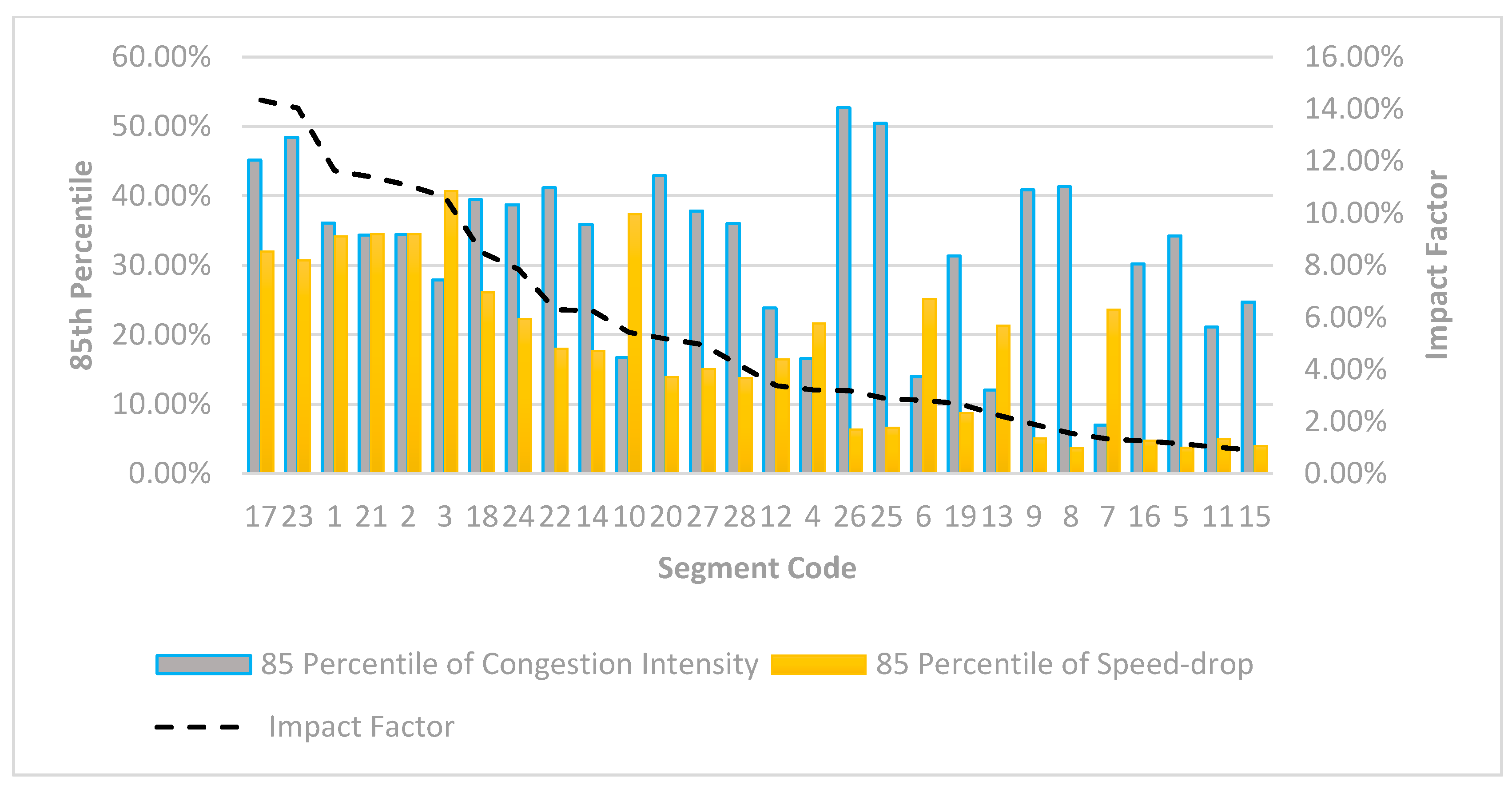
According to Table 5, study segments 17 and 23 with the highest values of Impact Factor are the least reliable segments and segments 15 and 11 with the lowest values are the most reliable study segments throughout the year 2015.
Figure 12 displays the Impact Factor values from highest to the lowest accompanied by the 85th Percentile of Congestion Intensity and Speed-drop for corresponding segments. It reveals that segments with the relatively high value for both 85th Percentile Congestion Intensity and Speed-drop result in a high Impact Factor as well.
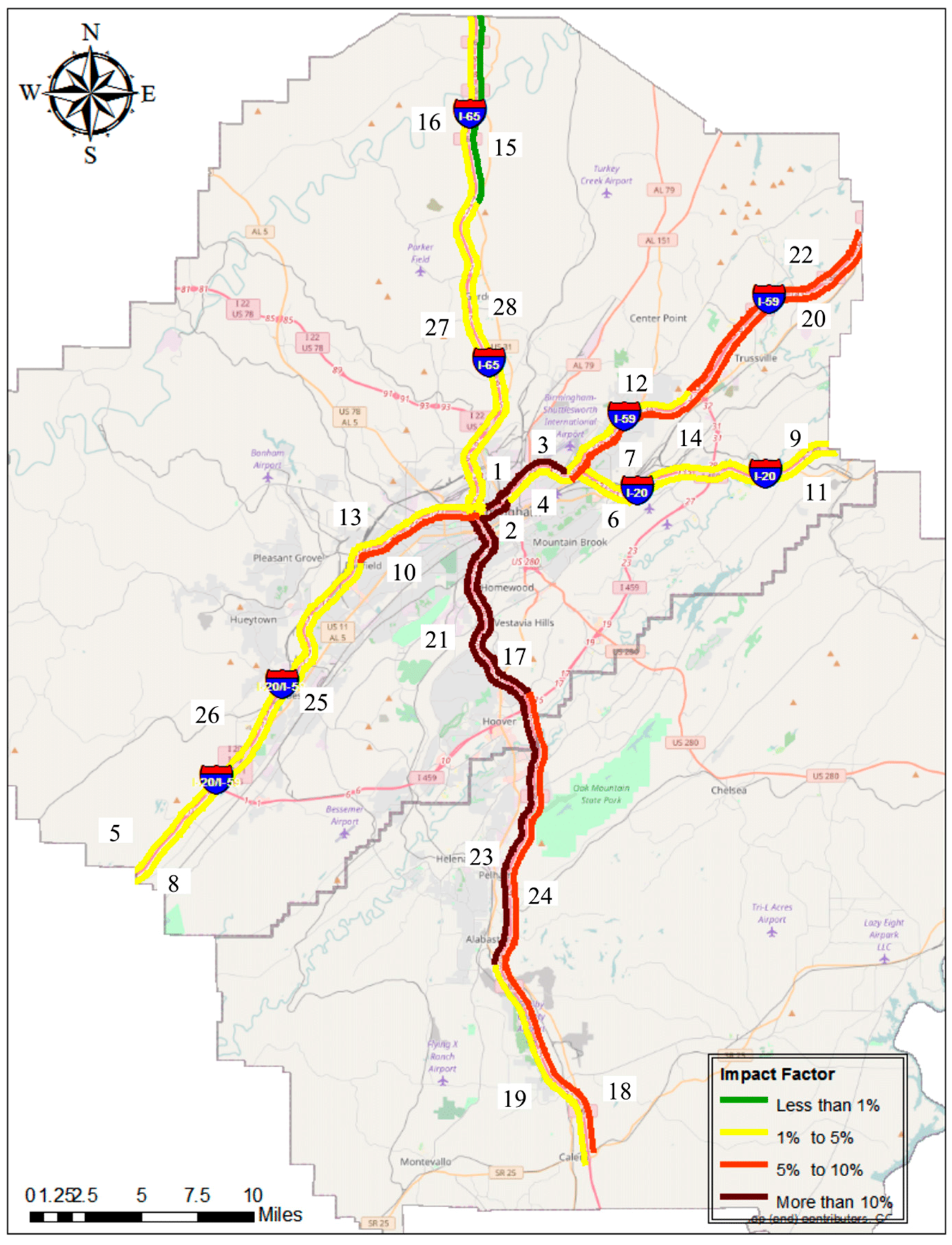
Figure 13 displays the location of study segments and their corresponding Impact Factor value and can help transportation officials and decision makers to determine high priority corridors for implementing strategies to address congestion. Review of Figure 13 indicates that part of I-65 located in the Southside of Birmingham (segments 17, 23, and 21) shows an impact factor higher than 10% and thus should be considered as of highest priority for receiving investment toward operational improvements.
5. Conclusions and Recommendations
This study was undertaken to (a) showcase the development of an automated process to facilitate the management, storage, and processing of big transportation data sets such as NPMRDS for congestion monitoring applications, (b) use traffic data analytics and statistical analysis to extract travel time reliability performance measures in a Birmingham case study, and (c) use reliability performance measures to determine the congestion extent and severity and guide optimization of traffic operations in the Birmingham region.
The case study utilized the NPMRDS data set in order to quantify congestion in the Birmingham region over an one-year period (2015) along four major freeways namely I-65, I-20, I-59, and I-20/I-59. RDBMS was employed as an efficient and economical tool for data management and SQL was used to extract data and perform the analysis. A range of performance measures was calculated for quantifying the congestion location, level, and extent, and used to prioritize freeway segments needs with respect to congestion. The performance measures calculated were the Travel Time Index (TTI), the Duration of Congestion (DOC), the 85th Percentile Congestion Intensity, and the 85th Speed-drop. In addition, calculation of an Impact Factor was proposed and used for ranking the congested segments. Such rankings can be used as a systematic and data-driven method for prioritizing resource allocations for operational improvements. The analysis revealed that the segments 17 and 23, with relatively high values for 85th Percentile Congestion Intensity and Speed-drop are the most unreliable segments in the study area and thus require close attention.
Overall, the study findings can be valuable in guiding transportation professionals and agencies on how to use big transportation databases such as NPMRDS to quantify the level and extent of congestion, and generate performance-based measures. Such performance measures can, in turn, be used as an initial screening process for congestion management purposes and help to identify locations where implementation of congestion mitigation initiatives have the best potential return for the investment.
Future work can consist of validating the proposed approach using a larger sample size. In addition, it is recommended that further studies be conducted that investigate in greater depth the effect of outliers on Travel Time Reliability measures. It is also desirable to extend the work to include consideration of additional data sources such as volume data, incident data, weather events and work zone presence information in order to improve the understanding of the causes of uncertainty in travel time and more accurately quantify recurrent and non-recurrent congestion in the future.
Acknowledgments
Funding for this study was provided by the Regional Planning Commission of Greater Birmingham Region. The support of the study sponsors is greatly appreciated. The authors also wish to acknowledge the valuable contributions of A. Sullivan and O. Ramadan to the study.
Author Contributions
S.H.R. participated in the research design, data analysis and interpretation, and prepared the manuscript. V.S. participated in the research design, results interpretation, and reviewed the manuscript. All authors read and approved the final manuscript.
Conflicts of Interest
The authors declare no conflicts of interest.
References
- Schrank, D.; Eisele, B.; Lomax, T. Urban Mobility Report; Texas A&M Transportation Institute: College Station, TX, USA, 2015. [Google Scholar]
- Gharaibeh, N.; Zwahlen, T.M. NCHRP Synthesis 508: Data Management and Governance Practices; N.A.O. Sciences: Buckingham, UK, 2017. [Google Scholar]
- Lomax, T.; Turner, S.; Shunk, G. NCHRP, R. 398: Quantifying Congestion; Transportation Research Board: Washington, DC, USA, 1997. [Google Scholar]
- Introduction to the National Performance Management Research Data Set (NPMRDS); HERE and the Volpe Center: Cambridge, MA, USA, 2013.
- Rafferty, P.; Hankley, C. Applying National Probe Data for Performance Measures: Crafting and Visualizing Mobility from the NPMRDS; Wisconsin Traffic Operations and Safety Laboratory: Madison, WI, USA, 2014. [Google Scholar]
- Liao, C.-F. Using Truck GPS Data for Freight Performance Analysis in the Twin Cities Metro Area; Minnesota Department of Transportation Research Services & Library, Department of Civil Engineering University of Minnesota: Minneapolis, MN, USA, 2014. [Google Scholar]
- Torrey, W.F. Cost of Congestion to the Trucking Industry; American Transportation Research Institute (ATRI): Arlington, VA, USA, 2014. [Google Scholar]
- Schoener, G. I-95 Corridor Coalition Probe Data Comparison; UMD CATT Lab: College Park, MD, USA, 2014; Available online: http://i95coalition.org/ (accessed on 25 November 2017).
- Travel Time Reliability Reference Manual. 2014. Available online: https://en.wikibooks.org/wiki/Travel_Time_Reliability_Reference_Manual/INRIX_Data_Types (accessed on 25 November 2017).
- The iPeMS MAP-21 Module: Producing the Information You Need from the National Performance Management Research Data Set (NPMRDS); ITERIS Inc.: Santa Ana, CA, USA, 2015.
- Federal Highway Administration (FHWA). 2015 Urban Congestion Trends: Communicating Improved Operations with Big Data; Federal Highway Administration: Washington, DC, USA, 2016.
- Nam, D.; Park, D.; Khamkongkhun, A. Estimation of value of travel time reliability. J. Adv. Transp. 2005, 39, 39–61. [Google Scholar] [CrossRef]
- Bell, M.G.H.; Iida, Y. The Network Reliability of Transport. In Proceedings of the 1st International Symposium on Transportation Network Reliability (INSTR), Kyoto, Japan, 31 July–1 August 2001; Pergamon Press: Oxford, UK, 2003. [Google Scholar]
- Lomax, T.; Schrank, D.; Turner, S. Selecting Travel Reliability Measures; Texas Transportation Institute: College Station, TX, USA, 2003. [Google Scholar]
- National Academies of Sciences, Engineering, and Medicine. Cost-Effective Performance Measures for Travel Time Delay, Variation, and Reliability; The National Academies Press: Washington, DC, USA, 2008. [Google Scholar]
- Tu, H.; Lint, J.W.V.; Zuylen, H.J.V. Travel Time Reliability Model on Freeways. In Proceedings of the 87th Annual Meeting of Transportation Research Board, Washington, DC, USA, 13–17 January 2008. [Google Scholar]
- Federal Highway Administration (FHWA). Travel Time Reliability: Making It There on Time; All the Time; U.S. Department of Transportation: Washington, DC, USA, 2006.
- Federal Highway Administration (FHWA). Traffic Bottlenecks: Identification and Solutions; FHWA: Washington, DC, USA, 2016.
Figure 1.
Case Study Freeway Network.
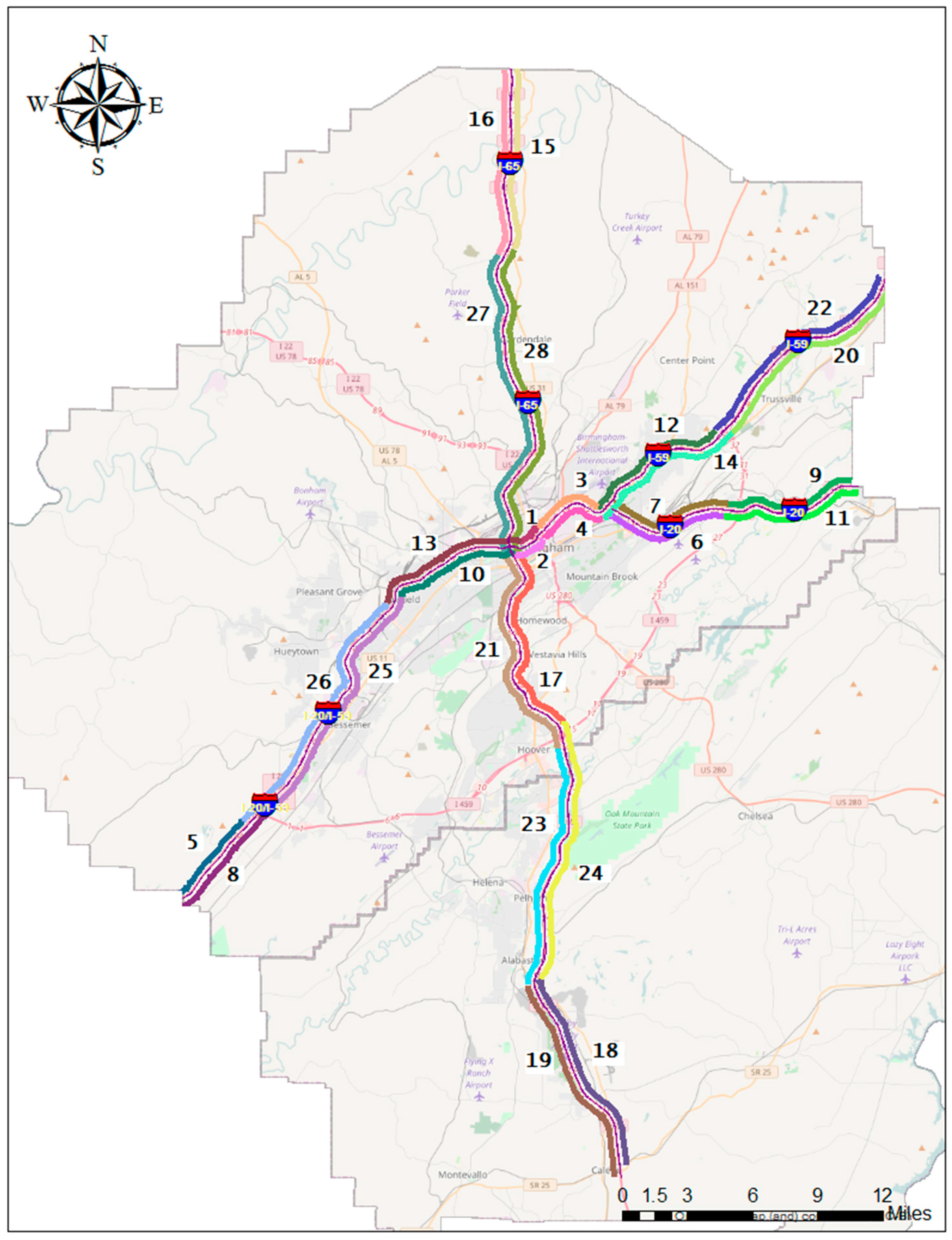
Figure 2.
Relationships and Primary Keys.
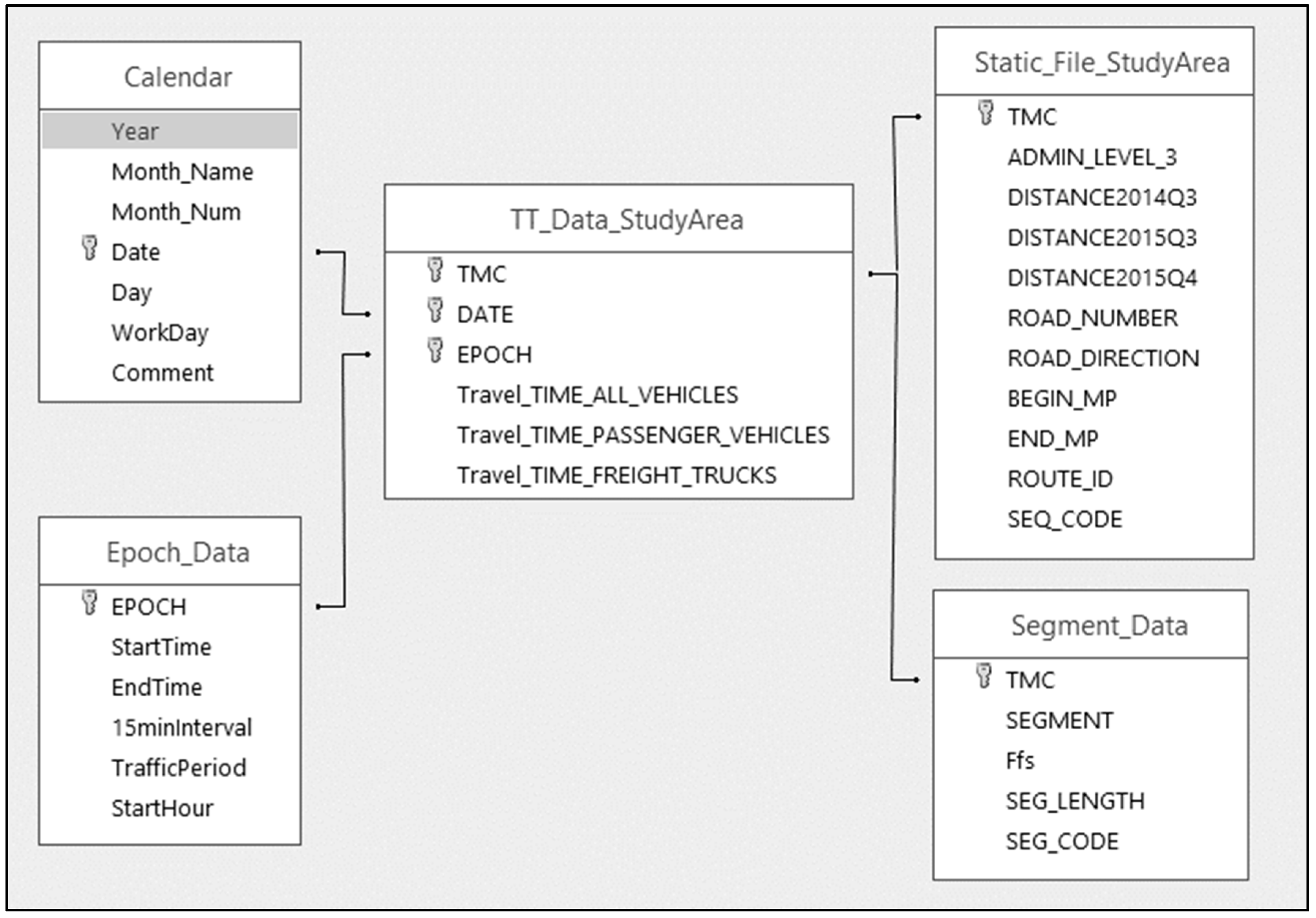
Figure 3.
Sample Time-Space Map.
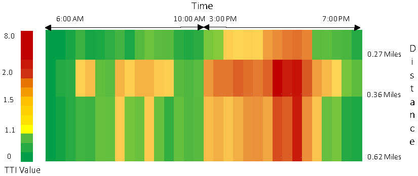
Figure 4.
Congested Area.

Figure 5.
Standard Deviation of TTI by Segment in 2015.

Figure 6.
Congestion Severity based on TTI during AM Peak, January 2015.

Figure 7.
Congestion Severity based on TTI during PM Peak, January 2015.
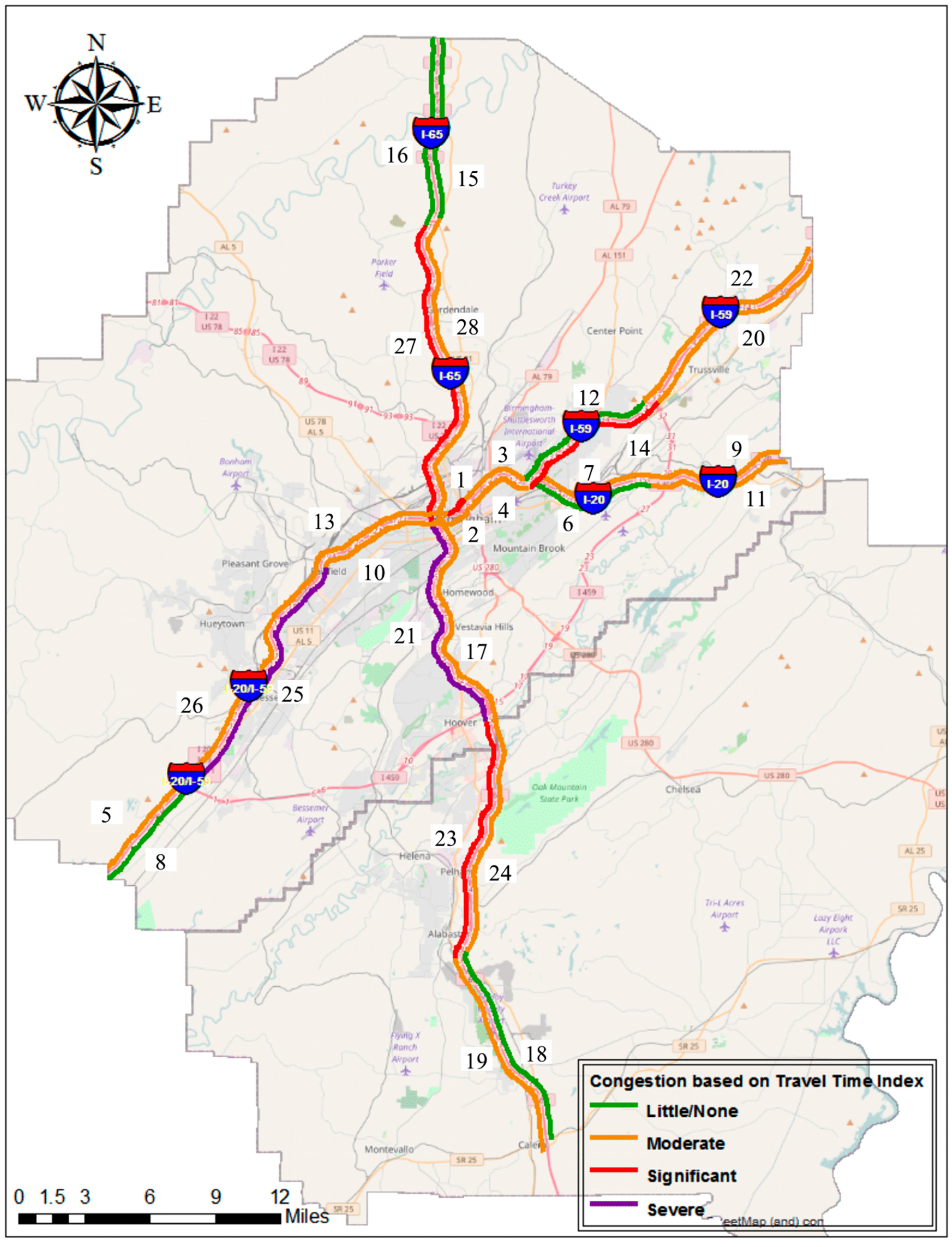
Figure 8.
Duration of Congestion during AM Peak in January 2015.

Figure 9.
Duration of Congestion during PM Peak in January 2015.

Figure 10.
85th Percentile Congestion Intensity in 2015.

Figure 11.
85th Percentile Speed-drop in 2015.
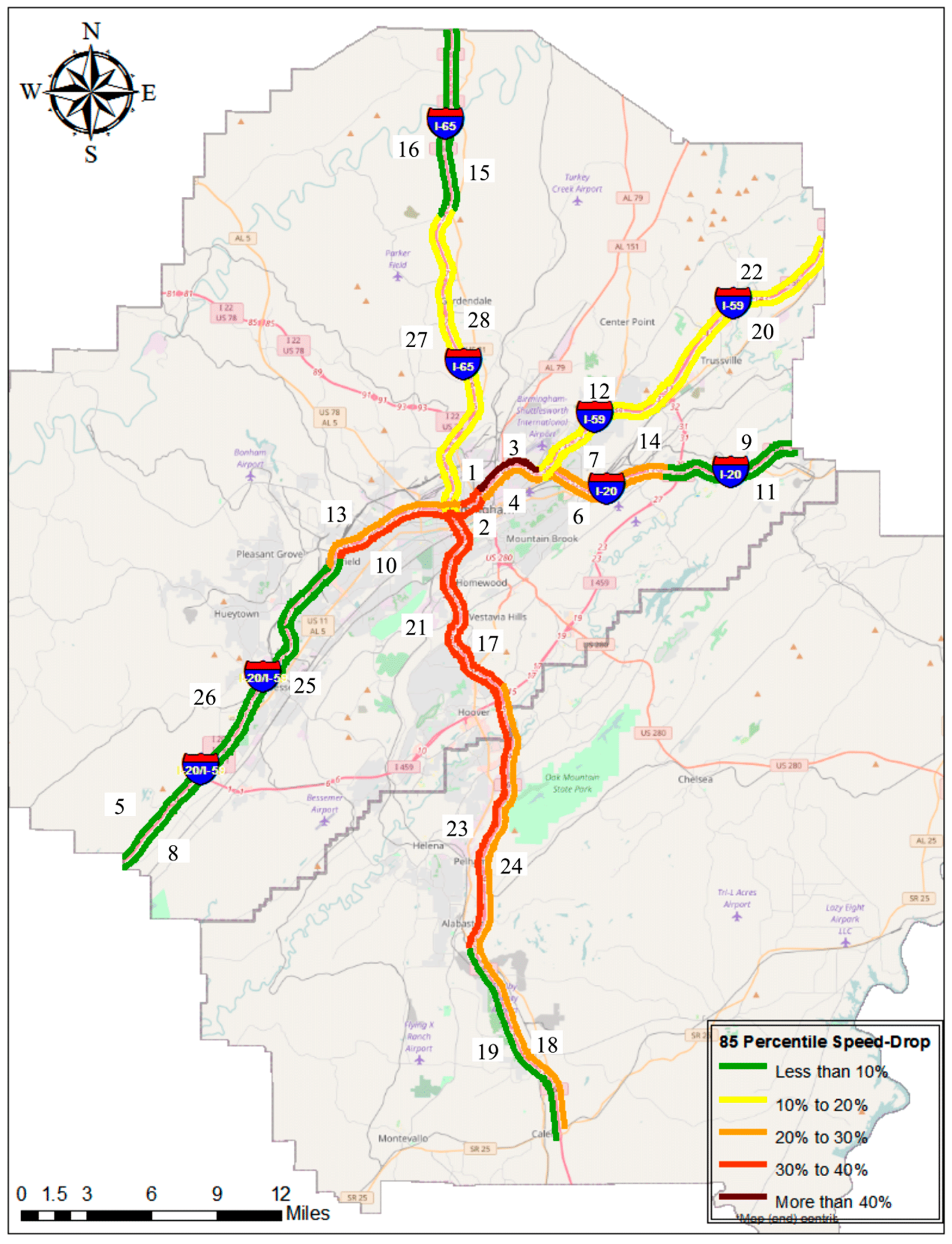
Figure 12.
Impact Factor along with 85th Percentile of Congestion Intensity and Speed-drop for all Study Segments in 2015.
Figure 12.
Impact Factor along with 85th Percentile of Congestion Intensity and Speed-drop for all Study Segments in 2015.

Figure 13.
Impact Factor for all Study Segments in 2015.


Table 1.
Study Segment Attributes.
| Road Number | Segment Name | Travel Direction | Segment Code | TMC Count | Length (mile) |
|---|---|---|---|---|---|
| I-20 | I20/59 to I459 | Eastbound | 6 | 6 | 5.87 |
| Westbound | 7 | 6 | 5.96 | ||
| I459 to St. Clair County | Eastbound | 11 | 3 | 6.65 | |
| Westbound | 9 | 3 | 6.43 | ||
| I-20/I-59 | I459 to Valley Road | Eastbound | 25 | 6 | 12.09 |
| Westbound | 26 | 6 | 12.74 | ||
| I65 to RME | Eastbound | 2 | 3 | 1.39 | |
| Westbound | 1 | 3 | 1.27 | ||
| RME to I20/59 Split | Eastbound | 4 | 4 | 3.44 | |
| Westbound | 3 | 4 | 3.34 | ||
| Tuscaloosa Co. Line to I459 | Eastbound | 8 | 2 | 5.98 | |
| Westbound | 5 | 3 | 6.54 | ||
| Valley Road to I65 | Eastbound | 10 | 8 | 7.04 | |
| Westbound | 13 | 9 | 7.76 | ||
| I-59 | I20/59 to I459 | Northbound | 14 | 7 | 7.76 |
| Southbound | 12 | 6 | 7.47 | ||
| I459 to St. Clair County | Northbound | 20 | 4 | 10.45 | |
| Southbound | 22 | 5 | 10.85 | ||
| I-65 | Chilton County Line to US31 in Alabaster | Northbound | 18 | 3 | 9.99 |
| Southbound | 19 | 3 | 10.04 | ||
| I20/59 to US31/Mary Buckelew | Northbound | 28 | 10 | 15.10 | |
| Southbound | 27 | 9 | 14.42 | ||
| I459 to I20/59 | Northbound | 17 | 10 | 9.44 | |
| Southbound | 21 | 11 | 10.69 | ||
| US31 (Exit 275) to Cullman County Line | Northbound | 15 | 8 | 13.96 | |
| Southbound | 16 | 9 | 16.65 | ||
| US31 in Alabaster to I459 | Northbound | 24 | 6 | 12.53 | |
| Southbound | 23 | 6 | 11.83 |
Table 2.
Max Time Travel Index (TTI) Values during AM Peak by Month in 2015.

Table 3.
Congestion Duration during Peak Periods in 2015.

Table 4.
Segments 85th Percentile Congestion Intensity and Speed-drop.
| Segment Code | 85 Percentile of intensity | 85 Percentile of Speed Drop |
|---|---|---|
| 26 | 52.67% | 6.31% |
| 25 | 50.44% | 6.62% |
| 23 | 48.40% | 30.70% |
| 17 | 45.15% | 31.99% |
| 20 | 42.92% | 13.86% |
| 8 | 41.30% | 3.66% |
| 22 | 41.15% | 17.96% |
| 9 | 40.88% | 5.04% |
| 18 | 39.43% | 26.10% |
| 24 | 38.74% | 22.28% |
| 27 | 37.84% | 15.02% |
| 1 | 36.12% | 34.17% |
| 28 | 36.06% | 13.73% |
| 14 | 35.87% | 17.67% |
| 2 | 34.43% | 34.51% |
| 21 | 34.36% | 34.52% |
| 5 | 34.26% | 3.74% |
| 19 | 31.33% | 8.73% |
| 16 | 30.19% | 4.74% |
| 3 | 27.88% | 40.67% |
| 15 | 24.71% | 4.00% |
| 12 | 23.84% | 16.42% |
| 11 | 21.12% | 4.99% |
| 10 | 16.68% | 37.35% |
| 4 | 16.56% | 21.65% |
| 6 | 13.97% | 25.17% |
| 13 | 12.04% | 21.31% |
| 7 | 7.00% | 23.63% |
Table 5.
Segments Impact Factors in 2015.
| Segment Code | |
|---|---|
| 23 | 14.85% |
| 17 | 14.44% |
| 1 | 12.34% |
| 2 | 11.88% |
| 21 | 11.86% |
| 3 | 11.34% |
| 18 | 10.29% |
| 24 | 8.63% |
| 22 | 7.39% |
| 14 | 6.34% |
| 10 | 6.23% |
| 20 | 5.95% |
| 27 | 5.68% |
| 28 | 4.95% |
| 12 | 3.92% |
| 4 | 3.59% |
| 6 | 3.51% |
| 25 | 3.34% |
| 26 | 3.32% |
| 19 | 2.74% |
| 13 | 2.57% |
| 9 | 2.06% |
| 7 | 1.65% |
| 8 | 1.51% |
| 16 | 1.43% |
| 5 | 1.28% |
| 11 | 1.05% |
| 15 | 0.99% |
© 2017 by the authors. Licensee MDPI, Basel, Switzerland. This article is an open access article distributed under the terms and conditions of the Creative Commons Attribution (CC BY) license (http://creativecommons.org/licenses/by/4.0/).
Share and Cite
MDPI and ACS Style
Sisiopiku, V.P.; Rostami-Hosuri, S. Congestion Quantification Using the National Performance Management Research Data Set. Data 2017, 2, 39. https://doi.org/10.3390/data2040039
AMA Style
Sisiopiku VP, Rostami-Hosuri S. Congestion Quantification Using the National Performance Management Research Data Set. Data. 2017; 2(4):39. https://doi.org/10.3390/data2040039
Chicago/Turabian StyleSisiopiku, Virginia P., and Shaghayegh Rostami-Hosuri. 2017. "Congestion Quantification Using the National Performance Management Research Data Set" Data 2, no. 4: 39. https://doi.org/10.3390/data2040039