Real-Time Fuzzy Data Processing Based on a Computational Library of Analytic Models

Abstract

This work focuses on fuzzy data processing in control and decision-making systems based on the transformation of real-timeseries and high-frequency data to fuzzy sets with further implementation of diverse fuzzy arithmetic operations. Special attention was paid to the synthesis of the computational library of horizontal and vertical analytic models for fuzzy sets as the results of fuzzy arithmetic operations. The usage of the developed computational library allows increasing the operating speed and accuracy of fuzzy data processing in real time. A computational library was formed for computing of such fuzzy arithmetic operations as fuzzy-maximum. Fuzzy sets as components of fuzzy data processing were chosen as triangular fuzzy numbers. The analytic models were developed based on the analysis of the intersection points between left and right branches of considered triangular fuzzy numbers with different relations between their parameters. Our study introduces the mask for the evaluation of the relations between corresponding parameters of fuzzy numbers that allows to determine the appropriate model from the computational library in automatic mode. The simulation results confirm the efficiency of the proposed computational library for different applications.

1. Introduction

Increasing the efficiency of the real-time control systems and decision-making processes under uncertain conditions deals with creating new techniques for Big Data processing, management, and analysis taking into account the dynamic nature of real objects’ signals and information [1,2,3].

To this day, there are some successful mathematical methods, algorithms, and approaches developed based on the theory of computational intelligence, machine learning, soft computing, and recent advancements in cognitive computing [4,5,6,7]. Nevertheless, the exponential growth of the volume of modern Big Data and increasing velocity of their formation requires constant improvement and modifications of such methods. Special attention should be paid to the application of the theory of fuzzy sets, fuzzy logic, and fuzzy optimization as powerful tools for Big Data analysis and processing in terms of solving real-world problems in uncertain or fuzzy conditions [8,9,10]. As the fuzzy sets theory was primarily introduced in the publication by L. Zadeh [11], a lot of world-class scientists devoted their research to the field of fuzzy logic and its application in control, decision-making, and signal processing for investigation of various complex systems in engineering, economics, management, and so on [5,8,12,13].

Recent publications reveal how various fuzzy and other intelligent algorithms can be realized by computers and other different computing means for embedded signal processing, decision-making, and control systems. In particular, different algorithms of fuzzy control strategies in the embedded control systems with specific architectures can be successfully implemented based on such electronic devices as PLCs (Programmable Logic Controllers) [14,15,16,17,18] and reconfigurable FPGA (Field Programmable Gate Array) systems [19,20,21]. Moreover, a lot of advantages are in applications of the microcontroller Arduino [22,23,24] and the microprocessor Raspberry Pi [25,26] for the real-time fuzzy data computations and fuzzy information processing in diverse applications.

The necessity to solve different serious tasks in uncertain data analysis, as well as new requirements (e.g., reducing time and computational complexity) for real-time Big Data processing serve as a motivation for the development of new fuzzy techniques, models, and algorithms that increase efficiency (e.g., computation speed, accuracy, reliability, dependability, etc.) [1,3,5,9,27] of applied problems solving [1,2,5,28].

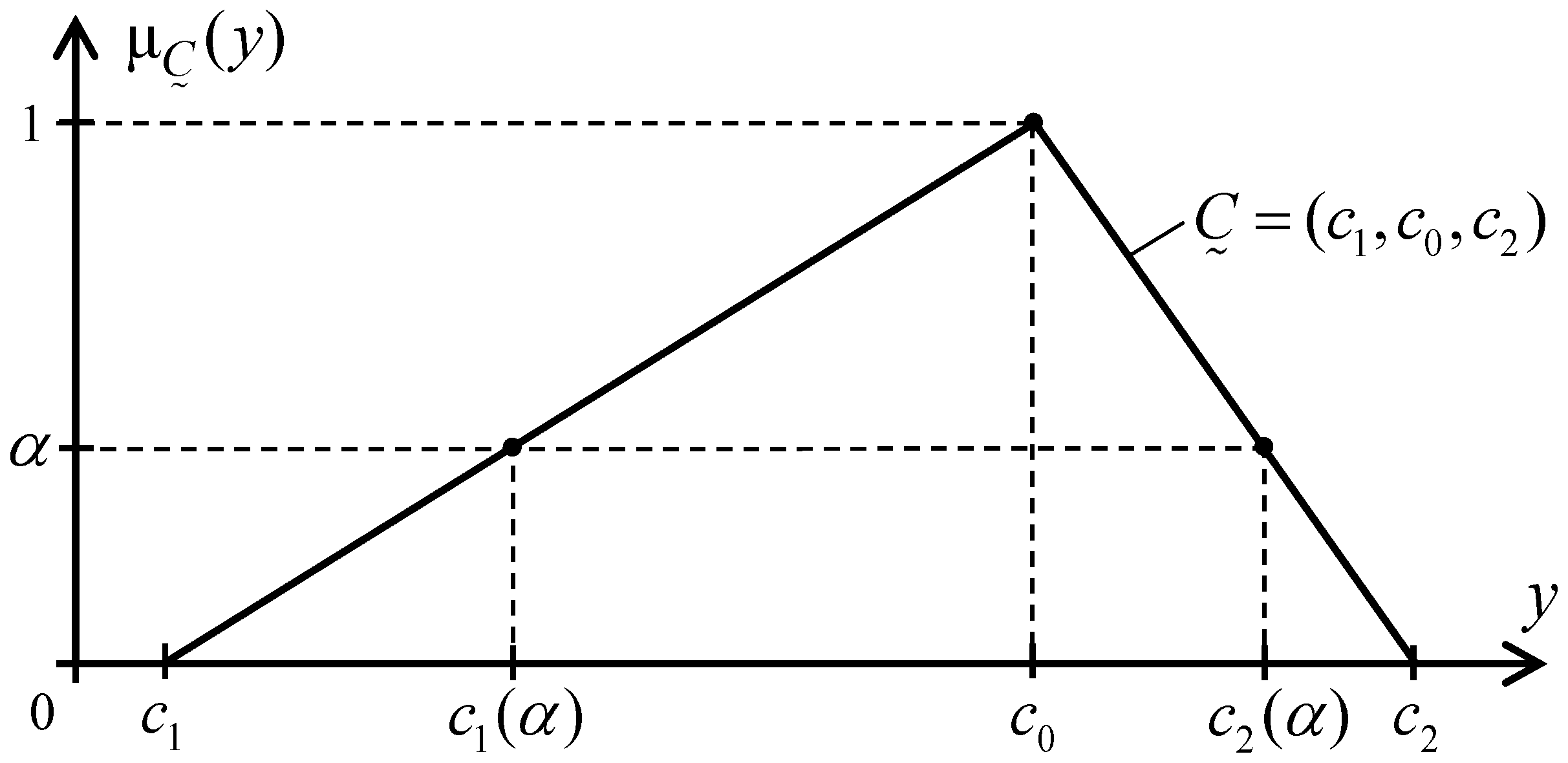
We will consider a fuzzy set $\underset{˜}{C}$ (Figure 1) as a set of couples $\left(y,{\mu }_{\underset{˜}{C}}\left(y\right)\right)$, where $y$ is an element on the universal set $U$ [11,29,30] which belongs to the fuzzy set $\underset{˜}{C}$ with a corresponding degree of confidence or the specific membership function (MF) value ${\mu }_{\underset{˜}{C}}\left(y\right)\in \left[0,1\right]$.

Successful examples of fuzzy technique application for finding efficient solutions under uncertainty in various fields of human activity include automation of the different technological processes, optimization of transport routes and logistics planning, evaluation of the investment and perspective research project proposals, decision making in medical diagnostics and medical image retrieval, management of banking and finances, etc. These techniques for data analysis rely, for example, on the usage of such flexible soft computing components as (a) non-parametrized and parametrized operators of t-norm and s-norm [29], t-concepts [31], fuzzy signatures and signatures trees [32], vector quantization and fuzzy S-tree [33], (b) different fuzzy inference engines (Mamdani, Sugeno, etc. [13,29]), (c) as well as different fuzzy approaches for implementation of fuzzy arithmetic operations with fuzzy numbers (FNs), including FNs-minimum, FNs-maximum, FNs-subtraction, FNs-multiplication, FNs-division, and FNs-addition [29,30,34,35,36,37,38,39].

Special attention should be paid to the formation of the resulting analytic models for fuzzy arithmetic because of their capacity to increase the accuracy and speed of the Big Data processing [30,34]. In some practical cases, it is possible to transform the big volume of information to corresponding fuzzy numbers [29,40] with further implementation of the resulting MFs for corresponding arithmetic operations with FNs.

One of the efficient approaches for the synthesis of the resulting MFs’ analytic models is using $\alpha$-cuts [29,34,41], in particular, for construction of the horizontal (inverse) and vertical (direct) models of the resulting membership functions. However, in some cases, the necessity to form such resulting models is time consuming and leads to the decrease in data processing speed and lower quality of the real-time control and decision-making processes [1,34,42,43].

Another approach deals with usage of Zadeh’s extension principle [29,43,44,45] or algorithm of Max-Min convolution [30], which requires a transformation of each initial fuzzy set (involved in fuzzy data processing) to discrete form using a discreteness step $\Delta y=\frac{y_{\max }-y_{\min }}{K}=const$ for determining $y_{i+1}=y_i+\Delta y,\left(i=0,1,2,\dots ,K\right)$. This leads to the synthesis of the resulting fuzzy sets, for example $\underset{˜}{S}$, in the table style or as a set of united singletons $\underset{˜}{S}={\displaystyle \sum _{i=0}^K\frac{{\mu }_{\underset{˜}{S}}\left(y_i\right)}{y_i}}$.

The abovementioned $\alpha$-cuts and Max-Min convolution approaches [29,30] require additional mathematical transformations for obtaining an analytic model of membership function ${\mu }_{\underset{˜}{S}}\left(y\right)$ of the resulting fuzzy set $\underset{˜}{S}$ which can be used for computing (for any $y^{\ast },y^{\ast }\in \left[y_{\min },y_{\max }\right]$) the corresponding membership’s value ${\mu }_{\underset{˜}{S}}\left(y^{\ast }\right)$ that characterizes belonging $y^{\ast }$ to the resulting fuzzy set $\underset{˜}{S}$. The mathematical formalization of the resulting analytic model ${\mu }_{\underset{˜}{S}}\left(y\right)$ can be realized based on the polynomial approximation [29] for the discrete fuzzy set $\underset{˜}{S}={\displaystyle \sum _{i=0}^K\frac{{\mu }_{\underset{˜}{S}}\left(y_i\right)}{y_i}}$. The usage of the interpolation procedure is also possible for calculation of the corresponding value ${\mu }_{\underset{˜}{S}}\left(y^{\ast }\right)$, in the case if $y^{\ast }$ is situated between any neighboring values $y_i$ and $y_{i+1}$, that is $y_i<y^{\ast }<y_{i+1}$. Both considered approaches are based on the implementation of the “multi-step” computational procedures. Any changes in the initial fuzzy sets requires implementing the polynomial approximation or interpolation procedures for fuzzy data processing that leads to the increase of computing complexity and computational time as well as decrease of the accuracy of calculations. Thus, the development of the new methods for automation of the procedures of resulting analytic models’ synthesis can significantly improve the quality of the “one-step” computational processes in fuzzy data processing.

This research aims to propose the advancements in the construction of the universal horizontal and vertical analytic models of the resulting MFs as main components of the generalized computational library that provide (a) automatic choice of the desired analytic models from the computational library based on the relationships between parameters of the initial fuzzy sets for fuzzy data processing and (b) improvement in the operating velocity and accuracy of the fuzzy arithmetic operations with special attention to FNs-maximum (maximum of fuzzy numbers) as one of the most difficult and complex (in computing aspects) arithmetic operations. This paper contributes to the literatures on fuzzy data processing and Big Data analysis [1,2,43].

The rest of the article is organized as follows. Main definitions and the problem statement may be found in Section 2. Section 3 describes the methodology of the analytic models’ synthesis for the results of the arithmetic operation FNs-maximum with triangular fuzzy numbers. All components of the developed computational library for different relations between FNs’ parameters as corresponding sets of the resulting horizontal and vertical models are presented in Section 4. Modelling results for validation of the synthesized analytic models, which were obtained with the usage of the corresponding masks and proposed computation library, are discussed in Section 5. Section 6 summarizes the article and suggests some directions for future research.

2. Problem Statement

Using $\alpha$-cuts for the implementation of FNs-maximum for two fuzzy sets leads to the step-by-step realization of the corresponding arithmetic algorithm for different $\alpha$-levels [29,30,34] (Figure 1):

$${\alpha }_i={\alpha }_{i-1}+\delta \alpha ,\left(i=1,2,\dots ,N\right)$$

(1)

where $\delta \alpha$ is a discreteness step, which can be calculated as $\delta \alpha =\frac{1}{N}$;

This iterative procedure has high computing complexity and the choice of the parameter $N$ and corresponding value $\delta \alpha$ sufficiently influences the computing velocity and calculation accuracy of the resulting MF [29,36,37].

In general, $\alpha$-cut $C_{\alpha }=\left\{y|{\mu }_{\underset{˜}{C}}\left(y\right)\ge \alpha \right\},$ $\alpha \in \left[0,1\right]$ of the fuzzy number $\underset{˜}{C}\in R$ is a crisp subset that includes (Figure 1) only values $y\in R$ with not less than $\alpha$ membership degree of belonging to the set $\underset{˜}{C}$, where $R$ is a set of real numbers [29,30]. For fuzzy sets $\underset{˜}{C}\in R,\underset{˜}{D}\in R$ it is possible to represent their $\alpha$-sets $C_{\alpha }$ and $D_{\alpha }$ in such style as:

$$C_{\alpha }=\left[c_1\left(\alpha \right),c_2\left(\alpha \right)\right],$$

(2)

$$D_{\alpha }=\left[d_1\left(\alpha \right),d_2\left(\alpha \right)\right],\alpha \in \left[0,1\right].$$

(3)

The computing of FNs-maximum will be more efficient in terms of the computational velocity and accuracy in the case of an analytic model of resulting MF that can be preliminarily synthesized [42]. The main goal of this study is the synthesis of the computational library of the resulting horizontal and vertical analytical models for the arithmetic operation of FNs-maximum in order to (a) decrease the complexity of the calculation process, (b) increase operating velocity of the arithmetic operation, (c) exclude the rooting iterative computing procedure, and (d) increase the accuracy of fuzzy data processing.

Let us present the synthesis procedure for abovementioned computational library [42,43] based on the MFs of triangular fuzzy numbers (TrFNs) with different relations $\mathbb{R}$ between their parameters (Figure 1).

The triangular fuzzy numbers $\underset{˜}{C}=\left(c_1,c_0,c_2\right)$ and $\underset{˜}{D}=\left(d_1,d_0,d_2\right)$ can be characterized by their own MFs ${\mu }_{\underset{˜}{C}}\left(y\right)$ and ${\mu }_{\underset{˜}{D}}\left(y\right)$ with corresponding parameters ${\mu }_{\underset{˜}{C}}\left(c_0\right)=1,$ ${\mu }_{\underset{˜}{D}}\left(d_0\right)=1,$ ${\mu }_{\underset{˜}{C}}\left(c_1\right)=0,$ ${\mu }_{\underset{˜}{C}}\left(c_2\right)=0,$ ${\mu }_{\underset{˜}{D}}\left(d_1\right)=0,$ and ${\mu }_{\underset{˜}{D}}\left(d_2\right)=0$. The horizontal $C_{\alpha },D_{\alpha }$ and vertical ${\mu }_{\underset{˜}{C}}\left(y\right)$, ${\mu }_{\underset{˜}{D}}\left(y\right)$ models of the triangular fuzzy numbers $\underset{˜}{C}\in R,\underset{˜}{D}\in R$ can be represented by the expressions (4)–(7) [29,30,34,35,36,37,42,43]:

$$C_{\alpha }=\left[c_1\left(\alpha \right),c_2\left(\alpha \right)\right]=\left[c_1+\alpha \left(c_0-c_1\right),c_2-\alpha \left(c_2-c_0\right)\right],$$

(4)

$${\mu }_{\underset{˜}{C}}\left(y\right)=\{\begin{array}{c}0,\forall \left(y\le c_1\right)\cup \left(y\ge c_2\right)\\ F_{C_L}\left(y,c_1,c_0\right),\forall \left(c_1<y\le c_0\right)\\ F_{C_R}\left(y,c_0,c_2\right),\forall \left(c_0<y<c_2\right)\end{array},$$

(5)

$$D_{\alpha }=\left[d_1\left(\alpha \right),d_2\left(\alpha \right)\right]=\left[d_1+\alpha \left(d_0-d_1\right),d_2-\alpha \left(d_2-d_0\right)\right],$$

(6)

$${\mu }_{\underset{˜}{D}}\left(y\right)=\{\begin{array}{c}0,\forall \left(y\le d_1\right)\cup \left(y\ge d_2\right)\\ F_{D_L}\left(y,d_1,d_0\right),\forall \left(d_1<y\le d_0\right)\\ F_{D_R}\left(y,d_0,d_2\right),\forall \left(d_0<y<d_2\right)\end{array},$$

(7)

where $F_{C_L}\left(y,c_1,c_0\right)=\left(y-c_1\right)/\left(c_0-c_1\right)$ is the left branch of the MF ${\mu }_{\underset{˜}{C}}\left(y\right)$ for TrFN $\underset{˜}{C}$; $F_{D_L}\left(y,d_1,d_0\right)=\left(y-d_1\right)/\left(d_0-d_1\right)$ is the left branch of the MF ${\mu }_{\underset{˜}{D}}\left(y\right)$ for TrFN $\underset{˜}{D}$; $F_{C_R}\left(y,c_0,c_2\right)=\left(c_2-y\right)/\left(c_2-c_0\right)$ is the right branch of the MF ${\mu }_{\underset{˜}{C}}\left(y\right)$ for TrFN $\underset{˜}{C}$; and $F_{D_R}\left(y,d_0,d_2\right)=\left(d_2-y\right)/\left(d_2-d_0\right)$ is the right branch of the MF ${\mu }_{\underset{˜}{D}}\left(y\right)$ for TrFN $\underset{˜}{D}$.

In the case of FNs-maximum computation, the usage of such algorithms as Max-Min or Min-Max convolutions [30,42], comparative to the $\alpha$-cuts algorithm, in many cases leads (a) to the violation of the properties of normality and convexity of the resulting fuzzy set $\underset{˜}{S}=\underset{˜}{C}(\vee )\underset{˜}{D}$ and (b) to the increasing complexity and calculation time for the fuzzy data processing.

Finally, the operation of FNs-maximum $\left(\underset{˜}{S}=\underset{˜}{C}(\vee )\underset{˜}{D}\right)$ can be presented using $\alpha$-cuts in such a style:

$$\begin{array}{cc}\hfill S_{\alpha }=C_{\alpha }(\vee )D_{\alpha }& =\left[c_1\left(\alpha \right),c_2\left(\alpha \right)\right](\vee )\left[d_1\left(\alpha \right),d_2\left(\alpha \right)\right]=\hfill \\ & =\left[c_1\left(\alpha \right)\vee d_1\left(\alpha \right),c_2\left(\alpha \right)\vee d_2\left(\alpha \right)\right],\hfill \end{array}$$

(8)

where $S_{\alpha }=\left[s_1\left(\alpha \right),s_2\left(\alpha \right)\right]$ is a horizontal model of the resulting fuzzy set $\underset{˜}{S}$. The functional parameters $\left\{c_1\left(\alpha \right),c_2\left(\alpha \right),d_1\left(\alpha \right),d_2\left(\alpha \right)\right\}$ of the horizontal models (4) and (6) will be used in Section 3 for transformation of the step-by-step $\alpha$-cuts procedure of the FNs-maximum processing (8) to synthesis of the universal analytic models of the resulting fuzzy set $\underset{˜}{S}=\underset{˜}{C}(\vee )\underset{˜}{D}$ for one-step computational procedure of the resulting membership function values ${\mu }_{\underset{˜}{S}}\left(y\right)$.

3. Formation of the Horizontal and Vertical Resulting Models for Fuzzy Arithmetic Operation “TrFNs-Maximum”

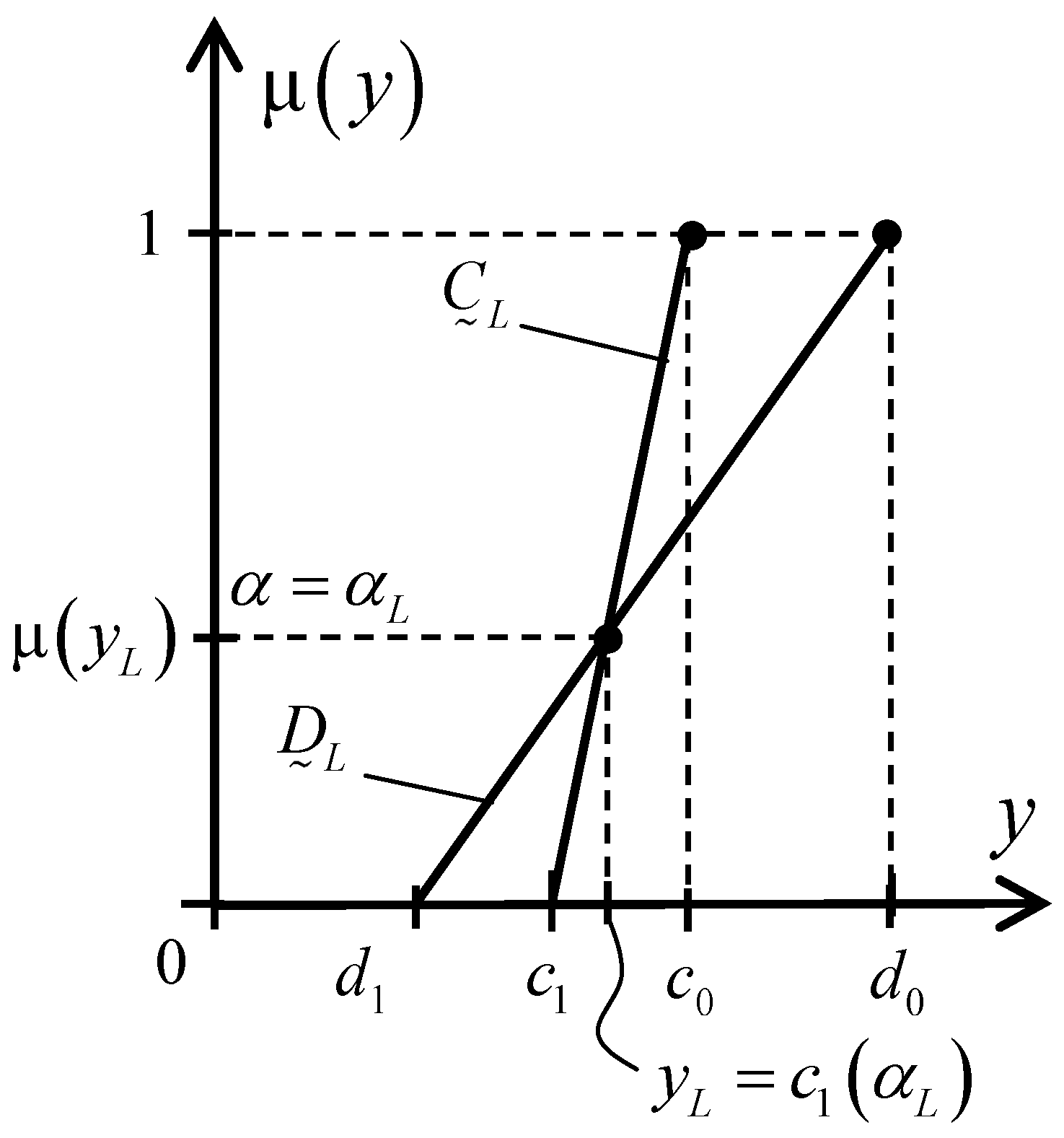
Let us consider the intersection between left branches ${\underset{˜}{C}}_L\cap {\underset{˜}{D}}_L$ and right branches ${\underset{˜}{C}}_R\cap {\underset{˜}{D}}_R$ of the TrFNs $\underset{˜}{C}\in R,\underset{˜}{D}\in R$, separately. The intersection points for left and right branches are the switching points for the resulting analytic models of TrFNs-maximum.

Let us find the solutions (arguments $y_L,y_R$) of the equation:

$${\mu }_{\underset{˜}{C}}\left(y\right)={\mu }_{\underset{˜}{D}}\left(y\right)$$

(9)

by analyzing the intersection of the (a) left branches ${\underset{˜}{C}}_L\cap {\underset{˜}{D}}_L$ of the TrFNs $\underset{˜}{C}\in R,\underset{˜}{D}\in R$ (Figure 2)

$$F_{C_L}\left(y,c_1,c_0\right)\cap F_{D_L}\left(y,d_1,d_0\right):\underset{˜}{C}\in R,\underset{˜}{D}\in R$$

(10)

and (b) right branches ${\underset{˜}{C}}_R\cap {\underset{˜}{D}}_R$ of TrFNs $\underset{˜}{C}\in R,\underset{˜}{D}\in R$ (Figure 3).

$$F_{C_R}\left(y,c_0,c_2\right)\cap F_{D_R}\left(y,d_0,d_2\right):\underset{˜}{C}\in R,\underset{˜}{D}\in R$$

(11)

Let us consider the intersection, for example, of the right branches (Figure 3) in more details.

For intersection (11) between right branches with condition $\alpha \in \left[0,1\right]$ we can form such an equation:

$$c_2\left(\alpha \right)=d_2\left(\alpha \right)=s_2\left(\alpha \right)$$

(12)

which can be rewritten in another style:

$$c_2-\alpha \left(c_2-c_0\right)=d_2-\alpha \left(d_2-d_0\right)$$

(13)

Based on the right components of the horizontal models $C_{\alpha }$ (2) and $D_{\alpha }$ (3):

$$c_2\left(\alpha \right)=c_2-\alpha \left(c_2-c_0\right)$$

(14)

and

$$d_2\left(\alpha \right)=d_2-\alpha \left(d_2-d_0\right).$$

(15)

It is possible to find a vertical coordinate $\alpha ={\alpha }_R$ of the intersection point using (12) and (13):

$${\alpha }_R=\frac{d_2-c_2}{d_2-d_0-c_2+c_0}$$

(16)

In this case we can write:

$${\alpha }_R={\mu }_{\underset{˜}{C}}\left(y_R\right)={\mu }_{\underset{˜}{D}}\left(y_R\right)={\mu }_{\underset{˜}{S}}\left(y_R\right)$$

(17)

using horizontal coordinate $y_R$ for condition (11).

Thus, two couples:

$$\left\{\left(c_2\left({\alpha }_R\right),{\alpha }_R\right),\left(y_R,{\mu }_{\underset{˜}{C}}\left(y_R\right)\right)\right\}$$

(18)

of the intersection point’s coordinates for the (11) can be formed for the right components of the horizontal $\left(c_2\left({\alpha }_R\right),{\alpha }_R\right)$ and vertical $\left(y_R,{\mu }_{\underset{˜}{C}}\left(y_R\right)\right)$ models. In this case: $y_R=c_2\left({\alpha }_R\right),{\mu }_{\underset{˜}{C}}\left(y_R\right)={\alpha }_R$.

It is possible to find the parameter $c_2\left({\alpha }_R\right)$ using (4) and (16):

$$c_2\left({\alpha }_R\right)=c_2-{\alpha }_R\left(c_2-c_0\right)=c_2-\frac{\left(d_2-c_2\right)\left(c_2-c_0\right)}{d_2-d_0-c_2+c_0}$$

(19)

where $c_2\left({\alpha }_R\right)\in \left[\max \left(c_0,d_0\right),\max \left(c_2,d_2\right)\right]$.

For the intersection (10) between the left branches of TrFNs, it is possible to find $\alpha ={\alpha }_L\in \left[0,1\right]$, and using the same approach as for the right branches intersection, we can find two couples:

$$\left\{\left(c_1\left({\alpha }_L\right),{\alpha }_L\right),\left(y_L,{\mu }_{\underset{˜}{C}}\left(y_L\right)\right)\right\}$$

(20)

of the coordinates of intersection point (10), in particular, for left components of the horizontal $\left(c_1\left({\alpha }_L\right),{\alpha }_L\right)$ and vertical $\left(y_L,{\mu }_{\underset{˜}{C}}\left(y_L\right)\right)$ models.

In this case for $y_L=c_1\left({\alpha }_L\right)$ and ${\mu }_{\underset{˜}{C}}\left(y_L\right)={\alpha }_L$ we can find the corresponding parameters ${\alpha }_L$ and $c_1\left({\alpha }_L\right)$ as

$${\alpha }_L=\frac{d_1-c_1}{c_0-c_1-d_0+d_1}$$

(21)

$$c_1\left({\alpha }_L\right)=c_1+{\alpha }_L\left(c_0-c_1\right)=c_1+\frac{\left(d_1-c_1\right)\left(c_0-c_1\right)}{c_0-c_1-d_0+d_1}$$

(22)

where $c_1\left({\alpha }_L\right)\in \left[\max \left(c_1,d_1\right),\max \left(c_0,d_0\right)\right]$.

Finally, we can calculate the values of the coordinates $\left(c_1\left({\alpha }_L\right),{\alpha }_L\right)$ and $\left(c_2\left({\alpha }_R\right),{\alpha }_R\right)$ for the intersection points (10) and (11) using developed analytic models (17), (19), (21), (22), and corresponding data $\left(c_1,d_1,c_0,d_0,c_2,d_2\right)$ for the considered TrFNs $\underset{˜}{C}=\left(c_1,c_0,c_2\right)$ and $\underset{˜}{D}=\left(d_1,d_0,d_2\right)$. The developed models (17), (19), (21), and (22) are universal for any pairs of the TrFNs.

For example, for such relations between TrFNs parameters as $c_1<d_1,c_0>d_0,c_2<d_2$, we can form the horizontal $S_{\alpha }=C_{\alpha }(\vee )D_{\alpha }$ and vertical ${\mu }_{\underset{˜}{S}}\left(y\right)$ models of resulting MF using developed analytic models (17), (19), (21), and (22).

$$\begin{array}{c}{S}_{\alpha }=C_{\alpha }(\vee )D_{\alpha }=\left[c_1\left(\alpha \right)\vee d_1\left(\alpha \right),c_2\left(\alpha \right)\vee d_2\left(\alpha \right)\right]=\\ \left[s_1\left(\alpha \right),s_2\left(\alpha \right)\right]=\\ \left[\left\{\begin{array}{l}{d}_1\left(\alpha \right),\forall \alpha |\alpha \in \left[0,{\alpha }_L\right]\\ c_1\left(\alpha \right),\forall \alpha |\alpha \in \left[{\alpha }_L,1\right]\end{array}\right\},\left\{\begin{array}{l}{c}_2\left(\alpha \right),\forall \alpha |\alpha \in \left[{\alpha }_R,1\right]\\ d_2\left(\alpha \right),\forall \alpha |\alpha \in \left[0,{\alpha }_R\right]\end{array}\right\}\right]\end{array},$$

(23)

$${\mu }_{\underset{˜}{S}}\left(y\right)=\{\begin{array}{l}0,\forall \left(y\le d_1\right)\cup \left(y\ge d_2\right)\\ F_{D_L}\left(y,d_1,d_0\right),\forall \left(d_1<y\le d_1\left({\alpha }_L\right)\right)\\ F_{C_L}\left(y,c_1,c_0\right),\forall \left(c_1\left({\alpha }_L\right)<y\le c_0\right)\\ F_{C_R}\left(y,c_0,c_2\right),\forall \left(c_0<y<c_2\left({\alpha }_R\right)\right)\\ F_{D_R}\left(y,d_0,d_2\right),\forall \left(c_2\left({\alpha }_R\right)<y<d_2\right)\end{array},$$

(24)

where $s_1\left(0\right)=d_1;s_2\left(0\right)=d_2;s_1\left(1\right)=s_2\left(1\right)=c_0;$

$$s_1(\alpha )=\left\{\begin{array}{l}{d}_1+\alpha \left(d_0-d_1\right),\forall \alpha |\alpha \in \left[0,{\alpha }_L\right]\\ c_1+\alpha \left(c_0-c_1\right),\forall \alpha |\alpha \in \left[{\alpha }_L,1\right]\end{array}\right\};$$

$$s_2(\alpha )=\left\{\begin{array}{l}{c}_2-\alpha \left(c_2-c_0\right),\forall \alpha |\alpha \in \left[{\alpha }_R,1\right]\\ d_2-\alpha \left(d_2-d_0\right),\forall \alpha |\alpha \in \left[0,{\alpha }_R\right]\end{array}\right\}.$$

In the Section 3, authors proposed an approach for determining intersection parameters between left (21), (22) and right (16), (19) branches of the initial fuzzy sets $\underset{˜}{C}\in R,\underset{˜}{D}\in R$ that will be used and extended in the following section for creating a set of the resulting analytic models $S_{\alpha }$ and ${\mu }_{\underset{˜}{S}}\left(y\right)$ that can be combined to the generalized computational library as its main components.

4. Synthesis of the Computational Library of Horizontal and Vertical Analytic Models for the Results of the FNs-Maximum Operation

The horizontal $S_{\alpha }$ (23) and the vertical ${\mu }_{\underset{˜}{S}}\left(y\right)$ (24) analytic models for the resulting fuzzy set $\underset{˜}{S}=\underset{˜}{C}(\vee )\underset{˜}{D}$ were synthesized for FNs-maximum operation taking into account the following relations between the TrFNs parameters:

$$c_1<d_1,c_0>d_0,c_2<d_2.$$

(25)

Thus, the analytic models (23) and (24) are validated only for relations (25) in the case of TrFNs $\underset{˜}{C}=\left(c_1,c_0,c_2\right)$ and $\underset{˜}{D}=\left(d_1,d_0,d_2\right)$.

At the same time, TrFNs with different relations $\mathbb{R}$ between their parameters can present a lot of input signals in the real systems and processes [42]:

$$\left\{c_1\mathbb{R}{d}_1,c_0\mathbb{R}{d}_0,c_2\mathbb{R}{d}_2\right\}$$

(26)

where $\mathbb{R}\in \left\{(<),(>)\right\}$.

For each different combination (25) between parameters $\left(c_1,d_1;c_0,d_0;c_2,d_2\right)$ of TrFNs $\left(\underset{˜}{C},\underset{˜}{D}\right)$ it is necessary to synthesize separate horizontal and vertical analytic models of the resulting MF in the case of implementation of the FNs-maximum arithmetic operation.

Let us synthesize the computational library of the resulting fuzzy sets $\underset{˜}{S}$ as corresponding sets of horizontal and vertical analytic models for realization of the FNs-maximum arithmetic operation with TrFNs $\underset{˜}{C}$ and $\underset{˜}{D}$ for different combinations (26) with relations $\mathbb{R}$.

Let us introduce the mask:

$$Mask\left(\underset{˜}{C},\underset{˜}{D}\right)=\left\{m_1,m_2,m_3\right\},$$

(27)

which can be used for recognition of the corresponding relations $\mathbb{R}$ as relations between parameters of the TrFNs $\underset{˜}{C}$ and $\underset{˜}{D}$ [37,42].

The binary indicators $m_1,m_2$, and $m_3$ in the mask (27) can be presented as:

$$\begin{array}{l}{m}_1=\{\begin{array}{l}0, if c_1>d_1\\ 1, if c_1<d_1\end{array};\\ m_2=\{\begin{array}{l}0 ,if c_0>d_0\\ 1 ,if c_0<d_0\end{array};\\ m_3=\{\begin{array}{l}0 ,if c_2>d_2\\ 1 ,if c_2<d_2\end{array}.\end{array}$$

(28)

Using Mask (27) it is possible to form the computational library of the horizontal (29)–(44) and vertical (45)–(52) analytic models $\left\{S{M}_1\dots S{M}_8\right\}$ for the resulting fuzzy sets in the case of execution of FNs-maximum operation with different $\mathbb{R}$ relations (26) between parameters of the TrFNs $\left(\underset{˜}{C},\underset{˜}{D}\right)$, where $S{M}_i,\left(i=1\dots 8\right)$ is the i-th analytic model. The masks (27) and the corresponding models, $S{M}_i,i=1\dots 8$, as components of the computational library $\left\{S{M}_1,S{M}_2,\dots ,S{M}_8\right\}$, are represented in the

Table 1. Models $S{M}_i,\left(i=1\dots 8\right)$ and masks $\left\{m_1,m_2,m_3\right\}$ for different combinations of TrFNs $\underset{˜}{C},\underset{˜}{D}\in R$.

$\mathit{S}{\mathit{M}}_{\mathit{i}},\mathit{i}=1\dots 8$	$\mathit{S}{\mathit{M}}_{\mathbf{1}}$	$\mathit{S}{\mathit{M}}_{\mathbf{2}}$	$\mathit{S}{\mathit{M}}_{\mathbf{3}}$	$\mathit{S}{\mathit{M}}_{\mathbf{4}}$	$\mathit{S}{\mathit{M}}_{\mathbf{5}}$	$\mathit{S}{\mathit{M}}_{\mathbf{6}}$	$\mathit{S}{\mathit{M}}_{\mathbf{7}}$	$\mathit{S}{\mathit{M}}_{\mathbf{8}}$
$\left\{m_1,m_2,m_3\right\}$	$\left\{1,1,1\right\}$	$\left\{1,1,0\right\}$	$\left\{1,0,1\right\}$	$\left\{1,0,0\right\}$	$\left\{0,1,1\right\}$	$\left\{0,1,0\right\}$	$\left\{0,0,1\right\}$	$\left\{0,0,0\right\}$

.

Let us form the computational library of the horizontal $S_{\alpha }=\left[s_1\left(\alpha \right),s_2\left(\alpha \right)\right]$ and the vertical ${\mu }_{\underset{˜}{S}}\left(y\right)$ analytic models of the resulting fuzzy set $\underset{˜}{S}=\underset{˜}{C}(\vee )\underset{˜}{D}$ for different masks (27) according to the Table 1.

The horizontal models $S_{\alpha }$ are synthesized based on the: (a) parameters of $\alpha$-cuts $\left\{c_1\left(\alpha \right),c_2\left(\alpha \right),d_1\left(\alpha \right),d_2\left(\alpha \right)\right\}$, (b) value $\alpha$, and (c) TrFNs’ parameters $\left\{c_1,c_0,c_2,d_1,d_0,d_2\right\}$.

The main components (29)–(44) of the computational library $\left\{S{M}_1,S{M}_2,\dots ,S{M}_8\right\}$ of horizontal analytic models $S_{\alpha }=\left[s_1\left(\alpha \right),s_2\left(\alpha \right)\right]$ are:

-

for $Mask\left(\underset{˜}{C},\underset{˜}{D}\right)=\left\{m_1,m_2,m_3\right\}=\left\{1,1,1\right\}$, model $S{M}_1$:

$$S_{\alpha }=\left[s_1\left(\alpha \right),s_2\left(\alpha \right)\right]=\left[\left\{d_1\left(\alpha \right),\forall \alpha |\alpha \in \left[0,1\right]\right\},\left\{d_2\left(\alpha \right),\forall \alpha |\alpha \in \left[0,1\right]\right\}\right],$$

(29)

$$\left[s_1\left(\alpha \right),s_2\left(\alpha \right)\right]=\left[\left\{d_1+\alpha \left(d_0-d_1\right),\forall \alpha |\alpha \in \left[0,1\right]\right\},\left\{d_2-\alpha \left(d_2-d_0\right),\forall \alpha |\alpha \in \left[0,1\right]\right\}\right];$$

(30)

-

for $Mask\left(\underset{˜}{C},\underset{˜}{D}\right)=\left\{m_1,m_2,m_3\right\}=\left\{1,1,0\right\}$, model $S{M}_2$:

$$S_{\alpha }=\left[s_1\left(\alpha \right),s_2\left(\alpha \right)\right]=\left[\left\{d_1\left(\alpha \right),\forall \alpha |\alpha \in \left[0,1\right]\right\},\left\{\begin{array}{l}{d}_2\left(\alpha \right),\forall \alpha |\alpha \in \left[{\alpha }_R,1\right]\\ c_2\left(\alpha \right),\forall \alpha |\alpha \in \left[0,{\alpha }_R\right]\end{array}\right\}\right],$$

(31)

$$\left[s_1\left(\alpha \right),s_2\left(\alpha \right)\right]=\left[\left\{d_1+\alpha \left(d_0-d_1\right),\forall \alpha |\alpha \in \left[0,1\right]\right\},\left\{\begin{array}{l}{d}_2-\alpha \left(d_2-d_0\right),\forall \alpha |\alpha \in \left[{\alpha }_R,1\right]\\ c_2-\alpha \left(c_2-c_0\right),\forall \alpha |\alpha \in \left[0,{\alpha }_R\right]\end{array}\right\}\right];$$

(32)

-

for $Mask\left(\underset{˜}{C},\underset{˜}{D}\right)=\left\{m_1,m_2,m_3\right\}=\left\{1,0,1\right\}$, model $S{M}_3$:

$$S_{\alpha }=\left[s_1\left(\alpha \right),s_2\left(\alpha \right)\right]=\left[\left\{\begin{array}{l}{d}_1\left(\alpha \right),\forall \alpha |\alpha \in \left[0,{\alpha }_L\right]\\ c_1\left(\alpha \right),\forall \alpha |\alpha \in \left[{\alpha }_L,1\right]\end{array}\right\},\left\{\begin{array}{l}{c}_2\left(\alpha \right),\forall \alpha |\alpha \in \left[{\alpha }_R,1\right]\\ d_2\left(\alpha \right),\forall \alpha |\alpha \in \left[0,{\alpha }_R\right]\end{array}\right\}\right],$$

(33)

$$\left[s_1\left(\alpha \right),s_2\left(\alpha \right)\right]=\left[\left\{\begin{array}{l}{d}_1+\alpha \left(d_0-d_1\right),\forall \alpha |\alpha \in \left[0,{\alpha }_L\right]\\ c_1+\alpha \left(c_0-c_1\right),\forall \alpha |\alpha \in \left[{\alpha }_L,1\right]\end{array}\right\},\left\{\begin{array}{l}{c}_2-\alpha \left(c_2-c_0\right),\forall \alpha |\alpha \in \left[{\alpha }_R,1\right]\\ d_2-\alpha \left(d_2-d_0\right),\forall \alpha |\alpha \in \left[0,{\alpha }_R\right]\end{array}\right\}\right];$$

(34)

-

for $Mask\left(\underset{˜}{C},\underset{˜}{D}\right)=\left\{m_1,m_2,m_3\right\}=\left\{1,0,0\right\}$, model $S{M}_4$:

$$S_{\alpha }=\left[s_1\left(\alpha \right),s_2\left(\alpha \right)\right]=\left[\left\{\begin{array}{l}{d}_1\left(\alpha \right),\forall \alpha |\alpha \in \left[0,{\alpha }_L\right]\\ c_1\left(\alpha \right),\forall \alpha |\alpha \in \left[{\alpha }_L,1\right]\end{array}\right\},\left\{c_2\left(\alpha \right),\forall \alpha |\alpha \in \left[0,1\right]\right\}\right]$$

(35)

$$\left[s_1\left(\alpha \right),s_2\left(\alpha \right)\right]=\left[\left\{\begin{array}{l}{d}_1+\alpha \left(d_0-d_1\right),\forall \alpha |\alpha \in \left[0,{\alpha }_L\right]\\ c_1+\alpha \left(c_0-c_1\right),\forall \alpha |\alpha \in \left[{\alpha }_L,1\right]\end{array}\right\},\left\{c_2-\alpha \left(c_2-c_0\right),\forall \alpha |\alpha \in \left[0,1\right]\right\}\right];$$

(36)

-

for $Mask\left(\underset{˜}{C},\underset{˜}{D}\right)=\left\{m_1,m_2,m_3\right\}=\left\{0,1,1\right\}$, model $S{M}_5$:

$$S_{\alpha }=\left[s_1\left(\alpha \right),s_2\left(\alpha \right)\right]=\left[\left\{\begin{array}{l}{c}_1\left(\alpha \right),\forall \alpha |\alpha \in \left[0,{\alpha }_L\right]\\ d_1\left(\alpha \right),\forall \alpha |\alpha \in \left[{\alpha }_L,1\right]\end{array}\right\},\left\{d_2\left(\alpha \right),\forall \alpha |\alpha \in \left[0,1\right]\right\}\right],$$

(37)

$$\left[s_1\left(\alpha \right),s_2\left(\alpha \right)\right]=\left[\left\{\begin{array}{l}{c}_1+\alpha \left(c_0-c_1\right),\forall \alpha |\alpha \in \left[0,{\alpha }_L\right]\\ d_1+\alpha \left(d_0-d_1\right),\forall \alpha |\alpha \in \left[{\alpha }_L,1\right]\end{array}\right\},\left\{d_2-\alpha \left(d_2-d_0\right),\forall \alpha |\alpha \in \left[0,1\right]\right\}\right];$$

(38)

-

for $Mask\left(\underset{˜}{C},\underset{˜}{D}\right)=\left\{m_1,m_2,m_3\right\}=\left\{0,1,0\right\}$, model $S{M}_6$:

$$S_{\alpha }=\left[s_1\left(\alpha \right),s_2\left(\alpha \right)\right]=\left[\left\{\begin{array}{l}{c}_1\left(\alpha \right),\forall \alpha |\alpha \in \left[0,{\alpha }_L\right]\\ d_1\left(\alpha \right),\forall \alpha |\alpha \in \left[{\alpha }_L,1\right]\end{array}\right\},\left\{\begin{array}{l}{d}_2\left(\alpha \right),\forall \alpha |\alpha \in \left[{\alpha }_R,1\right]\\ c_2\left(\alpha \right),\forall \alpha |\alpha \in \left[0,{\alpha }_R\right]\end{array}\right\}\right],$$

(39)

$$\left[s_1\left(\alpha \right),s_2\left(\alpha \right)\right]=\left[\left\{\begin{array}{l}{c}_1+\alpha \left(c_0-c_1\right),\forall \alpha |\alpha \in \left[0,{\alpha }_L\right]\\ d_1+\alpha \left(d_0-d_1\right),\forall \alpha |\alpha \in \left[{\alpha }_L,1\right]\end{array}\right\},\left\{\begin{array}{l}{d}_2-\alpha \left(d_2-d_0\right),\forall \alpha |\alpha \in \left[{\alpha }_R,1\right]\\ c_2-\alpha \left(c_2-c_0\right),\forall \alpha |\alpha \in \left[0,{\alpha }_R\right]\end{array}\right\}\right];$$

(40)

-

for $Mask\left(\underset{˜}{C},\underset{˜}{D}\right)=\left\{m_1,m_2,m_3\right\}=\left\{0,0,1\right\}$, model $S{M}_7$:

$$S_{\alpha }=\left[s_1\left(\alpha \right),s_2\left(\alpha \right)\right]=\left[\left\{c_1\left(\alpha \right),\forall \alpha |\alpha \in \left[0,1\right]\right\},\left\{\begin{array}{l}{c}_2\left(\alpha \right),\forall \alpha |\alpha \in \left[{\alpha }_R,1\right]\\ d_2\left(\alpha \right),\forall \alpha |\alpha \in \left[0,{\alpha }_R\right]\end{array}\right\}\right],$$

(41)

$$\left[s_1\left(\alpha \right),s_2\left(\alpha \right)\right]=\left[\left\{c_1+\alpha \left(c_0-c_1\right),\forall \alpha |\alpha \in \left[0,1\right]\right\},\left\{\begin{array}{l}{c}_2-\alpha \left(c_2-c_0\right),\forall \alpha |\alpha \in \left[{\alpha }_R,1\right]\\ d_2-\alpha \left(d_2-d_0\right),\forall \alpha |\alpha \in \left[0,{\alpha }_R\right]\end{array}\right\}\right];$$

(42)

-

for $Mask\left(\underset{˜}{C},\underset{˜}{D}\right)=\left\{m_1,m_2,m_3\right\}=\left\{0,0,0\right\}$, model $S{M}_8$:

$$S_{\alpha }=\left[s_1\left(\alpha \right),s_2\left(\alpha \right)\right]=\left[\left\{c_1\left(\alpha \right),\forall \alpha |\alpha \in \left[0,1\right]\right\},\left\{c_2\left(\alpha \right),\forall \alpha |\alpha \in \left[0,1\right]\right\}\right],$$

(43)

$$\left[s_1\left(\alpha \right),s_2\left(\alpha \right)\right]=\left[\left\{c_1+\alpha \left(c_0-c_1\right),\forall \alpha |\alpha \in \left[0,1\right]\right\},\left\{c_2-\alpha \left(c_2-c_0\right),\forall \alpha |\alpha \in \left[0,1\right]\right\}\right].$$

(44)

The vertical (45)–(52) models ${\mu }_{\underset{˜}{S}}\left(y\right)$ of the resulting fuzzy sets $\underset{˜}{S}=\underset{˜}{C}(\vee )\underset{˜}{D}$ are synthesized based on the: (a) left and right functions $\left\{F_{C_L},F_{C_R},F_{D_L},F_{D_R}\right\}$, and (b) TrFNs’ parameters $\left\{c_1,c_0,c_2,d_1,d_0,d_2\right\}$.

The main components (45)–(52) of the computational library $\left\{S{M}_1,S{M}_2,\dots ,S{M}_8\right\}$ of the vertical analytic models ${\mu }_{\underset{˜}{S}}\left(y\right)$ are:

-

for the $Mask\left(\underset{˜}{C},\underset{˜}{D}\right)=\left\{m_1,m_2,m_3\right\}=\left\{1,1,1\right\}$, model $S{M}_1$:

$${\mu }_{\underset{˜}{S}}\left(y\right)=\{\begin{array}{l}0,\forall \left(y\le d_1\right)\cup \left(y\ge d_2\right)\\ F_{D_L}\left(y,d_1,d_0\right),\forall \left(d_1<y\le d_0\right)\\ F_{D_R}\left(y,d_0,d_2\right),\forall \left(d_0<y<d_2\right)\end{array}=\{\begin{array}{l}0,\forall \left(y\le d_1\right)\cup \left(y\ge d_2\right)\\ \left(y-d_1\right)/\left(d_0-d_1\right),\forall \left(d_1<y\le d_0\right)\\ \left(d_2-y\right)/\left(d_2-d_0\right),\forall \left(d_0<y<d_2\right)\end{array};$$

(45)

-

for the $Mask\left(\underset{˜}{C},\underset{˜}{D}\right)=\left\{m_1,m_2,m_3\right\}=\left\{1,1,0\right\}$, model $S{M}_2$:

$${\mu }_{\underset{˜}{S}}\left(y\right)=\{\begin{array}{l}0,\forall \left(y\le d_1\right)\cup \left(y\ge c_2\right)\\ F_{D_L}\left(y,d_1,d_0\right),\forall \left(d_1<y\le d_0\right)\\ F_{D_R}\left(y,d_0,d_2\right),\forall \left(d_0<y<c_2\left({\alpha }_R\right)\right)\\ F_{C_R}\left(y,c_0,c_2\right),\forall \left(c_2\left({\alpha }_R\right)\le y<c_2\right)\end{array}=\{\begin{array}{l}0,\forall \left(y\le d_1\right)\cup \left(y\ge c_2\right)\\ \left(y-d_1\right)/\left(d_0-d_1\right),\forall \left(d_1<y\le d_0\right)\\ \left(d_2-y\right)/\left(d_2-d_0\right),\forall \left(d_0<y<c_2\left({\alpha }_R\right)\right)\\ \left(c_2-y\right)/\left(c_2-c_0\right),\forall \left(c_2\left({\alpha }_R\right)\le y<c_2\right)\end{array};$$

(46)

-

for the $Mask\left(\underset{˜}{C},\underset{˜}{D}\right)=\left\{m_1,m_2,m_3\right\}=\left\{1,0,1\right\}$, model $S{M}_3$:

$${\mu }_{\underset{˜}{S}}\left(y\right)=\{\begin{array}{l}0,\forall \left(y\le d_1\right)\cup \left(y\ge d_2\right)\\ F_{D_L}\left(y,d_1,d_0\right),\forall \left(d_1<y\le c_1\left({\alpha }_L\right)\right)\\ F_{C_L}\left(y,c_1,c_0\right),\forall (c_1\left({\alpha }_L\right)<y\le c_0)\\ F_{C_R}\left(y,c_0,c_2\right),\forall \left(c_0<y<c_2\left({\alpha }_R\right)\right)\\ F_{D_R}\left(y,d_0,d_2\right),\forall (c_2\left({\alpha }_R\right)\le y<d_2)\end{array}=\{\begin{array}{l}0,\forall \left(y\le d_1\right)\cup \left(y\ge d_2\right)\\ \left(y-d_1\right)/\left(d_0-d_1\right),\forall \left(d_1<y\le c_1\left({\alpha }_L\right)\right)\\ \left(y-c_1\right)/\left(c_0-c_1\right),\forall \left(c_1\left({\alpha }_L\right)<y\le c_0\right)\\ \left(c_2-y\right)/\left(c_2-c_0\right),\forall \left(c_0<y<c_2\left({\alpha }_R\right)\right)\\ \left(d_2-y\right)/\left(d_2-d_0\right),\forall \left(c_2\left({\alpha }_R\right)\le y<d_2\right)\end{array};$$

(47)

-

for the $Mask\left(\underset{˜}{C},\underset{˜}{D}\right)=\left\{m_1,m_2,m_3\right\}=\left\{1,0,0\right\}$, model $S{M}_4$:

$${\mu }_{\underset{˜}{S}}\left(y\right)=\{\begin{array}{l}0,\forall \left(y\le d_1\right)\cup \left(y\ge c_2\right)\\ F_{D_L}\left(y,d_1,d_0\right),\forall \left(d_1<y\le c_1\left({\alpha }_L\right)\right)\\ F_{C_L}\left(y,c_1,c_0\right),\forall \left(c_1\left({\alpha }_L\right)<y\le c_0\right)\\ F_{C_R}\left(y,c_0,c_2\right),\forall \left(c_0<y<c_2\right)\end{array}=\{\begin{array}{l}0,\forall \left(y\le d_1\right)\cup \left(y\ge c_2\right)\\ \left(y-d_1\right)/\left(d_0-d_1\right),\forall \left(d_1<y\le c_1\left({\alpha }_L\right)\right)\\ \left(y-c_1\right)/\left(c_0-c_1\right),\forall \left(c_1\left({\alpha }_L\right)<y\le c_0\right)\\ \left(c_2-y\right)/\left(c_2-c_0\right),\forall \left(c_0<y<c_2\right)\end{array};$$

(48)

-

for the $Mask\left(\underset{˜}{C},\underset{˜}{D}\right)=\left\{m_1,m_2,m_3\right\}=\left\{0,1,1\right\}$, model $S{M}_5$:

$${\mu }_{\underset{˜}{S}}\left(y\right)=\{\begin{array}{l}0,\forall \left(y\le c_1\right)\cup \left(y\ge d_2\right)\\ F_{C_L}\left(y,c_1,c_0\right),\forall \left(c_1<y\le c_1\left({\alpha }_L\right)\right)\\ F_{D_L}\left(y,d_1,d_0\right),\forall \left(c_1\left({\alpha }_L\right)<y\le d_0\right)\\ F_{D_R}\left(y,d_0,d_2\right),\forall \left(d_0<y<d_2\right)\end{array}=\{\begin{array}{l}0,\forall \left(y\le c_1\right)\cup \left(y\ge d_2\right)\\ \left(y-c_1\right)/\left(c_0-c_1\right),\forall \left(c_1<y\le c_1\left({\alpha }_L\right)\right)\\ \left(y-d_1\right)/\left(d_0-d_1\right),\forall \left(c_1\left({\alpha }_L\right)<y\le d_0\right)\\ \left(d_2-y\right)/\left(d_2-d_0\right),\forall \left(d_0<y<d_2\right)\end{array};$$

(49)

-

for the $Mask\left(\underset{˜}{C},\underset{˜}{D}\right)=\left\{m_1,m_2,m_3\right\}=\left\{0,1,0\right\}$, model $S{M}_6$:

$${\mu }_{\underset{˜}{S}}\left(y\right)=\{\begin{array}{l}0,\forall \left(y\le c_1\right)\cup \left(y\ge c_2\right)\\ F_{C_L}\left(y,c_1,c_0\right),\forall \left(c_1<y\le c_1\left({\alpha }_L\right)\right)\\ F_{D_L}\left(y,d_1,d_0\right),\forall (c_1\left({\alpha }_L\right)<y\le d_0)\\ F_{D_R}\left(y,d_0,d_2\right),\forall \left(d_0<y<c_2\left({\alpha }_R\right)\right)\\ F_{C_R}\left(y,c_0,c_2\right),\forall (c_2\left({\alpha }_R\right)\le y<c_2)\end{array}=\{\begin{array}{l}0,\forall \left(y\le c_1\right)\cup \left(y\ge c_2\right)\\ \left(y-c_1\right)/\left(c_0-c_1\right),\forall \left(c_1<y\le c_1\left({\alpha }_L\right)\right)\\ \left(y-d_1\right)/\left(d_0-d_1\right),\forall \left(c_1\left({\alpha }_L\right)<y\le d_0\right)\\ \left(d_2-y\right)/\left(d_2-c_0\right),\forall \left(d_0<y<c_2\left({\alpha }_R\right)\right)\\ \left(c_2-y\right)/\left(c_2-c_0\right),\forall \left(c_2\left({\alpha }_R\right)\le y<c_2\right)\end{array};$$

(50)

-

for the $Mask\left(\underset{˜}{C},\underset{˜}{D}\right)=\left\{m_1,m_2,m_3\right\}=\left\{0,0,1\right\}$, model $S{M}_7$:

$${\mu }_{\underset{˜}{S}}\left(y\right)=\{\begin{array}{l}0,\forall \left(y\le c_1\right)\cup \left(y\ge d_2\right)\\ F_{C_L}\left(y,c_1,c_0\right),\forall \left(c_1<y\le c_0\right)\\ F_{C_R}\left(y,c_0,c_2\right),\forall \left(c_0<y<c_2\left({\alpha }_R\right)\right)\\ F_{D_R}\left(y,d_0,d_2\right),\forall \left(c_2\left({\alpha }_R\right)\le y<d_2\right)\end{array}=\{\begin{array}{l}0,\forall \left(y\le c_1\right)\cup \left(y\ge d_2\right)\\ \left(y-c_1\right)/\left(c_0-c_1\right),\forall \left(c_1<y\le c_0\right)\\ \left(c_2-y\right)/\left(c_2-c_0\right),\forall \left(c_0<y<c_2\left({\alpha }_R\right)\right)\\ \left(d_2-y\right)/\left(d_2-d_0\right),\forall \left(c_2\left({\alpha }_R\right)\le y<d_2\right)\end{array}$$

(51)

-

for the $Mask\left(\underset{˜}{C},\underset{˜}{D}\right)=\left\{m_1,m_2,m_3\right\}=\left\{0,0,0\right\}$, model $S{M}_8$:

$${\mu }_{\underset{˜}{S}}\left(y\right)=\{\begin{array}{l}0,\forall \left(y\le c_1\right)\cup \left(y\ge c_2\right)\\ F_{C_L}\left(y,c_1,c_0\right),\forall \left(c_1<y\le c_0\right)\\ F_{C_R}\left(y,c_0,c_2\right),\forall \left(c_0<y<c_2\right)\end{array}=\{\begin{array}{l}0,\forall \left(y\le c_1\right)\cup \left(y\ge c_2\right)\\ \left(y-c_1\right)/\left(c_0-c_1\right),\forall \left(c_1<y\le c_0\right)\\ \left(c_2-y\right)/\left(c_2-c_0\right),\forall \left(c_0<y<c_2\right)\end{array}.$$

(52)

Thus, formation of the mask (27) for any pair $\left(\underset{˜}{C},\underset{˜}{D}\right)$ of the fuzzy numbers with various relations (26) between their parameters $\left\{c_1,c_0,c_2,d_1,d_0,d_2\right\}$ allows: (a) to determine (automatically) the corresponding horizontal and vertical analytic models of the resulting fuzzy set based on the developed computational library (29)–(52), and (b) to use these analytic models for the one-step computation of the resulting membership function values ${\mu }_{\underset{˜}{S}}\left(y\right)$ for different values of the variable $y$. In Section 5, the authors provide a numerical example of the fuzzy data processing based on the application of the computational library (29)–(52).

5. Example: Computational Library Application

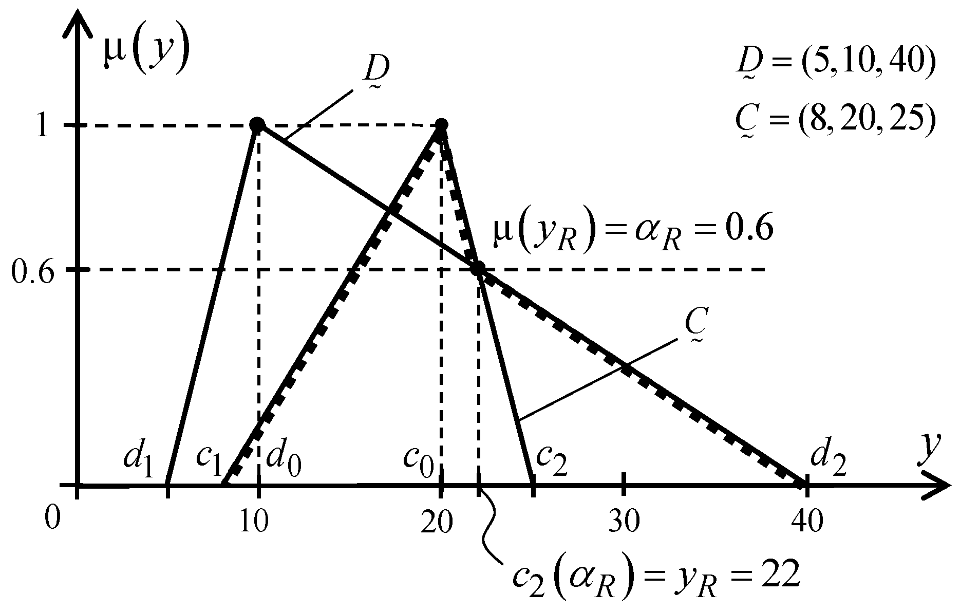
Let us consider an example with the realization of the FNs-maximum operation for the TrFNs (Figure 4):

$$\underset{˜}{C}=\left(8,20,25\right),\underset{˜}{D}=\left(5,10,40\right)$$

(53)

where parameters of the TrFNs are: $c_1=8;d_1=5;c_0=20;d_0=10;c_2=25;d_2=40$.

In this case, the relations (21) can be defined as

$$c_1>d_1;c_0>d_0;c_2<d_2.$$

(54)

Using (27), (28), and (54) we can automatically determine:

(a)

the corresponding $Mask\left(\underset{˜}{C},\underset{˜}{D}\right)=\left\{m_1,m_2,m_3\right\}=\left\{0,0,1\right\}$,

(b)

and the corresponding model $S{M}_7$ from the computational library of models $\left\{S{M}_1,S{M}_2,\dots ,S{M}_8\right\}$ (Table 1).

Let us calculate the coordinates $\left(c_2\left({\alpha }_R\right),{\alpha }_R\right)$ for the intersection point (11) of the given (53) fuzzy numbers $\left(\underset{˜}{C},\underset{˜}{D}\right)$ according to (19) and (16):

$$c_2\left({\alpha }_R\right)=c_2-\frac{\left(d_2-c_2\right)\left(c_2-c_0\right)}{d_2-d_0-c_2+c_0}=25-\frac{\left(40-25\right)\left(25-20\right)}{40-10-25+20}=22.0,$$

(55)

$${\alpha }_R=\frac{d_2-c_2}{d_2-d_0-c_2+c_0}=\frac{40-25}{40-10-25+20}=0.6.$$

(56)

In the next step, we can choose (for recognized $S{M}_7$) the corresponding horizontal $S_{\alpha }$ (41)–(42) and vertical ${\mu }_{\underset{˜}{S}}\left(y\right)$ (51) models from the computational library (29)–(52) of the resulting analytic models. We further present the resulting horizontal $S_{\alpha }=C_{\alpha }(\vee )D_{\alpha }$ (57) and vertical ${\mu }_{\underset{˜}{S}}\left(y\right)$ (58) models (Figure 4) for FNs-maximum $\underset{˜}{S}=\underset{˜}{C}(\vee )\underset{˜}{D}$:

$$S_{\alpha }=C_{\alpha }(\vee )D_{\alpha }=\left[\begin{array}{l}\left\{c_1+\alpha \left(c_0-c_1\right),\forall \alpha |\alpha \in \left[0,1\right]\right\},\\ \left\{\begin{array}{l}{c}_2-\alpha \left(c_2-c_0\right),\forall \alpha |\alpha \in \left[{\alpha }_R,1\right]\\ d_2-\alpha \left(d_2-d_0\right),\forall \alpha |\alpha \in \left[0,{\alpha }_R\right]\end{array}\right\}\end{array}\right]=\left[\begin{array}{l}\left\{8+12\alpha ,\forall \alpha |\alpha \in \left[0,1\right]\right\},\\ \left\{\begin{array}{l}25-5\alpha ,\forall \alpha |\alpha \in \left[0.6,1\right]\\ 40-30\alpha ,\forall \alpha |\alpha \in \left[0,0.6\right]\end{array}\right\}\end{array}\right],$$

(57)

$${\mu }_{\underset{˜}{S}}\left(y\right)=\{\begin{array}{l}0,\forall \left(y\le c_1\right)\cup \left(y\ge d_2\right)\\ \frac{\left(y-c_1\right)}{\left(c_0-c_1\right)},\forall \left(c_1<y\le c_0\right)\\ \frac{\left(c_2-y\right)}{\left(c_2-c_0\right)},\forall \left(c_0<y<c_2\left({\alpha }_R\right)\right)\\ \frac{\left(d_2-y\right)}{\left(d_2-d_0\right)},\forall \left(c_2\left({\alpha }_R\right)\le y<d_2\right)\end{array}=\{\begin{array}{l}0,\forall \left(y\le 8\right)\cup \left(y\ge 40\right)\\ \frac{\left(y-8\right)}{12},\forall \left(8<y\le 20\right)\\ \frac{\left(25-y\right)}{5},\forall \left(20<y<22\right)\\ \frac{\left(40-y\right)}{30},\forall \left(22\le y<40\right)\end{array}.$$

(58)

The models (57) and (58) are the exact analytic models that help to obtain the exact calculation results.

The horizontal analytic model (57) has a capacity to calculate $S_{\alpha }$ of the resulting fuzzy set $\underset{˜}{S}=\underset{˜}{C}(\vee )\underset{˜}{D}$ for any $\alpha |\alpha \in \left[0,1\right]$. For example, for $\alpha =0.35$ the resulting $S_{\alpha }$ will be calculated as $S_{\alpha }=\left[8+12\alpha ,40-30\alpha \right]=\left[8+12\cdot 0.35,40-30\cdot 0.35\right]=\left[12.2,29.5\right]$.

Using the vertical model (58), it is easy to calculate the value of ${\mu }_{\underset{˜}{S}}\left(y^{\ast }\right)$ of the resulting membership function ${\mu }_{\underset{˜}{S}}\left(y\right)$ for any required value of $y=y^{\ast }$. For example, for $y^{\ast }=21,1$ we have the exact result of ${\mu }_{\underset{˜}{S}}\left(21.1\right)=0.78$, and for $y^{\ast }=23.05$ ${\mu }_{\underset{˜}{S}}\left(23.05\right)=0.565$.

Let us compare these pairs of exact results $\left(y^{\ast }=21.1;{\mu }_{\underset{˜}{S}}\left(21.1\right)=0.78\right)$ and $\left(y^{\ast }=23.05;{\mu }_{\underset{˜}{S}}\left(23.05\right)=0.565\right)$, obtained using the developed computational library of analytic models (45)–(52), with results obtained using the traditional $\alpha$-cut approach [29,30,43], where according to (1) ${\alpha }_i={\alpha }_{i-1}+\delta \alpha ,\left(i=1,2,\dots ,N\right)$.

Let us choose, for example, $N=4$. In this case, $\delta \alpha =0.25$ and the horizontal models $S_{\alpha }$ for the FNs-maximum $\underset{˜}{S}=\underset{˜}{C}(\vee )\underset{˜}{D}$ can be calculated using FNs-maximum algorithm (8), initial data $S_{\alpha =0}=[8,40]$ for $\alpha =0$, and the iterative procedure ${\alpha }_i={\alpha }_{i-1}+0.25,\left(i=1,2,3,4\right),$ as:

$$S_{\alpha =0.25}=[11,32.5];S_{\alpha =0.5}=[14,25];S_{\alpha =0.75}=[17,21.25];\mathrm{and}{S}_{\alpha =1}=[20,20].$$

For determining each component of $S_{\alpha ={\alpha }_i}$ of the corresponding horizontal model it is necessary to realize a multi-step calculation procedure using different formulas:

(a)

calculate $c_1\left({\alpha }_i\right)$, using the horizontal model (4-1) for the left branch of the TrFN $\underset{˜}{C}$;

(b)

calculate $c_2\left({\alpha }_i\right)$, using the horizontal model (4-1) for the right branch of the TrFN $\underset{˜}{C}$;

(c)

calculate $d_1\left({\alpha }_i\right)$, using the horizontal model (6) for the left branch of the TrFN $\underset{˜}{D}$;

(d)

calculate $d_2\left({\alpha }_i\right)$, using the horizontal model (6) for the right branch of the TrFN $\underset{˜}{D}$;

(e)

determine $s_1\left({\alpha }_i\right)$ based on the horizontal model (8) for the left branch of the resulting fuzzy set $\underset{˜}{S}$ and using the Max-operator: $s_1\left({\alpha }_i\right)=c_1\left({\alpha }_i\right)\vee d_1\left({\alpha }_i\right)=\max \left\{c_1\left({\alpha }_i\right),d_1\left({\alpha }_i\right)\right\}$;

(f)

determine $s_2\left({\alpha }_i\right)$ based on the horizontal model (8) for the right branch of the resulting fuzzy set $\underset{˜}{S}$ and using the Max-operator: $s_2\left({\alpha }_i\right)=c_2\left({\alpha }_i\right)\vee d_2\left({\alpha }_i\right)=\max \left\{c_2\left({\alpha }_i\right),d_2\left({\alpha }_i\right)\right\}$.

The corresponding resulting fuzzy set is

$$\underset{˜}{S}={\displaystyle \sum _{i=0}^{2N}\frac{{\mu }_{\underset{˜}{S}}\left(y_i\right)}{y_i}}=\frac{0}{8}+\frac{0.25}{11}+\frac{0.5}{14}+\frac{0.75}{17}+\frac{1}{20}+\frac{0.75}{21.25}+\frac{0.5}{25}+\frac{0.25}{32.5}+\frac{0}{40}$$

(59)

If $y^{\ast }\notin \mathrm{supp}\left(\underset{˜}{S}\right),$ where $\mathrm{supp}\left(\underset{˜}{S}\right)=\left\{y:{\mu }_{\underset{˜}{S}}\left(y\right)>0\right\}=\left\{\left(8\right),11,14,17,20,21.25,25,32.5,\left(40\right)\right\}$ according to (59), then, for example, as the next step, it is necessary to implement the polynomial approximation or linear interpolation procedures. Let us find ${\mu }_{\underset{˜}{S}}\left(y^{\ast }\right)$ for $y_i<y^{\ast }<y_{i+1}$ based on the fuzzy set (59) and the linear interpolation approach:

$${\mu }_{\underset{˜}{S}}\left(y^{\ast }\right)={\mu }_{\underset{˜}{S}}\left(y_i\right)+\frac{{\mu }_{\underset{˜}{S}}\left(y_{i+1}\right)-{\mu }_{\underset{˜}{S}}\left(y_i\right)}{y_{i+1}-y_i}\left(y^{\ast }-y_i\right).$$

(60)

For example, (a) for $y^{\ast }=22$, $y_5<y^{\ast }<y_6$, we can calculate ${\mu }_{\underset{˜}{S}}\left(22\right)$ using (60) as:

$${\mu }_{\underset{˜}{S}}\left(22\right)={\mu }_{\underset{˜}{S}}\left(y_5\right)+\frac{{\mu }_{\underset{˜}{S}}\left(y_6\right)-{\mu }_{\underset{˜}{S}}\left(y_5\right)}{y_6-y_5}\left(22-y_5\right)=0.75+\frac{0.5-0.75}{25-21.25}\left(22-21.25\right)=0.6786;$$

(61)

(b) for $y^{\ast }=21.1$, $y_4<y^{\ast }<y_5$:

$${\mu }_{\underset{˜}{S}}\left(21.1\right)=1+\frac{0.75-1}{21.25-20}\left(21.1-20\right)=0.78;$$

(62)

(c) for $y^{\ast }=23.05$, $y_5<y^{\ast }<y_6$:

$${\mu }_{\underset{˜}{S}}\left(23.05\right)==0.75+\frac{0.5-0.75}{25-21.25}\left(23.05-21.25\right)=0.622.$$

(63)

The authors further present the corresponding interpolation errors comparing with the calculations based on the analytic model (58, obtained from the developed computational library:

$${\Delta }_a=\left|0.6-0.6786\right|=0.0786, \mathrm{for} y^{\ast }=22;$$

$${\Delta }_b=\left|0.78-0.78\right|=0, \mathrm{for} y^{\ast }=21.1;$$

$${\Delta }_c=\left|0.565-0.622\right|=0.057, \mathrm{for} y^{\ast }=23.05,$$

that corresponds (in percentage) to the relative values of 13,10%, 0,00%, and 10.08%.

These examples show that the interpolation errors will exist for the condition $y_5<y^{\ast }<y_6$. In a general case, these errors exist for the values of $y^{\ast }$, which belongs to the intervals $\left[y_k,y_{k+1}\right]$ and $\left[y_j,y_{j+1}\right]$ with corresponding conditions: $c_1\left({\alpha }_L\right)\in \left[y_k,y_{k+1}\right]$ and $c_2\left({\alpha }_R\right)\in \left[y_j,y_{j+1}\right]$. It is possible to decrease the interpolation errors by increasing the number $N$ of $\alpha$-cuts, but in this case, the resulting fuzzy set (59) will have more components and the computing time will be significantly increased due to the multi-step calculations.

The computational library was realized in the computing development environment Visual Studio 2013 using the C# (Windows Forms) programming language. The link to the program code is https://bitbucket.org/ykondratenko/computelib/src. Modeling results confirm that the analytic models (as components of the computational library (45)–(52)) proposed in this article provide efficient one-step calculation of the resulting membership function for values ${\mu }_{\underset{˜}{S}}\left(y^{\ast }\right)$ with higher accuracy and improved calculation speed compared with $\alpha$-cuts approach and Max-Min convolution, which are based on the multi-step calculation procedures.

6. Conclusions

The main contribution of this work deals with the development of the methodological approach and the “one-step” calculation algorithm for fuzzy data processing based on: (a) evaluation of the relations between FNs parameters using a proposed three-components mask; (b) development of the universal horizontal and vertical analytic models for the resulting fuzzy sets, which provides a high accuracy of fuzzy data processing; and (c) creation of the generalized computational library of the resulting analytic models that allows a realization of “one-step” computing for various combinations between the FNs parameters.

The proposed computational library of the horizontal and vertical analytic models (29)–(52) allows more efficient data processing in real-time. When it comes to application and realization of FNs-maximum operations with triangular fuzzy numbers parameters, it was necessary to choose the preliminary synthesized analytic models from the computational library based on the TrFNs parameters. This approach leads to significant increasing computational speed of the data processing since the usage of the proposed library of horizontal and vertical models allows realizing only one-step computing automation mode in fuzzy data processing, in particular, for computing the FNs-maximum arithmetic operation $\underset{˜}{S}=\underset{˜}{C}(\vee )\underset{˜}{D}$.

In some practical applications, it is necessary to represent Big Data (random time-series, random consequences, etc.) as compressed fuzzy sets (fuzzy numbers) using aggregation algorithms for different data streams [29,46,47]. It is possible to use a four-step algorithm for “Big Data-fuzzy data” processing of such random streams or consequences using the proposed computational library:

(a)

Each random stream or consequence of Big Data can be transformed into the compressed fuzzy set (fuzzy number) [1,29,40]. Examples of such random sequences’ transformations are presented in References [29,40], where TrFNs “between nine and eleven” and “approximately ten” [29], as well as ordered fuzzy numbers and ordered fuzzy candlesticks [40] are used;

(b)

The approximation of the compressed fuzzy set by triangular fuzzy number and determination of the TrFNs parameters;

(c)

The determination of the mask (21) for any pair of the TrFNs based on the relations between their parameters;

(d)

Choosing (from the corresponding computational library) the corresponding horizontal and vertical models of the resulting fuzzy set for realization of the desired operation of fuzzy arithmetic with TrFNs $\left\{\underset{˜}{C}(+)\underset{˜}{D},\underset{˜}{C}(-)\underset{˜}{D},\underset{˜}{C}(\times )\underset{˜}{D},\underset{˜}{C}(÷)\underset{˜}{D},\underset{˜}{C}(\wedge )\underset{˜}{D},\underset{˜}{C}(\vee )\underset{˜}{D}\right\}$. For realization of the FNs-maximum, it is possible to use the computational library proposed by the authors in Section 4.

This approach for synthesis of the computational library of resulting analytic models for fuzzy maximum of the TrFNs is based on the analysis of the intersection points for the left and right branches of the TRFNs and can be successfully applied for the data processing of fuzzy sets with diverse forms and shapes of the membership functions (Gaussian, bell-shape, exponential, trapezoidal, and others) by construction of the corresponding computational libraries.

The simulation results confirm the universality and efficiency of the proposed computational library of the horizontal and vertical analytic models for diverse practical applications. The computation library application can be recommended for fuzzy data processing in solving different control and decision-making problems, for example, for choosing the optimal model of the “university-industry” cooperation [48], selection of partners in business, education, sport or culture exchange [49,50,51], route planning and optimization in uncertainty [52,53,54], portfolio selection [40], evaluation of the qualification level of the specialists, control of robots in dynamic environment [55,56], control of industrial processes [13,57] with multi-sensor data processing, and others. Application of the developed computational library (29)–(52) is limited to the usage of the triangular form of FNs. Future research should consider the library’s expansion for different shapes of the fuzzy numbers as well as its application for solving various practical and real-world problems.

References

- Recent Developments in Data Science and Intelligent Analysis of Information, Proceedings of the XVIII International Conference on Data Science and Intelligent Analysis of Information, Kiev, Ukraine, 4–7 June 2018; Chertov, O.; Mylovanov, T.; Kondratenko, Y.; Kacprzyk, J.; Kreinovich, V.; Stefanuk, V. (Eds.) Series: Advances in Intelligent Systems and Computing; Springer International Publishing: Kyiv, Ukraine, 2019; Volume 836, ISBN 978-3-319-97884-0. [Google Scholar]
- Gorodetsky, V. Big Data: Opportunities, Challenges and Solutions. In Information and Communication Technologies in Education, Research, and Industrial Applications (ICTERI 2014); Ermolayev, V., Mayr, H.C., Nikitchenko, M., Spivakovsky, A., Zholtkevych, G., Eds.; Communications in Computer and Information Science; Springer: Cham, Switzerland, 2014; Volume 469, pp. 3–22. ISBN 978-3-319-13205-1. [Google Scholar]
- Khayut, B.; Fabri, L.; Abukhana, M. Modeling, Planning, Decision-Making and Control in Fuzzy Environment. In Advance Trends in Soft Computing; Jamshidi, M., Kreinovich, V., Kacprzyk, J., Eds.; Studies in Fuzziness and Soft Computing; Springer: Cham, Switzerland, 2014; Volume 312, pp. 137–143. ISBN 978-3-319-03674-8. [Google Scholar]
- Zgurovsky, M.Z.; Zaychenko, Y.P. The Fundamentals of Computational Intelligence: System Approach; Series: Studies in Computational Intelligence; Springer: Cham, Switzerland, 2017; Volume 652, ISBN 978-3-319-35160-5. [Google Scholar]
- Information Processing and Management of Uncertainty in Knowledge-Based Systems: Theory and Foundations, Proceedings of the 17th International Conference IPMU 2018, Cádiz, Spain, 11–15 June 2018, Part II; Medina, J.; Ojeda-Aciego, M.; Verdegay, J.L.; Pelta, D.A.; Cabrera, I.P.; Bouchon-Meunier, B.; Yager, R.R. (Eds.) Series: Communications in Computer and Information Science; Springer International Publishing: Cham, Switzerland, 2018; Volume 854, ISBN 978-3-319-91475-6. [Google Scholar]
- Kondratenko, Y.P.; Kozlov, O.V.; Gerasin, O.S.; Zaporozhets, Y.M. Synthesis and research of neuro-fuzzy observer of clamping force for mobile robot automatic control system. In Proceedings of the 2016 IEEE First International Conference on Data Stream Mining & Processing (DSMP), Lviv, Ukraine, 23–27 August 2016; pp. 90–95. [Google Scholar] [CrossRef]
- Vynokurova, O.; Bodyanskiy, Y.; Peleshko, D.; Rashkevych, Y. The Autoencoder based on Generalized Neo-Fuzzy Neuron and Its Fast Learning for Deep Neural Networks. In Proceedings of the 2018 IEEE Second International Conference on Data Stream Mining & Processing (DSMP), Lviv, Ukraine, 21–25 August 2018; pp. 113–118, ISBN 978-1-5386-2875-1. [Google Scholar]
- Kacprzyk, J.; Zadrozny, S.; De Tré, G. Fuzziness in database management systems: Half a century of developments and future prospects. Fuzzy Sets Syst. 2015, 281, 300–307. [Google Scholar] [CrossRef]
- Kondratenko, Y.P.; Simon, D. Structural and parametric optimization of fuzzy control and decision making systems. In Recent Developments and the New Direction in Soft Computing Foundations and Applications; Zadeh, L., Yager, R.R., Shahbazova, S.N., Reformat, M.Z., Kreinovich, V., Eds.; Studies in Fuzziness and Soft Computing; Springer: Cham, Switzerland, 2018; Volume 361, pp. 273–289. ISBN 978-3-319-75407-9. [Google Scholar]
- Simon, D. Training fuzzy systems with the extended Kalman filter. Fuzzy Sets Syst. 2002, 132, 189–199. [Google Scholar] [CrossRef] [Green Version]
- Zadeh, L.A. Fuzzy Sets. Inf. Control 1965, 8, 338–353. [Google Scholar] [CrossRef]
- Green IT Engineering: Social, Business and Industrial Applications; Studies in Systems, Decision and Control; Kharchenko, V.; Kondratenko, Y.; Kacprzyk, J. (Eds.) Springer: Cham, Switzerland, 2019; Volume 171, ISBN 978-3-030-00252-7. [Google Scholar]
- Vrkalovic, S.; Lunca, E.-C.; Borlea, I.-D. Model-free sliding mode and fuzzy controllers for reverse osmosis desalination plants. Int. J. Artif. Intell. 2018, 16, 208–222. [Google Scholar]
- Wang, T.Y.; Hu, J.Y. Realization of fuzzy-PID adaptive algorithm in PLC. J. Univ. Sci. Technol. Liaoning 2010, 2, 008. [Google Scholar]
- Kondratenko, Y.; Korobko, O.; Kozlov, O.; Gerasin, O.; Topalov, A. PLC Based System for Remote Liquids Level Control with Radar Sensor. In Proceedings of the 2015 IEEE 8th International Conference on Intelligent Data Acquisition and Advanced Computing Systems: Technology and Applications (IDAACS), Warsaw, Poland, 24–26 September 2015; Volume 1, pp. 47–52. [Google Scholar] [CrossRef]
- Kocijan, J.; Žunič, G.; Strmčnik, S.; Vrančić, D. Fuzzy gain-scheduling control of a gas-liquid separation plant implemented on a PLC. Int. J. Control 2002, 75, 1082–1091. [Google Scholar] [CrossRef]
- Saad, N.; Arrofiq, M. A PLC-based modified-fuzzy controller for PWM-driven induction motor drive with constant V/Hz ratio control. Robot. Comput. Integr. Manuf. 2012, 28, 95–112. [Google Scholar] [CrossRef]
- Kondratenko, Y.P.; Korobko, O.V.; Kozlov, O.V. PLC-Based Systems for Data Acquisition and Supervisory Control of Environment-Friendly Energy-Saving Technologies. In Green IT Engineering: Concepts, Models, Complex Systems Architectures; Kharchenko, V., Kondratenko, Y., Kacprzyk, J., Eds.; Studies in Systems, Decision and Control; Springer: Berlin/Heidelberg, Germany, 2017; Volume 74, pp. 247–267. ISBN 978-3-319-44161-0. [Google Scholar]
- Monmasson, E.; MN Cirstea, M.N. FPGA design methodology for industrial control systems—A review. IEEE Trans. Ind. Electron. 2007, 54, 1824–1842. [Google Scholar] [CrossRef]
- Maldonado, Y.; Castillo, O.; Melin, P. Particle swarm optimization of interval type-2 fuzzy systems for FPGA applications. Appl. Soft Comput. 2013, 13, 496–508. [Google Scholar] [CrossRef]
- Messai, A.; Mellit, A.; Guessoum, A.; Kalogirou, S.A. Maximum power point tracking using a GA optimized fuzzy logic controller and its FPGA implementation. Sol. Energy 2011, 85, 265–277. [Google Scholar] [CrossRef]
- Bawa, D.; Patil, C.Y. Fuzzy control based solar tracker using Arduino Uno. Int. J. Eng. Innov. Technol. 2013, 2, 179–187. [Google Scholar]
- Chabni, F.; Taleb, R.; Benbouali, A. The application of fuzzy control in water tank level using Arduino. Int. J. Adv. Comput. Sci. Appl. 2016, 7, 261–265. [Google Scholar] [CrossRef]
- Jayetileke, H.R.; De Mei, W.R.; Ratnayake, H.U.W. Real-time fuzzy logic speed tracking controller for a DC motor using Arduino Due. In Proceedings of the 7th International Conference on Information and Automation for Sustainability, Colombo, Sri Lanka, 22–24 December 2014. [Google Scholar]
- Sajjad, M.; Nasir, M.; Muhammad, K.; Khan, S.; Jan, Z.; Sangaiah, A.K.; Elhoseny, M.; Baik, S.W. Raspberry Pi assisted face recognition framework for enhanced law-enforcement services in smart cities. Future Gener Comput. Syst. 2017, in press. [Google Scholar] [CrossRef]
- Slauddin, F.; Rahman, T.R. A Fuzzy based low-cost monitoring module built with Raspberry Pi–Python–Java architecture. In Proceedings of the 2015 International Conference on Smart Sensors and Application (ICSSA), Kuala Lumpur, Malaysia, 26–28 May 2015; pp. 127–132. [Google Scholar]
- Kolen, J.F.; Hutcheson, T. Reducing the time complexity of the fuzzy c-means algorithm. IEEE Trans. Fuzzy Syst. 2002, 10, 263–267. [Google Scholar] [CrossRef]
- Yager, R.R.; Reformat, M.Z. Fuzzy-Based Mechanisms for Selection and Recommendation Processes. In Recent Developments and New Direction in Soft-Computing Foundations and Applications; Zadeh, L.A., Abbasov, A.M., Yager, R.R., Shahbazova, S.N., Reformat, M.Z., Eds.; Studies in Fuzziness and Soft Computing; Springer: Cham, Switzerland, 2016; Volume 342, pp. 197–220. ISBN 978-3-319-32227-8. [Google Scholar]
- Piegat, A. Fuzzy Modeling and Control; Springer: Heidelberg, Germany, 2001; ISBN 978-3-7908-1385-2. [Google Scholar]
- Kaufmann, A.; Gupta, M. Introduction to Fuzzy Arithmetic: Theory and Applications; Van Nostrand Reinhold Company: New York, NY, USA, 1985; ISBN1 0442230079. ISBN2 9780442230074. [Google Scholar]
- Medina, J.; Ojeda-Aciego, M. Multi-adjoint t-concept lattices. Inf. Sci. 2010, 180, 712–725. [Google Scholar] [CrossRef]
- Pozna, C.; Minculete, N.; Precup, R.-E.; Kóczy, L.T.; Ballagi, A. Signatures: Definitions, operators and applications to fuzzy modeling. Fuzzy Sets Syst. 2012, 201, 86–104. [Google Scholar] [CrossRef]
- Nowaková, J.; Prílepok, M.; Snášel, V. Medical image retrieval using vector quantization and fuzzy S-tree. J. Med. Syst. 2017, 41, 18. [Google Scholar] [CrossRef]
- Kondratenko, Y.P.; Kondratenko, N.Y. Synthesis of Analytic Models for Subtraction of Fuzzy Numbers with Various Membership Function’s Shapes. In Applied Mathematics and Computational Intelligence—FIM 2015; Gil-Lafuente, A.M., Merigo, J.M., Dass, B.K., Verma, R., Eds.; Springer: Cham, Switzerland, 2018; Volume 730, pp. 87–100. ISBN 978-3-319-75791-9. [Google Scholar]
- Hanss, M. Applied Fuzzy Arithmetics: An Introduction with Engineering Applications; Springer: Berlin/Heidelberg, Germany; New York, NY, USA, 2005; ISBN 978-3-540-24201-7. [Google Scholar]
- Kondratenko, Y.; Kondratenko, V. Soft Computing Algorithm for Arithmetic Multiplication of Fuzzy Sets Based on Universal Analytic Models. In Information and Communication Technologies in Education, Research, and Industrial Applications—ICTERI 2014; Ermolayev, V., Mayr, H.C., Nikitchenko, M., Spivakovsky, A., Zholtkevych, G., Eds.; Communications in Computer and Information Science; Springer: Cham, Switzerland, 2014; Volume 469, pp. 49–77. ISBN 978-3-319-13205-1. [Google Scholar]
- Kondratenko, Y.; Kondratenko, N. Universal direct analytic models for the minimum of triangular fuzzy numbers. In ICT in Education, Research and Industrial Applications. Integration, Harmonization and Knowledge Transfer, Proceedings of the 14th International Conference on ICT in Education, Research and Industrial Applications, Kyiv, Ukraine, 14–17 May 2018; Ermolayev, V., Suarez-Figueroa, M.C., Yakovyna, V., Kharchenko, V., Kobets, V., Kravtsov, H., Peschanenko, V., Prytula, Y., Nikitchenko, M., Spivakovsky, A., Eds.; Integration, Harmonization and Knowledge Transfer, Volume II: Workshops; CEUR Workshop Proceedings: Kyiv, Ukraine, 2018; pp. 100–115. ISBN 1613-0073. Available online: CEUR-WS.org/Vol-2104/paper_208.pdf, urn:nbn:de:0074-2104-0 (accessed on 28 May 2018).
- Stefanini, L.; Sorini, L.; Guerra, M.L. Fuzzy Numbers and Fuzzy Arithmetic. In Handbook of Granular Computing; Pedrycz, W., Skowron, A., Kreinovich, V., Eds.; John Wiley and Sons: New York, NY, USA, 2008; pp. 249–283. ISBN 978-0-470-03554-2. [Google Scholar]
- Chanas, S. On the Interval Approximation of a Fuzzy Numbers. Fuzzy Sets Syst. 2001, 122, 353–356. [Google Scholar] [CrossRef]
- Marszałek, A.; Burczyński, T. Fuzzy Portfolio Diversification with Ordered Fuzzy Numbers. In Artificial Intelligence and Soft Computing—ICAISC 2017; Rutkowski, L., Korytkowski, M., Scherer, R., Tadeusiewicz, R., Zadeh, L.A., Zurada, J.M., Eds.; Lecture Notes in Computer Science; Springer: Cham, Switzerland, 2017; Volume 10245, pp. 279–291. ISBN 978-3-319-59062-2. [Google Scholar]
- Buck, A.R.; Keller, J.M.; Popescu, M. An α-Level OWA Implementation of Bounded Rationality for Fuzzy Route Selection. In Advance Trends in Soft Computing; Jamshidi, M., Kreinovich, V., Kacprzyk, J., Eds.; Studies in Fuzziness and Soft Computing; Springer: Cham, Switzerland, 2014; Volume 312, pp. 253–260. ISBN 978-3-319-03674-8. [Google Scholar]
- Kondratenko, Y.; Kondratenko, N. Computational Library of the Direct Analytic Models for Real-Time Fuzzy Information Processing. In Proceedings of the 2018 IEEE Second International Conference on Data Stream Mining & Processing (DSMP), Lviv, Ukraine, 21–25 August 2018; pp. 38–43, ISBN 978-1-5386-2875-1. [Google Scholar]
- Rotshtein, A.P. Intelligent Technology of Identification: Fuzzy Sets, Genetic Algorithms, Neural Networks; Vinnitsa-Universum: Vinnitsa, Ukraine, 1999; ISBN 966-7199-49-5. [Google Scholar]
- Kerre, E.E. A tribute to Zadeh’s extension principle. Sci. Iran. 2011, 18, 593–595. [Google Scholar] [CrossRef]
- De Barros, L.C.; Bassanezi, R.C.; Lodwick, W.A. A First Course in Fuzzy Logic, Fuzzy Dynamical Systems, and Biomathematics: Theory and Applications; Series: Studies in Fuzziness and Soft Computing; Springer: Berlin/Heidelberg, Germany, 2017; Volume 347, ISBN 978-3-662-53322-2. [Google Scholar]
- Pownuk, A.; Kreinovich, V.; Sriboonchitta, S. Fuzzy Data Processing Beyond Min t-Norm. In Complex Systems: Solutions and Challenges in Economics, Management and Engineering; Berger-Vachon, C., Gil Lafuente, A.M., Kacprzyk, J., Kondratenko, Y., Merigo, J.M., Morabito, C.F., Eds.; Studies in Systems, Decision and Control; Springer: Cham, Switzerland, 2018; Volume 125, pp. 237–250. ISBN 978-3-319-69988-2. [Google Scholar]
- Novak, V.; Pavliska, V.; Perfiljeva, I.; Stepnicka, M. F-transform and Fuzzy Natural logic in Time Series Analysis. In Proceedings of the 8th Conference of the European Society for Fuzzy Logic and Technology (EUSFLAT-13), Milan, Italy, 11–13 September 2013. [Google Scholar]
- Kondratenko, G.; Kondratenko, Y.; Sidenko, I. Fuzzy Decision Making System for Model-Oriented Academia/Industry Cooperation: University Preferences. In Complex Systems: Solutions and Challenges in Economics, Management and Engineering; Berger-Vachon, C., Gil Lafuente, A.M., Kacprzyk, J., Kondratenko, Y., Merigo, J.M., Morabito, C.F., Eds.; Studies in Systems, Decision and Control; Springer: Cham, Switzerland, 2018; Volume 125, pp. 109–124. ISBN 978-3-319-69988-2. [Google Scholar]
- Solesvik, M.Z.; Encheva, S. Partner selection for interfirm collaboration in ship design. Ind. Manag. Data Syst. 2010, 110, 701–717. [Google Scholar] [CrossRef]
- Liern, V.; Pérez-Gladish, B. Companies’ Selection Methods for Inclusion in Sustainable Indices: A Fuzzy Approach. In Complex Systems: Solutions and Challenges in Economics, Management and Engineering; Berger-Vachon, C., Gil Lafuente, A.M., Kacprzyk, J., Kondratenko, Y., Merigo, J.M., Morabito, C.F., Eds.; Studies in Systems, Decision and Control; Springer: Cham, Switzerland, 2018; Volume 125, pp. 365–380. ISBN 978-3-319-69988-2. [Google Scholar]
- Linares-Mustarós, S.; Merigó, J.M.; Ferrer-Comalat, J.C. A Method for Uncertain Sales Forecast by Using Triangular Fuzzy Numbers. In Modeling and Simulation in Engineering, Economics and Management—MS 2012; Engemann, K.J., Gil-Lafuente, A.M., Merigo, J.M., Eds.; Lecture Notes in Business Information Processing; Springer: Berlin/Heidelberg, Germany, 2012; Volume 115, pp. 98–113. ISBN 978-3-642-30433-0. [Google Scholar]
- Werners, B.; Kondratenko, Y. Alternative Fuzzy Approaches for Efficiently Solving the Capacitated Vehicle Routing Problem in Conditions of Uncertain Demands. In Complex Systems: Solutions and Challenges in Economics, Management and Engineering; Berger-Vachon, C., Gil Lafuente, A.M., Kacprzyk, J., Kondratenko, Y., Merigo, J.M., Morabito, C.F., Eds.; Studies in Systems, Decision and Control; Springer: Cham, Switzerland, 2018; Volume 125, pp. 521–543. ISBN 978-3-319-69988-2. [Google Scholar]
- Encheva, S.; Kondratenko, Y.; Solesvik, M.Z.; Tumin, S. Decision Support Systems in Logistics. AIP Conf. Proc. 2008, 1060, 254–256. [Google Scholar] [CrossRef]
- Ruiz, X.; Calvet, L.; Ferrarons, J.; Juan, A. SmartMonkey: A Web Browser Tool for Solving Combinatorial Optimization Problems in Real Time. In Applied Mathematics and Computational Intelligence—FIM 2015; Gil-Lafuente, A.M., Merigó, J.M., Dass, B.K., Verma, R., Eds.; Advances in Intelligent Systems and Computing; Springer: Cham, Switzerland, 2018; Volume 730, pp. 74–86. ISBN 978-3-319-75791-9. [Google Scholar]
- Kondratenko, Y.; Khademi, G.; Azimi, V.; Ebeigbe, D.; Abdelhady, M.; Fakoorian, S.A.; Barto, T.; Roshanineshat, A.Y.; Atamanyuk, I.; Simon, D. Robotics and Prosthetics at Cleveland State University: Modern Information, Communication, and Modeling Technologies. In Information and Communication Technologies in Education, Research, and Industrial Applications—ICTERI 2016; Ginige, A., Mayr, H.C., Plexousakis, D., Ermolayev, V., Nikitchenko, M., Zholtkevych, G., Spivakovskiy, A., Eds.; Communications in Computer and Information Science; Springer: Cham, Switzerland, 2017; Volume 783, pp. 133–155. ISBN 978-3-319-69964-6. [Google Scholar]
- Tkachenko, A.N.; Brovinskaya, N.M.; Kondratenko, Y.P. Evolutionary adaptation of control processes in robots operating in non-stationary environments. Mech. Mach. Theory 1983, 18, 275–278. [Google Scholar] [CrossRef]
- Dubois, D. An application of fuzzy arithmetic to the optimization of industrial machining processes. Math. Model. 1987, 9, 461–475. [Google Scholar] [CrossRef]
Figure 1.
-cut of the triangular fuzzy number .
Figure 2.
Intersection of the left branches of triangular fuzzy numbers (TrFNs).
Figure 3.
Intersection of the right branches of TrFNs.
Figure 4.
FNs-Maximum of the TrFNs and .