Continuous Genetic Algorithms as Intelligent Assistance for Resource Distribution in Logistic Systems ^†

Abstract

This paper addresses the problem of resource distribution control in logistic systems influenced by uncertain demand. The considered class of logistic topologies comprises two types of actors—controlled nodes and external sources—interconnected without any structural restrictions. In this paper, the application of continuous-domain genetic algorithms (GAs) is proposed in order to support the optimization process of resource reflow in the network channels. GAs allow one to perform simulation-based optimization and provide desirable operating conditions in the face of a priori unknown, time-varying demand. The effectiveness of inventory management process governed under an order-up-to policy involves two different objectives—holding costs and service level. Using the network analytical model with the inventory management policy implemented in a centralized way, GAs search a space of candidate solutions to find optimal policy parameters for a given topology. Numerical experiments confirm the analytical assumptions.

1. Introduction

In recent years, in particular since the turn of the 20th and 21st centuries, a significant development of the global economy has been noticed. In spite of numerous regional problems that involved diverse international sanctions in different sectors and the global financial crisis, many industrial branches have been created as well as other ones have made a noticeable progress [1,2]. One of these branches is logistics, which incorporates complex processes combining various activities related to production, transport, and trade [3].

One of the reasons for the global economic growth is a technological development of the personal computers that allow one to perform sophisticated computations in a relatively short time. Commonly available computers enable to analyze various data using soft computing methods based on artificial intelligence ideas [4,5,6]. Nowadays, both global enterprises and regional companies are collecting as much data as possible from their clients and users. They are aware of countless opportunities to utilize any information in the future. Numerous modern fields of computer science, e.g., Internet of Things, are based on the data analysis and are evolving constantly [7]. Many datasets obtained from real-life operations may be processed in various ways in order to extract additional information that is not seemingly noticeable. From the logistics sector point of view, data processing frequently leads to providing a high service level. This is an important factor in optimization issues related to distribution networks, supply chains, delivery scheduling, etc. For instance, the historical demand data of a given supply system may be used to make predictions of customer behaviors in the future. Moreover, data processing is a key direction in current transport studies in worldwide companies, like Google or TomTom. They are discovering their mobile mapping technologies based on geometrical data collected by mobile systems of LIDARs and cameras placed on the metering cars. Then, these data enable one to create highly accurate 3D models of roads for autonomous driving purposes, which are groundbreaking for the prospective logistic solutions [8].

Nonetheless, the research of modern logistic systems is a complicated issue by virtue of sophisticated analytical models of entity interactions and, consequently, high computational complexity. Until now, the scientific literature is mostly focused on single-stage systems [9,10], serial interconnections [11,12,13], and tree-like organizations [14,15,16]. This paper explores the goods distribution process that takes place in the networks with a non-trivial architecture.

Due to the globalization and consequently a rapid extension of existing supply chains, the optimization issues are more and more crucial for worldwide enterprises. Configurations of the distribution systems are getting increasingly complex and sophisticated structurally. In order to face this challenge a variety of resource management policies [17,18] and heuristics [19,20] are being developed. The main difficulty of their implementation is related to the issue of computational complexity and, thus, hardware requirements. In this paper, an optimization of resource distribution taken place in mesh-type logistic networks have been supported using continuous-domain genetic algorithms (GAs). The goods reflow is managed by an order-up-to inventory policy implemented in a centralized way.

At first, the network model and the inventory management strategy are proposed analytically. Afterwards, a continuous-domain GA is adapted to a given class of logistic systems. The optimization problem under consideration is multidimensional, but its objectives are taken into account to formulate a multi-criteria dependent function. This function aims to provide a desirable balance between the reduction of goods storing cost while maintaining the high service level that results in customer satisfaction. The optimization objectives are determined numerically as input parameters. The network costs are based on a quantity of goods stored by controlled nodes in each period of time, i.e., one piece of goods equals one unit of holding costs. The customer satisfaction is measured as a percentage of fulfilled external demands against all the demands imposed on the network, i.e., fulfillment of all demands means the full customer satisfaction. The proposed GA with a continuous domain enables an adjustment of the inventory management policy to the specified priorities of the optimization objectives. Various numerical examinations have been performed in order to prove efficiency of GAs in discussed optimization process in non-trivial logistic system configurations.

2. Network Model

2.1. Logistic Structure and Operations

The structure of the considered class of logistic networks is composed of two types of entities—controlled nodes and external sources—with finite storage capacity. Let us denote N and M as a quantity of controlled nodes and external sources, respectively. The interconnection system is established using one-way links between nodes that form a mesh-type structure with neither simplifications nor restrictions. The network assumptions exclude a presence of separate nodes besides no node can supply itself. The interconnection of two particular nodes i and j is parameterized by a pair of attributes (SC_ij, TD_ij), where SC_ij denotes a supplier contribution (SC) and TD_ij is a lead-time delay (LT) of replenishment orders. SC determines the part of goods that a controlled node orders from a given supplier. The distribution environment involves uncertain customer demands imposed on the network during the whole resource reflow process.

The model of network interactions assumes the fixed order of operations performed by controlled nodes in each period of time. Figure 1 illustrates the node operational sequence emphasizing incoming and outgoing activities. At first, goods from incoming replenishment orders are registered to the on-hand stocks. Subsequently, the node strives to guarantee a high service level by meeting the customer demands. At the end, the node will satisfy replenishment signals from neighbors, if there are available goods at its stock.

2.2. Model of Network Dynamics

The node operational sequence described in the previous section enables to formulate the equation of the stock level dynamics at node i as:

$$x_i\left(t+1\right)=x_i\left(t\right)+Q_i^I\left(t\right)-d_i\left(t\right)-Q_i^O\left(t\right)$$

(1)

where:

• $Q_i^I\left(t\right)$—the amount of goods in incoming replenishment orders received by node i,
• $Q_i^O\left(t\right)$—the amount of goods in outgoing replenishment orders sent to the neighbours, and
• $d_i\left(t\right)$—the amount of satisfied customer demands.

Let us denote P as a quantity of all the nodes existing in the network, i.e., P = N + M. The amount of incoming goods in replenishment orders received from all the suppliers assigned to node i can be calculated by:

$$Q_i^I\left(t\right)={\displaystyle \sum }_{j=1}^P{\delta }_{ji}{o}_i\left(t-{\phi }_{ji}\right)$$

(2)

Analogously, the amount of resources sent to the neighboring nodes is expressed by:

$$Q_i^O\left(t\right)={\displaystyle \sum }_{s=1}^N{\delta }_{is}{o}_s\left(t-{\tau }_i^P\right)$$

(3)

The notations applied in Equations (2) and (3) denote:

• ${\delta }_{ji}$—SC with respect to supplier j, where ${\delta }_{ji}\in \left[0,1\right]$ and ${\displaystyle \sum }_{j\in {\mathsf{\Omega }}_i}{\delta }_{ji}=1$ for ${\mathsf{\Omega }}_i$ denoting the indices set of node i suppliers,
• $o_i$—the amount of all the resources requested from node i, and
• ${\phi }_{ji}$—the LT of the replenishment order coming from supplier j to node i, ${\phi }_{ji}\in \left\{1,\dots ,\mathsf{\Gamma }\right\}$, with Γ denoting the highest values of LT occurring in the network structure. Moreover, ${\phi }_{ji}{=\tau }_j^P{+\tau }_{ji}$, where ${\tau }_j^P$ is the time of order preparation at supplier j and ${\tau }_{ji}$ lists the shipment delivery between nodes j and i. All the delays are positive integer values.

2.3. State-Space Model

In order to enable an implementation of the analyzed network model in a programming way, it ought to be transformed into matrix-vector form. Let us group all the node dependencies occurring in the logistic system. The proposed state-space equation is equal to:

$$\mathit{x}\left(t+1\right)=\mathit{x}\left(t\right)+{\displaystyle \sum }_{\phi =1}^{\mathsf{\Gamma }}{\mathsf{\Phi }}_{\phi }\mathit{o}\left(t-\phi \right)-\mathit{d}\left(t\right)$$

(4)

where:

• $\mathit{x}\left(t\right)$—the vector storing information about on-hand stock levels in period t,
• $\mathit{o}\left(t\right)$—the vector storing information about replenishment orders processed in period t,
• $\mathit{d}\left(t\right)$—the vector storing external demand requests processed in period t, and
• ${\mathsf{\Phi }}_{\phi }$—the matrix containing information about network interconnections:

$${\mathsf{\Phi }}_{\phi }=\left[\begin{array}{cccc}{\displaystyle {\displaystyle \sum }_{{i:\mathsf{\Gamma }}_{i1}=\phi }}{\delta }_{i1}& e_{12}& \cdots & e_{1N}\\ e_{21}& {\displaystyle {\displaystyle \sum }_{{i:\mathsf{\Gamma }}_{i2}=\phi }}{\delta }_{i2}& \cdots & e_{2N}\\ ⋮& ⋮& \ddots & ⋮\\ e_{N1}& e_{N2}& \cdots & {\displaystyle {\displaystyle \sum }_{{i:\mathsf{\Gamma }}_{iN}=\phi }}{\delta }_{iN}\end{array}\right]$$

(5)

where:

• the main diagonal entries denote the incoming replenishment orders with lead-time delay φ, and
• the off-diagonal entries are established according to:

  $$e_{ik}=\{\begin{array}{l}{-\delta }_{ik}{,\mathrm{if}\tau }_i^P=\phi \\ 0,\mathrm{otherwise},\end{array}$$

  (6)

for k ∈ {1, …, N}.

2.4. Networked Inventory Policy

The resource distribution considered in this paper is governed using an order-up-to policy implemented in a networked manner. This policy requires, as an input, a vector containing target inventory levels (TILs) of all the controlled nodes. TIL is a reference stock level, which a particular node strives to obtain in each distribution period generating replenishment signals for its suppliers. The amount of resources that should be ordered by node i from the suppliers in period t is equal to:

$$\mathit{o}\left(t\right){=\mathsf{\Phi }}^{-1}\left[{\mathit{x}}^{\mathit{T}} -\mathit{x}\left(t\right) -{\displaystyle \sum }_{\phi =1}^{\mathsf{\Gamma }}{\displaystyle \sum }_{k=\phi }^{\mathsf{\Gamma }}{\mathsf{\Phi }}_{\phi }\mathit{o}\left(t-k\right)\right]$$

(7)

where:

• ${\mathit{x}}^{\mathit{T}}$—the vector storing TILs of all the controlled nodes, and
• $\mathsf{\Phi }$—the matrix containing the combined information about the network structure:

$$\mathsf{\Phi }={\displaystyle \sum }_{\phi =1}^{\mathsf{\Gamma }}{\mathsf{\Phi }}_{\phi }$$

(8)

In order to adjust this networked policy to a given logistic topology, it is necessary to define the initial TIL vector as a baseline. According to analytical description in reference [20], it is convenient to consider a constant demands equal to the highest values from the whole distribution process. The TIL vector based on such a demand assumption will provide full customer satisfaction and allow one to establish the search space boundaries for each controlled node. Owing to the assumption of constant demand, higher values of the elements of TIL vector do not have to be taken into account in the simulations. Let us indicate the vector of the highest values of demands imposed on each controlled node in the entire goods distribution by ${\mathit{d}}_{\max }$ and ${\mathbf{I}}_{\mathbf{N}}$ as an identity matrix of size N × N. The TIL vector for a constant demands imposed on each controlled node is equal to:

$${\mathit{x}}_{\mathrm{initial}}^{\mathit{T}}=\left({\mathbf{I}}_{\mathbf{N}}+{\displaystyle \sum }_{\phi =1}^{\mathsf{\Gamma }}{\phi \mathsf{\Phi }}_{\phi }\right){\mathsf{\Phi }}^{-1}{\mathit{d}}_{\max }$$

(9)

The elements of ${\mathit{x}}_{\mathrm{initial}}^{\mathit{T}}$ specify the upper boundaries of TILs search space for optimization processes discussed further in the numerical section.

More details regarding the policy analytical treatment have been given in [21].

3. Continuous-Domain GA Optimization

The purpose of this paper is to investigate an idea of GA-based assistance in adjusting the analyzed resource management strategy to mesh-type logistic topologies. This operation is computationally sophisticated due to the complex network structure and the external demands not known a priori. In order to find the optimal TIL vector for a given case, it is necessary to search the multidimensional solutions space, where the initial TIL vector calculated from Equation (9) determines the boundaries. Due to the number of candidate solutions, an intelligent support for simulation-based optimization should be applied, because full-search algorithms would not be efficient. This optimization process aims a proper selection of the optimal TIL vector, which will satisfy predefined distribution priorities, i.e., a balance between the holding costs and the service level. By virtue of the continuous search space in the inventory management issue under consideration (TILs belong to the ranges from 0 to the given upper limits), it is convenient to apply the continuous-domain GAs [22] (Chapter 3). This variant of GA allows one to avoid transforming a candidate solution into a binary form, typical for GA applications. Thus, this improvement leads to expedite computations by directly relation between the problem variables and the obtained results.

3.1. Fitness Function

The proper definition of the fitness function (FF) is a key aspect of the GA operation. It does not allow finding the optimal solution, but it enables the comparison of multiple individuals, e.g., the entire population, through calculating how good they are and deciding which of them is a better solution from the others. The FF gets a particular TIL vector as an input parameter and calculates the FF value that indicates the importance of this candidate solution in the population. After the optimization the best TIL vector, i.e., the candidate solution with the greatest FF value, is selected.

In the distribution issue under consideration, the optimization process aims to reduce the costs related to storing resources in the network while providing high customer satisfaction. Analytical research and experimental simulations led to formulate the FF that quantifies these partly contradictory goals as:

$$fitness\left(SL,HC,\omega ,\mu \right){=SL}^{\omega }{\left(1-\frac{HC}{{HC}_{\mathrm{initial}}}\right)}^{\mu }$$

(10)

where:

• SL—the service level related to the percentage of satisfied external demands, SL ∈ [0, 1],
• ${HC}_{\mathrm{initial}}$—the initial holding cost established according to (9),
• $HC$—the holding cost obtained for a given TIL vector,
• ω—the coefficient determining the importance of the service level, and
• μ—the coefficient determining the importance of the cost reduction.

3.2. Selection

Selection probability, based on the FF value, is calculated for each individual in a given population. One of the classical GAs selection methods—stochastic universal sampling (SUS)—has been applied in the considered algorithm. As opposed to the majority of selection methods, e.g., roulette wheel selection, the implemented SUS makes use of two random points in order to divide a given population into pairs. Consequently, a pair of individuals will be formed in each iteration as opposed to single-point methods, which relieves the computational time—crucial in the analyzed class of evolutionary applications. In fact, it allows one to reduce the number of selections twice because the pair of parents is an output from a single selection operation.

3.3. Crossover

The operation of recombination takes a pair of individuals from the original population (parents) and combines them into two new individuals (children). As in a biological evolution, the children inherit features of their parents in a nondeterministic way. In the network optimization issue under consideration, two source TIL vectors forms by crossing a pair of new vectors. In the implemented GA, a multi-point method draws two random split points A and B from the range [0, N]. These points cannot be the same (A ≠ B) and are sorted in ascending order. The split points selection is established for each pair of candidate solutions from the original population. In contrast to basic crossover methods, e.g., single-point one, multi-point crossover enables the creation of more diverse children in relation to parents.

3.4. Mutation

The mutation is a real evolution process, which consists in an unpredictable alteration of one or multiple genes in a particular genotype. In the considered case this phenomenon involves a random modification of a one or more TIL values in a given ${\mathit{x}}^{\mathit{T}}$ vector. According to the continuous-domain of a considered problem, the mutated TIL value for node i may be set only within the boundaries of the search space, i.e.,

$$0\le {\mathit{x}}_i^{\mathit{T}}\le {\mathit{x}}_{i,\mathrm{initial}}^{\mathit{T}}$$

(11)

where ${\mathit{x}}_{i,\mathrm{initial}}^{\mathit{T}}$ denotes the TIL of node i from the initial vector calculated using Equation (9).

4. Numerical Tests

The performance of the proposed GA in the optimization of logistic systems under consideration has been evaluated numerically. In order to perform computational experiments a computing engine for goods distribution simulations has been created and the algorithm described in Section 3 has been implemented. This program enables one to create network topologies, establish interconnection schema, and perform simulation-based optimization. The numerical studies presented in this section take into account three different topologies:

• Small network (N–1)—the structure consists of five nodes—two external sources and three controlled nodes,
• Medium network (N–2)—the structure consists of nine nodes—five external sources and fifteen controlled nodes, and
• Large network (N–3)—the structure consists of twenty nodes—five external sources and fifteen controlled nodes.

In each case, the goods distribution process is analyzed with two different types of external demand imposed on the network. The first one is generated using the Poisson distribution parameterized by a rate parameter set as 10. The second one is obtained from the gamma distribution with shape and scale coefficients equal to 5 and 10, respectively. The external demands from the Poisson-based process have a lower average as well as the standard deviation, while the second case is characterized by significantly intensified fluctuations. Analyzing the topologies discussed in this section, these values may be averaged as:

• external demands generated using Poisson distribution—the mean and the standard deviation equal to 10 and 3, respectively. And
• external demands generated using gamma distribution—the mean and the standard deviation equal to 50 and 23, respectively.

Contrary to [23], the numerical studies presented in this work involve more advanced GA optimization in terms of the computational complexity. The population comprises 50 candidate solutions. In order to prevent the evolutionary process from including repeated individuals into the populations, the mutation probability has been set as 40%.

The priority coefficients are chosen so that a significant holding cost reduction is obtained while maintaining near full customer satisfaction. For this reason, numerous cases considered lead to determine the priority coefficients of fitness function equal to ω = 40 and μ = 10, respectively. The single simulation run lasts 30 periods and the initial inventory levels are set equal to the target ones, i.e.,$\mathit{x}\left(0\right){=\mathit{x}}_{\mathrm{initial}}^{\mathit{T}}$. Two stop criteria: the generation limit of 10⁴ and the number of generations without fitness values improvements of 2 × 10³ are enforced.

4.1. Small Network N–1

For the illustrative purposes, the first environment assumes a non-sophisticated network topology. Let us consider the structure depicted in Figure 2. There are three controlled nodes (1–3) and two external sources (4–5). The pair of attributes above the connection arrows denote the SC and LT, respectively. In the considered example, node 3 orders 70% of the required goods from node 1 and their delivery takes three periods. The rest of required goods is ordered from external source 4 and its delivery lasts one period.

4.1.1. Results for Poisson Demand

Poisson distribution is convenient to generate external demands because it generates integer values, hence, there is no need for rounding to get legitimate order quantities. Figure 3 illustrates the external demands imposed on all the controlled nodes (1–3) during the simulation interval.

The initial TIL vector assuming the highest values of demands calculated according to Equation (9) equals [176, 180, 66] units. The GA-based optimization lasts only 57 generations and results in the selection of ${\mathit{x}}_{\mathrm{optimum}}^{\mathit{T}}$ = [86, 86, 45] units and the holding cost reduction from the initial 6.8 × 10³ to 8.5 × 10², while maintaining full customer satisfaction. Figure 4 proves the lack of excess inventory in the on-hand stock of the controlled nodes.

4.1.2. Results for Gamma Demand

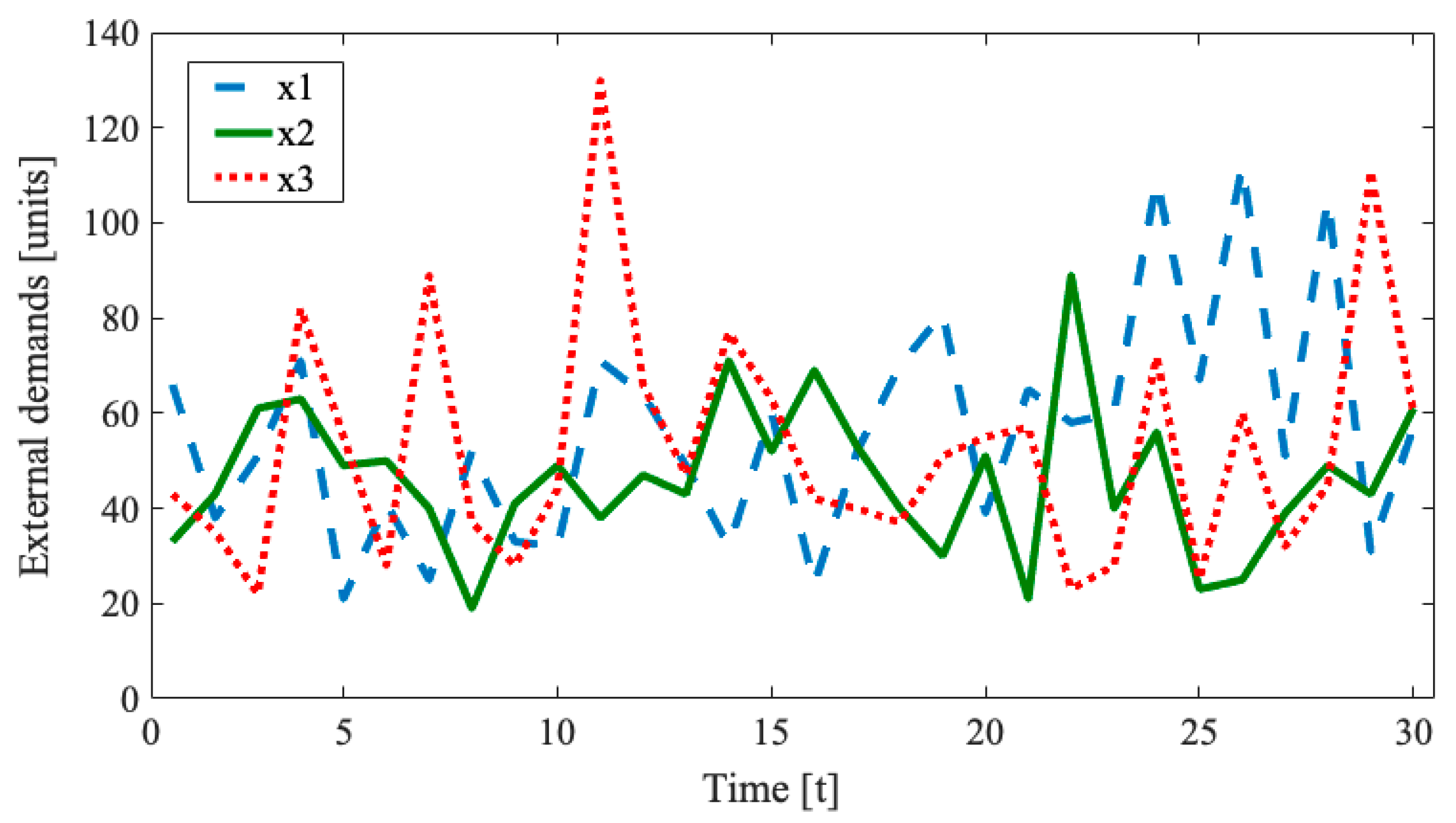
In this case, the external demand is generated using gamma distribution with the values rounded to the nearest integer. Figure 5 shows the demand requests that the controlled nodes aim to fulfill.

The baseline TIL vector [1156, 920, 496] units results in the holding cost equals to 4.7 × 10⁴. The optimization process in the 728th generation allows one to find the optimal TIL vector [474, 409, 256] units, which satisfies the external demands in full. The network costs are reduced to 5.5 × 10³. The resource flow is illustrated in Figure 6. It indicates that for both slowly and rapidly varying demand, the optimization process allows one to reduce the excess resources stored in the node warehouses.

4.2. Medium Network N–2

Figure 7 presents the topology of network N–2 and

Table A1. Attributes of node interconnections in network N–2.

From\To	1	2	3	4	5	6	7	8	9
1	-	-	0.7, 1	-	0.7, 3	-	-	-	-
2	-	-	-	-	-	0.6, 5	-	-	-
3	-	-	-	0.1, 5	-	-	-	-	-
4	0.3, 3	0.3, 3	-	-	-	-	-	-	-
5	-	0.3, 4	-	-	-	0.1, 3	-	-	-
6	0.4, 2	-	-	-	-	-	-	-	-
7	0.3, 5	-	0.1, 3	0.8, 4	0.1, 5	-	-	-	-
8	-	0.4, 1	-	0.1, 4	-	0.3, 4	-	-	-
9	-	-	0.2, 2	-	0.2, 1	-	-	-	-

lists the interconnection details. Due to increased structural complexity of this network and the next one, the visualization of the external demand and on-hand stocks using charts is not readable. Instead, the numerical data will be presented.

4.2.1. Results for Poisson Demand

The generated demand is in the range [2, 20] units. Using its highest value for each controlled node, the initial TIL vector is established as [231, 127, 57, 216, 123, 232] units and yields the storage costs of 1.6 × 10⁴. In this case, the full-search algorithm needs to check over 10¹³ candidate solutions. GA-based optimization reduces the costs to less than 10³ by finding the optimal solution—${\mathit{x}}_{\mathrm{optimum}}^{\mathit{T}}$ = [101, 37, 35, 98, 59, 99]—in the 13254th generation, i.e., after calculating 6.6 × 10⁵ potential solutions.

4.2.2. Results for Gamma Demand

The gamma distribution-based external demands belong to the range [20, 123] units. The initial TIL vector determined for this demand is equal to [1491, 743, 360, 1347, 784, 1337] units and results in 1.13 × 10⁵ holding costs. The optimal TIL vector obtained in 33 generations equals [477, 233, 222, 500, 304, 537] units and decreases the costs to 8 × 10³. The full-search method with the granularity of one unit requires to perform about 5.5 × 10¹⁷ simulations to find the best solution.

4.3. Large Network N–3

Figure 8 presents the interconnection structure of network N–3, which is yet more complex than the previously discussed ones.

Table A2. Attributes of node interconnections in network N–3.

From\To	1	2	3	4	5	6	7	8	9	10	11	12	13	14	15	16	17	18	19	20
1	-	0.7, 4	-	-	-	-	-	0.2, 3	0.8, 1	0.4, 2	-	-	-	-	0.3, 5	-	-	-	-	-
2	-	-	-	-	-	-	0.8, 2	-	-	0.3, 4	-	-	-	-	-	-	-	-	-	-
3	-	-	-	0.2, 4	-	-	-	-	-	-	-	0.4, 2	-	-	0.1, 4	-	-	-	-	-
4	-	-	-	-	-	-	0.1, 1	-	-	-	-	-	-	-	-	-	-	-	-	-
5	-	-	-	-	-	-	-	0.2, 5	-	-	-	-	-	-	-	-	-	-	-	-
6	0.6, 4	-	-	-	-	-	-	-	-	-	-	-	0.3, 2	-	-	-	-	-	-	-
7	-	-	-	-	-	-	-	-	-	-	0.2, 2	-	-	-	-	-	-	-	-	-
8	-	-	-	-	-	-	-	-	0.1, 5	-	-	-	-	-	-	-	-	-	-	-
9	-	-	-	-	-	0.4, 2	-	-	-	-	-	-	-	0.8, 5	-	-	-	-	-	-
10	-	-	-	-	-	-	-	-	-	-	0.6, 1	-	0.2, 2	-	-	-	-	-	-	-
11	0.3, 1	-	-	-	-	-	-	-	0.1, 5	-	-	-	-	0.1, 2	-	-	-	-	-	-
12	-	0.2, 5	-	-	-	-	-	-	-	-	-	-	-	-	-	-	-	-	-	-
13	-	-	0.5, 1	0.3, 5	-	-	-	-	-	-	-	-	-	-	-	-	-	-	-	-
14	-	-	-	-	-	-	-	-	-	-	-	-	-	-	-	-	-	-	-	-
15	-	-	-	0.5, 1	0.1, 3	0.3, 1	0.1, 1	-	-	-	0.2, 1	-	-	-	-	-	-	-	-	-
16	0.1, 3	-	0.2, 1	-	-	-	-	0.6, 1	-	-	-	0.3, 2	-	0.1, 4	-	-	-	-	-	-
17	-	-	-	-	-	0.3, 1	-	-	-	0.3, 5	-	0.3, 5	-	-	0.6, 3	-	-	-	-	-
18	-	-	-	-	0.4, 5	-	-	-	-	-	-	-	-	-	-	-	-	-	-	-
19	-	0.1, 3	-	-	-	-	-	-	-	-	-	-	0.5, 1	-	-	-	-	-	-	-
20	-	-	0.3, 4	-	0.5, 2	-	-	-	-	-	-	-	-	-	-	-	-	-	-	-

groups the attributes of links between the nodes. The external demands are imposed on all the controlled nodes.

4.3.1. Results for Poisson Demand

The baseline setting for the optimization process leads to the holding costs equal to 5.9 × 10⁴ with TIL vector calculated from (9) as:

$${\mathit{x}}_{\mathrm{initial}}^{\mathit{T}}=\left[ \begin{array}{c}789,333,126,74,97,368,90,84,\\ 245, 357, 196, 122, 114, 86, 455\end{array} \right]\mathrm{units}.$$

(12)

The GA-based optimization needs 5403 generations to approach the optimal solution that reduces costs related to the inventory storage to 3 × 10³. It is not feasible to find the best solution using the full-search algorithm, as it would involve running 6.2 × 10³³ simulations. The optimal TIL vector is obtained as:

$${\mathit{x}}_{\mathrm{optimum}}^{\mathit{T}}=\left[ \begin{array}{c}112,158,36,55,61,77,58,53\\ 120, 91, 76, 73, 36, 77, 153\end{array} \right]\mathrm{units}.$$

(13)

4.3.2. Results for Gamma Demand

Similarly as in the previous cases, the external demands generated using gamma distribution are characterized by greater uncertainty than the Poisson-based ones. The initial holding cost for the vector

$${\mathit{x}}_{\mathrm{initial}}^{\mathit{T}}=\left[ \begin{array}{c}4883,2264,771,530,509,2221,622,546,\\ 1521, 2046, 1163, 702, 683, 545, 2712\end{array} \right]\mathrm{units}$$

(14)

equals 4.2 × 10⁵. In the analyzed case, there are 4.45 × 10⁴⁵ candidate solutions for the TIL vector to consider. The GA-based optimization selected the TIL vector that leads to reducing the holding costs to 1.9 × 10⁴ (less than 5% of the initial state) in just 1394th generation, i.e., it needs to perform less than 7 × 10⁴ simulations. The best TIL vector is

$${\mathit{x}}_{\mathrm{optimum}}^{\mathit{T}}=\left[ \begin{array}{c}846,537,310,497,290,334,473,258,\\ 123, 578, 648, 323, 288, 393, 407\end{array} \right]\mathrm{units}.$$

(15)

Figure 9 presents the course of the fitness function changes as the optimization process evolves for network N–3. The dashed red line highlights the best solution evaluated using the parallel full-search algorithm.

To sum up, the presented numerical studies demonstrate the efficiency of the simulation-based optimization of logistic networks assisted by a continuous-domain GA algorithm. The external demands, which in practical settings considered here are not known a prori, lead to large search space of candidate solutions for any realistic logistic structure. Even with the hardware capabilities of today’s computers, it is not possible to perform the full-search operation for sophisticated architectures. The AI method applied in this work permits obtaining a solution close to the best one in a significantly shorter time.

5. Conclusions

The paper investigates the application of simulation-based optimization in order to improve the effectiveness of goods reflow in distribution networks with mesh-type architectures. The class of networks under consideration are influenced by uncertain exogenous demand. The resource redistribution is governed using an order-up-to inventory management strategy implemented in a networked manner. The optimization process based on continuous GA adjusts the policy parameters to the logistic system under consideration. The GA-based optimization provides a target inventory level so that a balance between two partially conflicting objectives—holding cost reduction and maintaining high customer satisfaction—is obtained. The numerical studies, assuming various system scales and external demands generated using different stochastic distributions, demonstrate the effectiveness of both the considered policy and GA as tools for AI-assisted optimization of modern logistic systems. Moreover, the analyzed cases indicate that the bigger the connection complexity, the greater the benefit of application of GA-based optimization in comparison to the full-search methods.

References

- Gereffi, G.; Frederick, S. The global apparel value chain, trade and the crisis: Challenges and opportunities for developing countries. World Bank Pol. Res. Work. Pap. 2010, 5281. [Google Scholar] [CrossRef]
- Berger, T.; Frey, C.B. Industrial renewal in the 21st century: Evidence from US cities. Reg. Stud. 2015, 50, 1–10. [Google Scholar] [CrossRef]
- Grazia Speranza, M. Trends in transportation and logistics. Eur. J. Oper. Res. 2018, 264, 830–836. [Google Scholar] [CrossRef]
- Sagiroglu, S.; Sinanc, D. Big data: A review. In Proceedings of the 2013 International Conference on Collaboration Technologies and Systems, San Diego, CA, USA, 20–24 May 2013; pp. 42–47. [Google Scholar] [CrossRef]
- Waller, M.A.; Fawcett, S.E. Data science, predictive analytics, and Big data: A revolution that will transform supply chain design and management. J. Bus. Logist. 2013, 34, 77–84. [Google Scholar] [CrossRef]
- Wang, G.; Gunasekaran, A.; Ngai, E.W.T.; Papadopoulos, T. Big data analytics in logistics and supply chain management: Certain investigations for research and applications. Int. J. Prod. Econ. 2016, 176, 98–110. [Google Scholar] [CrossRef] [Green Version]
- Ahmed, E.; Yaqoob, I.; Hashem, I.A.T.; Khan, I.; Ahmed, A.I.A.; Imran, M.; Vasilakos, A.V. The role of big data analytics in Internet of Things. Comput. Netw. 2017, 129, 459–471. [Google Scholar] [CrossRef]
- Potó, V.; Somogyi, J.Á.; Lovas, T.; Barsi, Á. Laser scanned point clouds to support autonomous vehicles. Transp. Res. Proc. 2017, 27, 531–537. [Google Scholar] [CrossRef]
- Xu, K.; Evers, P.T. Managing single echelon inventories through demand aggregation and the feasibility of a correlation matrix. Comput. Oper. Res. 2003, 30, 297–308. [Google Scholar] [CrossRef]
- Ignaciuk, P.; Bartoszewicz, A. Linear-quadratic optimal control of periodic-review perishable inventory systems. IEEE Trans. Cont. Syst. Technol. 2012, 20, 1400–1407. [Google Scholar] [CrossRef]
- Garcia, C.A.; Ibeas, A.; Vilanova, R. A switched control strategy for inventory control of the supply chain. J. Process Contr. 2013, 23, 868–880. [Google Scholar] [CrossRef]
- Purnomo, H.D.; Wee, H.M.; Praharsi, Y. Two inventory review policies on supply chain configuration problem. Comput. Ind. Eng. 2012, 63, 448–455. [Google Scholar] [CrossRef]
- Ignaciuk, P. Discrete inventory control in systems with perishable goods—A time-delay system perspective. IET Control Theory A 2014, 8, 11–21. [Google Scholar] [CrossRef]
- Kim, C.O.; Jun, J.; Baek, J.K.; Smith, R.L.; Kim, Y.D. Adaptive inventory control models for supply chain management. Int. J. Adv. Manuf. Technol. 2005, 26, 1184–1192. [Google Scholar] [CrossRef]
- Ignaciuk, P. Nonlinear inventory control with discrete sliding modes in systems with uncertain delay. IEEE Trans. Ind. Inform. 2014, 10, 559–568. [Google Scholar] [CrossRef]
- Sun, L.; Zhou, Y. A knowledge-based tree-like representation for inventory routing problem in the distribution system of oil products. Procedia Comput. Sci. 2017, 112, 1683–1691. [Google Scholar] [CrossRef]
- Poppe, J.; Basten, R.J.I.; Boute, R.N.; Lambrecht, M.R. Numerical study of inventory management under various maintenance policies. Reliab. Eng. Syst. Saf. 2017, 168, 262–273. [Google Scholar] [CrossRef]
- Garcia-Herreros, P.; Agarwal, A.; Wassick, J.M.; Grossmann, I.E. Optimizing inventory policies in process networks under uncertainty. Comput. Chem. Eng. 2016, 92, 256–272. [Google Scholar] [CrossRef]
- Kulkarni, S.; Patil, R.; Krishnamoorthy, M.; Ernst, A.; Ranade, A. A new two-stage heuristic for the recreational vehicle scheduling problem. Comput. Oper. Res. 2018, 91, 59–78. [Google Scholar] [CrossRef]
- Ignaciuk, P.; Wieczorek, Ł. Optimization of mesh-type logistic networks for achieving max service rate under order-up-to inventory policy. Adv. Intell. Syst. Comput. 2018, 657, 118–127. [Google Scholar] [CrossRef]
- Ignaciuk, P. Dynamic modeling and order-up-to inventory management in logistic networks with positive lead time. In Proceedings of the 2015 IEEE International Conference on Intelligent Computer Communication and Processing (ICCP), Cluj-Napoca, Romania, 3–5 September 2015; pp. 507–510. [Google Scholar] [CrossRef]
- Simon, D. Evolutionary Optimization Algorithms; John Wiley & Sons: Hoboken, NJ, USA, 2013; ISBN 978-0470937419. [Google Scholar]
- Wieczorek, Ł.; Ignaciuk, P. Intelligent Support for Resource Distribution in Logistic Networks Using Continuous-Domain Genetic Algorithms. In Proceedings of the 2018 IEEE Second International Conference on Data Stream Mining & Processing, Lviv, Ukraine, 21–25 August 2018; pp. 424–429. [Google Scholar] [CrossRef]
Figure 1.
Node routine sequence.
Figure 2.
Resource distribution network N–1.