Residential Power Traces for Five Houses: The iHomeLab RAPT Dataset

Abstract

Datasets with measurements of both solar electricity production and domestic electricity consumption separated into the major loads are interesting for research focussing on (i) local optimization of solar energy consumption and (ii) non-intrusive load monitoring. To this end, we publish the iHomeLab RAPT dataset consisting of electrical power traces from five houses in the greater Lucerne region in Switzerland spanning a period from 1.5 up to 3.5 years with a sampling frequency of five minutes. For each house, the electrical energy consumption of the aggregated household and specific appliances such as dishwasher, washing machine, tumble dryer, hot water boiler, or heating pump were metered. Additionally, the data includes electric production data from PV panels for all five houses, and battery power flow measurement data from two houses. Thermal metadata is also provided for the three houses with a heating pump.

Dataset: DOI: 10.5281/zenodo.3581895

Dataset License: CC-BY

1. Summary

Datasets with measurements of the domestic energy breakdown per appliance are of interest from different perspectives. Firstly, there is an ever-increasing amount of renewable electrical energy production and with that, a growing interest in solutions that can handle its stochastic nature such as demand response [1,2], optimized self-consumption [3] or smart energy trading [4]. Datasets that measure the consumption of aggregate households, as well as the (major) appliances, are required to base the development of such solutions on actual data. Secondly, datasets consisting of domestic electrical energy consumption with an appliance breakdown are essential for the non-Intrusive Load Monitoring (NILM) research, which aims at disaggregating the domestic energy consumption on device-level [5,6]. Finally, the data can also be useful for example in research in the domains of energy usage prediction, energy usage feedback systems, time-series data analysis and processing, and consumer behavior.

Our motivation in publishing this work is primarily to extend the list of available open datasets and therefore foster innovation in the corresponding fields. Our dataset consists of electrical power traces from five houses in the greater Lucerne region in Switzerland spanning a period from 1.5 up to 3.5 years. For each house, the electrical energy consumption of the aggregated household and specific appliances such as dishwasher, washing machine, tumble dryer, hot water boiler, or heating pump were metered. The data includes additional electric production data from PV panels for all five houses, and power flow measurement data from a battery in the case of two houses. Three houses had a heating pump installed. For these houses, thermal metadata is also provided in order to enable corresponding simulations.

The dataset collection started in the framework of the project Wizard for the optimal management of Electrical Energy in a prosumer household (WizEE) [7] and is ongoing in the project Swiss Competence Center for Energy Research, Future Energy Efficient Buildings and Districts (SCCER FEEB&D) [8]. We, therefore, plan to release further data in the future. Based on the collected data, the authors investigated how well algorithms can predict the usage of domestic appliances solely based on historic electrical energy consumption data [9].

Relation to Other Datasets

A recent and comprehensive overview of datasets that have been used for load disaggregation work can be found e.g., in [10]. The dataset most similar to ours is named ECO [11] standing for Electricity Consumption and Occupancy dataset. It stems also from Switzerland and comprises a similar number of houses and duration. The main differences are the sampling frequency, 1 Hz in case of the ECO and 5 min for the presented dataset, and submetered devices. Our dataset includes data of appliances that consume a major fraction of the electrical household energy, i.e., heat pump and hot water boilers, but also photovoltaic production and household battery power flow measurements. The Dataport [12] database containing data from over 1000 residential homes is the most notable source of data that includes measurement of such heavy power consuming appliances. Available metering data stems however all from the US with quite distinct appliances and electrical installations compared to Switzerland. To our knowledge, datasets containing electrical power measurements with a similar breadth as Dataports are only available from the Irish Commission of Energy Regulation [13] and the ‘Building Data Genome Project’ [14]. The former contains however only 30 min aggregated residential data whereas the latter only hourly aggregated non-residential data.

2. Data Description

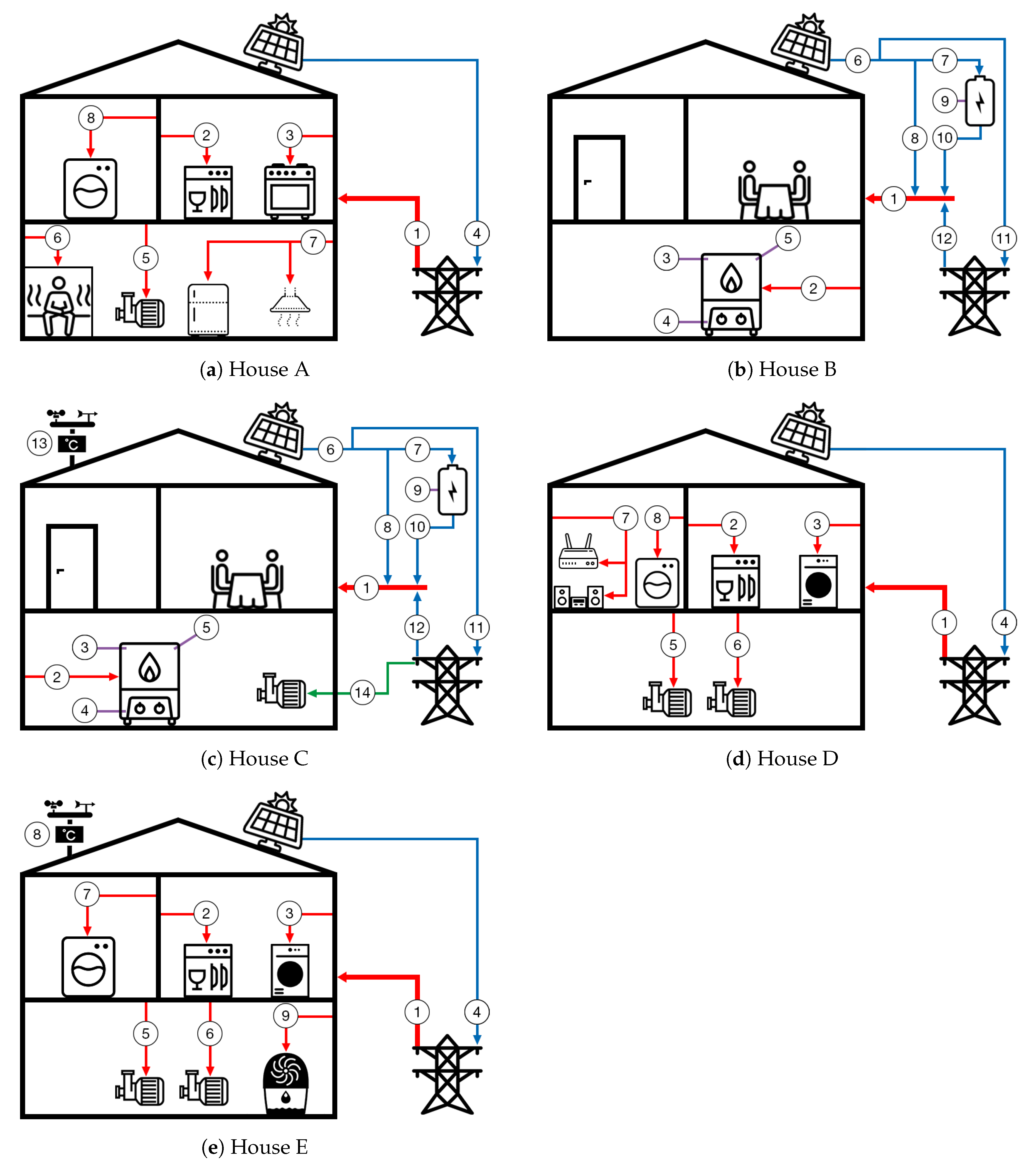
The dataset consists of data from five houses located in the greater Lucerne region. Each house is equipped with up to seven meters that measure each of the average consumed power per sampling period. Figure 1 contains a schematic overview of the installed (sub)metering and the corresponding wiring: The main meters of the houses are represented as thick red arrows. Thin red arrows indicate submetered appliances. Other electrical connections and corresponding meters are shown in blue/green. Sensor numbers are listed in

Table 1. List of sensors installed in the different houses. Numbers in column ‘#’ refer to those in Figure 1. ‘Sensor Name’ gives the name of the sensor as used in the data. ‘T${}_{orig}$’ indicates the original sampling rate. ‘M-id’ lists the meter identity as given in Table 5. Abbreviations: ‘pc’ stands for ‘power consumption’, ‘PV’ for ‘photovoltaic’, ‘ed’ for ‘event driven’.

#	Description	Sensor Name	Unit	T${}_{\mathbf{orig}}$	M-id
House A
1	total pc	A_total_cons_power	W	120 s	a
2	pc of dishwasher	A_dishwasher_power	W	120 s	b
3	pc of cooking, backing	A_stove_power	W	120 s	c
4	PV power production	A_exp_power	W	120 s	d,e 1
5	pc of heat pump	A_hp_power	W	120 s	f
6	pc of several devices: sauna, steam shower, outdoor lighting	A_sauna_power	W	120 s	c
7	pc of several devices: fridge, comfort ventilation, central vacuum cleaner	A_additional_power	W	120 s	b
8	pc of washing machine	A_washing_machine_power	W	120 s	f
House B
1	total pc	B_total_cons_power	W	300 s	g
2	pc of boiler	B_boiler_power	W	300 s	h
3	water boiler: temp. at the top	B_boilertemp_top	°C	300 s	i
4	water boiler: temp. at the bottom	B_boilertemp_bottom	°C	300 s	i
5	water boiler: on/off-status of heater 1, 2, 3 and thermostat 2	B_boiler_heater_*, B_boiler_on_thermostat	–	300 s ed	j
6	total PV power production	B_pv_prod_power	W	300 s	g
7	from solar panel to battery	B_to_batt_power	W	300 s	g
8	pc from solar panel directly	B_direct_cons_power	W	300 s	g
9	battery charge state (100% = full)	B_batt_state	%	300 s	g
10	pc from battery	B_from_batt_power	W	300 s	g
11	from solar panel in grid	B_to_net_power	W	300 s	g
12	pc from grid	B_from_net_power	W	300 s	g
House C
1	total pc	C_total_cons_power	W	120 s 3 300 s	a,g 3
2	pc of boiler	C_boiler_power	W	300 s	h
3	water boiler: temp. at the top	C_boilertemp_top	°C	300 s	i
4	water boiler: temp. at the bottom	C_boilertemp_bottom	°C	300 s	i
5	water boiler: on/off-status of heater 1, 2, 3, thermostat, relay, utility 2	C_boiler_heater_*, C_boiler_on_*	–	300 s ed	j
6	total PV power production	C_pv_prod_power	W	300 s	g
7	from solar panel to battery	C_to_batt_power	W	300 s	g
8	pc from solar panel directly	C_direct_cons_power	W	300 s	g
9	battery charging state (100% = full)	C_batt_state	%	300 s	g
10	pc from battery	C_from_batt_power	W	300 s	g
11	from solar panel in grid	C_to_net_power	W	300 s	g
12	pc from grid	C_from_net_power	W	300 s	g
	metering of solar radiation	C_solarlog_radiation	$\frac{\mathrm{W}}{{\mathrm{m}}^2}$	120 s	k
13	environmental data logged by weather station, see Table 3	C_weather_*	*	1 h	l
14	pc of heat pump	C_hp_power	W	120 s	a
14	ripple control signal for heat pump	C_hp_on_utility	-	ed	m
15	outdoor temperature next to sensor of heat pump	C_temperature_out	°C	120 s	i
House D
1	total pc	D_total_cons_power	W	120 s	a
2	pc of dishwasher	D_dishwasher_power	W	60 s	n
3	pc of tumble dryer	D_tumble_dryer_power	W	60 s	n
4	PV power production	D_exp_power	W	120 s	d
5	pc of heat pump	D_hp_power	W	300 s	o
6	pc of rainwater pump	D_rainwater_power	W	60 s	n
7	pc of HiFi system and router	D_audio_wlan_og_power	W	60 s	n
8	pc of washing machine	D_washing_machine_power	W	60 s	n
House E
1	total pc	E_total_cons_power	W	300 s	p
2	pc of dishwasher	E_dishwasher_power	W	60 s	n
3	pc of tumble dryer	E_tumble_dryer_power	W	60 s	n
4	PV power production	E_prod_power	W	300 s	p
5	pc of heating gas pump	E_gasheating_pump_power	W	60 s	n
6	pc of water pump of solar thermal collectors	E_solarheating_pump_power	W	60 s	n
7	pc of washing machine	E_washing_machine_power	W	60 s	n
8	environmental data logged by weather station, see Table 3	E_weather_*	*	1 h	l
9	pc of dehumidifier	E_dehumidifier_power	W	60 s	n

¹ Meter d was replaced with e on 2018-4-16.

² Please refer to Section 4.4 for the meaning of these sensors.

³ Meter a (T${}_{\mathrm{orig}}$ = 120 s) removed on the 2017-09-26. Meter g (T${}_{\mathrm{orig}}$ = 300 s) installed on 2017-11-01.

. The table contains also a description of the sensors and their denomination in the dataset. The dataset is stored in the Hierarchical Data Format (HDF) version 5 [15]. If using the Python programming language, it is easily accessible with pandas [16,17] via the ‘pandas.read_hdf(path/to/file)’ function. All timestamps are given in Swiss local time, i.e., UTC+1:00h during winter half-year (November to March) and UTC+2:00h during the summer half-year (April to October).

2.1. Electrical Power Data

Electrical power measurements are available in a raw and processed version. The raw sensor measurements are provided one HDF-file per sensor combined in one folder per house. The processed data is joined in one HDF-file per house as summarized in

Table 2. Summary of the presented dataset: Name of houses, corresponding Hierarchical Data Format (HDF)-files, sampling rate, available period and ‘short name’ of the relevant weather station of MetoSwiss for each house, see Section 2.2 for details.

Houses	File Name	Sampling Rate	Time Range	Weather Station
house A	datasets/dfA_300s.hdf	5 min	2017-04-01–2018-10-30	LUZ
house B	datasets/dfB_300s.hdf	5 min	2017-03-01–2019-07-31	MMSTA
house C	datasets/dfC_300s.hdf datasets/dfC_3600s.hdf	5 min 1 h (weather)	2015-11-30–2019-07-31	EGO
house D	datasets/dfD_300s.hdf	5 min	2016-04-23–2019-07-31	LUZ
house E	datasets/dfE_300s.hdf datasets/dfE_3600s.hdf	5 min 1 h (weather)	2016-12-01–2019-07-31	LUZ

. The table contains also the logged time span for each house. The HDF-files consist of tables where each tables’ column corresponds to one sensor reading.

For the processed power data, we down-sampled some of the measured sensor data to have a consistent sampling interval of 5 min across all sensors of the five houses. This was mostly done for sensors of houses A, D and E. The original sampling rate of each sensor is given in column $T_{orig}$ of Table 1.

2.2. Weather Data

Houses C and E were equipped with a local weather station. The corresponding sensor descriptions and names are listed in

Table 3. Description of the data recorded by the ‘My Weatherbox’ in houses C and E. The technical specification of the weather station can be found in Table 5, sensor l.

Description	Sensor Name	Unit	T${}_{\mathbf{orig}}$
House C
indoor humidity	C_weather_humidity_in	RH	3600 s
outdoor humidity	C_weather_humidity_out	RH	3600 s
outdoor pressure	C_weather_pressure	mbar	3600 s
indoor temperature	C_weather_temperature_in	°C	3600 s
outdoor temperature	C_weather_temperature_out	°C	3600 s
House E
indoor humidity	E_weather_humidity_in	RH	3600 s
indoor humidity in cellar	E_weather_humidity_cellar	RH	3600 s
outdoor humidity	E_weather_humidity_out	RH	3600 s
outdoor pressure	E_weather_pressure	mbar	3600 s
indoor temperature	E_weather_temperature_in	°C	3600 s
indoor temperature in cellar	E_weather_temperature_cellar	°C	3600 s
outdoor temperature	E_weather_temperature_out	°C	3600 s

. Sampling was done on an hourly basis. The available HDF-files are given in Table 2. As house D is in close proximity to E, corresponding outdoor weather data can be used for both.

For all houses, hourly averaged weather data can be obtained from the Swiss Federal Office of Meteorology and Climatology, MeteoSwiss, upon registration at https://gate.meteoswiss.ch/idaweb/login.do. This service is free of charge for educational and research purposes. The ‘short names’ of the relevant weather stations for each house are listed in Table 2.

2.3. Thermal Metadata

Houses A, C and D include the electrical consumption of the heat pump. To make the dataset also useful for research questions involving the thermal aspects of the heated buildings, relevant thermal characteristics of these three houses are provided in

Table 4. Thermal metadata of houses A, C and D.

	House A	House C	House D
Building Information
Description	Semi-detached house with three floors: The lowest floor of the southern facade is partially built into the hillside. The window area on the main northern facade (three floors) is small. The window area on the main southern facade (two floors) is large.	Detached house with 4 floors: only the topmost floor is freestanding. The rest of the north-east (NE) facade and around 1/3 of south-east and north-west facades are embedded in the hillside. The main facade is oriented towards south-west (SW). The heated volume includes an additional self-contained flat. No electrical consumption (except heat pump) origins from that flat.	Detached house with 2 floors: only the upper floor is freestanding, the complete NE and SW facades of the lower floor are embedded in the hillside. The main facades are oriented towards NE and SW.
Inhabitants	three-person household	four-person household + one person in flat	five-person household
Heated space [m${}^2$]	146	295	218
Building envelope	Construction year: 2005, one-shell brickwork, 16 cm Isolation	Construction year: 2005, two-shell brickwork: outer: 15 cm brick, insulation: 14 cm, flumroc.ch ’Dämmplatte 1’, thermal conductivity: 0.035 W/mK, inner: 15 cm brick	Construction year: 2008, ground floor concrete, first floor 80 mm massive wood construction encased in 260–300 mm insulation. Energy balance according to SAI 380/1 (2007) 33 kWh/m${}^2$ year. See also Section 4.4
Windows	double glazing, heat transmission coefficient: 1.9 W/(m${}^2$ K)	double glazing, heat transmission coefficient: 1.9 W/(m${}^2$ K)	triple glazing
Heat Pump Information
Comments	Heat pump has two compressors, one is used for domestic hot water (60 °C), the other for space heating (30–35 °C).	Heat pump is only used for space heating. Domestic hot water is generated in a conventional hot water boiler.	Heat pump has two compressors, one is used for domestic hot water (60 °C), the other for space heating (35–40 °C).
Heat pump specs	Manufacturer: KWT (acquired by Viessmann), Model: Swissline 28NHB, Type: Sole—Wasser	Manufacturer: Stiebel Eltron, Model: WPL 23, Type: air–water	Manufacturer: alpha-innotec, Model: SWC 60H, Type: sole–water
Emitter type	floor heating	floor heating	floor heating
Ripple controlled heat pump	No	Yes	No

.

3. Methods

3.1. Measurement Equipment and Data Collection

Metering was done with the sensors listed in

Table 5. List of employed measurement equipment. Indexes given in column meter id ‘M-id’ are used in Table 1. The S0 interface is defined in IEC standard 62053-31 and DIN standard 43 864.

M-id	Device Name	Details
a	L+G ZMD120AP	Meter installed by utility. Readout of pulse output (S0): 1000 impulses/kWh.
b	MCI single-phase	Readout of pulse output (S0): 1000 impulses/kWh.
c	ABB OD4165	Readout of pulse output (S0): 100 impulses/kWh.
d	L+G E350	Readout of pulse output (S0): 1000 impulses/kWh.
e	Elster AS3000	Readout of pulse output (S0): 1000 impulses/kWh.
f	Voltcraft DPM-314D	Readout of pulse output: 1000 impulses/kWh.
g	Fronius Symo Hybrid 5.0-3-S	Inverter from Fronius (www.fronius.com) with an integrated logging system to monitor the various power flows through the device.
h	RPi Boiler Control Unit	Custom made boiler control unit implemented on a Raspberry Pi that switches the three individual heating elements of the boiler. The boiler_power is calculated based on the configured value of the nominal consumption of the switched-on heating elements. The control logic is documented in Section 4.4, house B.
i	Temp. Sensor DS1820	1-wire bus temperature sensor DS1820
j	Switch State Sensor	Sensor is connected to RPi Boiler Control unit. The information on the voltage drop over the switch is transformed in a binary state signal.
k	Tritec Spektron 320	Soloar irradiation sensor from Tritec (www.tritec-energy.com). Measuring range 0-1500 W/m${}^2$. Accuracy $\pm 5$% annual mean. Considering an area and efficiency of a solar panel, the output of the sensor can be used to calculate the generated power of a corresponding installation.
l	TFA My Weatherbox	Weather station from TFA (www.tfa-dostmann.de). Temperature sensors–accuracy: $\pm 1$ °C; humidity sensor–resolution: 1% RH, accuracy: $\pm 5$% RH.
m	Ripple Control	Ripple control signal as obtained from the utility company.
n	myStrom WiFi Switch (CH)	Smart plug from myStrom (mystrom.ch). Measuring range 2–2300 W. Accuracy $\pm <1$%.
o	Hager EC311	Readout of pulse output (S0): 10 impulses/kWh.
p	Solar-Log 1200	Monitoring and energy management system from Solar-Log (www.solar-log.com). It includes options to export data.

. In cases where the number of pulses from the S0 interfaces per capturing period was counted, the measuring method induces the uncertainty that a major fraction of the energy of the first pulse in a capturing period could actually have been consumed before that period. One consequence thereof is that even if the actual energy consumption of an appliance was constant, the measured signal could exhibit a variation ≤ $(\mathrm{energy}/\mathrm{pulse})$.

The data collection infrastructure is visualized in Figure 2: Measurements were collected in files directly by the myStrom WiFi Switches, the Fronius Symo Hybrid, and the Weatherbox. All other sensors were read-out by means of a Raspberry Pi (www.raspberrypi.org) and the collected data was then uploaded to an FTP server. All raw measurement files were finally imported into a database with custom scripts.

3.2. Processing of Raw Data

Multiple sensors in our dataset sampled with a higher frequency than once per five minutes and some sensors for the boilers of houses B and C were both event-driven and sampling at regular intervals. In order to provide an easily accessible dataset, we decided to publish a pre-processed dataset alongside the raw data. The corresponding code is available under https://github.com/ihomelab/RAPT-dataset. The pre-processing included the following steps:

• Round timestamps for the respective capture period, e.g., rounding ‘2018-10-01 18:05:08’ to ‘2018-10-01 18:05:00’
• Convert electrical meter measurements to mean consumed power ([W]) per period.
• Linearly interpolate missing data for periods up to 15 min.
• Down-sample everything to a capture period of 5 min using the mean, except for the weather data, where an hourly resolution was kept.
• Calculate boiler_power: the boiler_power is calculated (not measured) in the RPi Boiler Control Unit, see sensor h in Table 5. Switch-on times are provided as sensors C_boiler_heater_1\2\3. As these sensors were also event-driven, the energy consumption was redistributed on the regular capture period of 5 min during pre-processing.

4. Usage Notes

4.1. Reading the Dataset

Reading the dataset in Python is straightforward. Using the Python package pandas [16], HDF files can be read with read_hdf(...), as an example:

• import pandas as pd
• pathToHouseA = "datasets/dfA_300s.hdf"
• dfA_300s = pd.read_hdf(pathToHouseA)

dfA_300s refers to a standard pandas DataFrame with the timestamp as index and available meters as columns.

4.2. Missing Data

Due to connection issues, reconstruction, and technical issues, the dataset contains missing data. It is stored as NaN. Figure 3 summarizes the corresponding information for the dataset (some weather sensors with similar missing data patterns were omitted). The different dates where logging started for the houses are easily observable. More detailed heat plots of the houses, showing the percentage of missing data per three days is provided alongside the data.

Using pandas DataFrames, the missing data can be easily extracted by df[df[‘sensor_name’].isnull()].index where df is the pandas DataFrame and ‘sensor_name’ is the name of the respective sensor as a string. Additionally, we extracted the start and end dates of missing data for all the sensors and stored them in CSV files missingData/<sensorName>.csv. These files are provided alongside the data.

4.3. Known Issues

A simple sanity check of the measured data consists of testing that the sum of all measured appliances must always be smaller or equal to the total consumed energy. In the case of houses B and C, there is a small portion of samples where this condition is not met, 0.07% and 0.28% respectively. These cases are mostly small deviations that can be attributed to the normalization of the data during the pre-processing steps, see Section 3.2.

4.4. Particularities of the Installations and Corresponding Data

House B

• Houses B has a solar panel, battery and a hot water boiler. The latter two are controlled by a custom controller, see sensor h in Table 5: If (B_pv_prod_power - B_total_cons_power) > 600 W, the B_boiler_heater_* are controlled according to the logic below:
• Daytime rules, i.e. high electrical tariff

  -

  ifboiler_on_thermostat == off then boiler_heater_* = off

  -

  ifboiler_on_thermostat == on and (boilertemp_top $<T_{min}$ or boilertemp_bottom $<T_{min}$) then boiler_heater_* = on

  -

  if (boilertemp_top $>T_{min}$ and boilertemp_bottom > $T_{min}$) and (batt_state $\le 85$%) then boiler_heater_* = off

  -

  if (boiler_on_thermostat == ’on’) and batt_state > 85% and boilertemp_top$<T_{max}$ and boilertemp_bottom$<T_{max}$ then boiler_heater_* = on

• Night-time rules, i.e., low electrical tariff

  -

  ifboiler_on_thermostat == on and boilertemp_top$<T_{minnight}$ then boiler_heater_* = on

  -

  ifboilertemp_top$>T_{maxnight}$thenboiler_heater_* = off

  Here, T${}_{min}=40$ °C, T${}_{max}=65$ °C and T${}_{minnight}=35$ °C, T${}_{minnight}=45$ °C. Depending on the current photovoltaic production, the three heating elements boiler_heater_1/2/3 are individually switched on. Remaining power will, in all cases, be used to charge the battery to its maximum. Further excess power is only after that allowed to flow back into the electrical grid.
• Installed battery: ‘Fronius Solar Battery 6.0’ from Fronius (www.fronius.com): Usable capacity of the battery: 4800 Wh, nominal discharging and charging power 3200 W.

House C

• The family inhabiting house C was on an extended leave from 2016-06-24 until 2016-08-13 with corresponding low power consumption in that period.
• The heat pump of house C is directly connected to the electrical grid that means the corresponding power is not subsumed in C_total_cons_power. In exchange for a lower electrical tariff, the utility has the right to control switch-on times of the heat pump by means of ripple control. Before the 2016-04-01, the utility inhibited switch-on with minor exception from 11 to 12 o’clock, 15 to 18 o’clock and from 22 to 2 o’clock the following morning. Starting with the 2016-04-01, the utility is allowed to variably block the heat pump, where each blocked period has to be followed by a period of equal or longer duration within which the heat pump is allowed to pull power. The ripple control signal has been obtained from the utility and is available as sensor C_hp_on_utility, a value of 1 indicating the pump is allowed to pull power.
• Heating of the hot water boiler was controlled in the following ways:

  -

  Before 2016-10-17: The boiler heating is turned on if the following signals are in the ‘on’ status: C_boiler_on_utility and C_boiler_on_thermostat. The former corresponds to the ripple control signal from the utility and the latter indicates if the water temperature in the boiler is below a certain threshold. The sensor C_boiler_on_relais is irrelevant for this period.

  -

  Between 2016-10-17 and 2017-01-23: The boiler heating is turned on if in addition to C_boiler_on_utility and C_boiler_on_thermostat, the signal C_boiler_on_relais is also in status ’on’. The signal C_boiler_on_relais is switched according to the following logic: (i) ’on’ if C_boilertemp_top < 42 °C (ii) ’off’ if C_boilertemp_top > 48 °C (approximately every 14 days the threshold was manually set to 60 °C).

  -

  Between 2017-01-23 and 2017-10-11: Due to recurrent difficulties with the more advanced control, the logic was switched back to the one used before 2016-10-17, see above.

  -

  After 2017-10-15: After the retrofit, see below, battery charging and boiler heating is controlled by a custom controller, see sensor h in Table 5: If (C_pv_prod_power - C_total_cons_power) > 900 W, the C_boiler_heater_* are controlled according to the logic as described for house B with the following difference. In case the boiler is charged during the night, battery discharging is disallowed. The sensor C_boiler_on_relais is irrelevant for this period.

• 2017-09-26: Established electrical connection of new photovoltaic panels.
• 2017-11-29: Connected new battery to power system. The battery type is identical as for house B, see corresponding specifications.
• The installations of PV panels and battery had the following consequences on the electrical installation:

  -

  Before the PV installation, the solar irradiation was logged with a solar irradiation sensor Tritec Spektron 320, see Table 5. The corresponding sensor is called C_solarlog_radiation and is only available until the retrofit.

  -

  After the retrofit, electrical power consumption from the boiler was calculated by the RPi Boiler Control Unit, see sensor h in Table 5. This sensor was not available before. The power consumption level of the boiler before the retrofit did however not vary because heating elements were always jointly turned on. The consumed power can be indirectly deduced from the power steps in the aggregate signal.

House D

• The house is constructed as a “Zero-energy home”—Minergie-P, see Minergie (www.minergie.ch). That means that calculated heating energy per inhabited square meter and year amounts to 33 kWh.
• Solar panels have been disconnected between 2017-07-14 and 2017-10-18 because panels were exchanged. The area and exposition of the installed panels did not change but due to the improved efficiency, peak power changed from 8.14 kW to 10.45 kW.

House E

• A new dishwasher has been installed on the 2017-09-01.
• A new washing machine has been installed on the 2017-12-15
• The dehumidifier is located in the cellar. Its control logic ensures that the cellar is dehumidified at all times while maximizing the usage of excess solar power to this end. That means that every 10 min, the control logic checks if the relative humidity in the cellar exceeds an upper or falls below a lower limit and switches the dehumidifier on or off, respectively. Depending on the situation, different limits are applied. The limits are listed in

  Table 6. Situation dependent upper and lower limits employed in the control logic of the dehumidifier of house E.

  Situation	Lower Limit [RH]	Upper Limit [RH]
  (B_pv_prod_power - B_total_cons_power) > 600 W (nominal power of dehumidifier)	48	53
  high electrical tariff (starting at 6 am)	58	63
  low electrical tariff (starting at 10pm)	53	58

  .

References

- Siano, P. Demand Response and Smart Grids—A Survey. Renew. Sustain. Energy Rev. 2014, 30, 461–478. [Google Scholar] [CrossRef]
- Birrer, E.; Picard, C.; Huber, P.; Bolliger, D.; Klapproth, A. Demand Response Optimized Heat Pump Control for Service Sector Buildings–A Modular Framework for Simulation and Building Operation. Comput. Sci. Res. Dev. 2017, 32, 25–34. [Google Scholar] [CrossRef]
- Luthander, R.; Widén, J.; Nilsson, D.; Palm, J. Photovoltaic Self-Consumption in Buildings: A Review. Appl. Energy 2015, 142, 80–94. [Google Scholar] [CrossRef] [Green Version]
- Kok, K. The PowerMatcher: Smart Coordination for the Smart Electricity Grid. Ph.D. Thesis, Technical University of Denmark, Kgs. Lyngby, Denmark, July 2013. [Google Scholar]
- Hart, G.W. Nonintrusive Appliance Load Monitoring. Proc. IEEE 1992, 80, 1870–1891. [Google Scholar] [CrossRef]
- Zeifman, M.; Roth, K. Nonintrusive Appliance Load Monitoring: Review and Outlook. IEEE Trans. Consum. Electron. 2011, 57, 76–84. [Google Scholar] [CrossRef]
- WizEE–Wizard for the Optimal Management of Electrical Energy in a Prosumer Household. Available online: https://www.aramis.admin.ch/Grunddaten/?ProjectID=37341 (accessed on 30 January 2020).
- Swiss Competence Center for Energy Research SCCER FEEB&D of the Swiss Innovation Agency Innosuisse. Available online: https://www.sccer-feebd.ch (accessed on 30 January 2020).
- Huber, P.; Gerber, M.; Rumsch, A.; Paice, A. Prediction of Domestic Appliances Usage Based on Electrical Consumption. Energy Inform. 2018, 1, 16. [Google Scholar] [CrossRef] [Green Version]
- Murray, D.; Stankovic, L.; Stankovic, V. An Electrical Load Measurements Dataset of United Kingdom Households from a Two-Year Longitudinal Study. Sci. Data 2017, 4, 1–12. [Google Scholar] [CrossRef] [PubMed] [Green Version]
- Beckel, C.; Kleiminger, W.; Cicchetti, R.; Staake, T.; Santini, S. The ECO Data Set and the Performance of Non-intrusive Load Monitoring Algorithms. In Proceedings of the 1st ACM Conference on Embedded Systems for Energy-Efficient Buildings, Memphis, TN, USA, 4–6 November 2014. [Google Scholar] [CrossRef]
- Dataport. Available online: https://dataport.pecanstreet.org/ (accessed on 29 January 2020).
- Archive, I.S.S.D. Home, Irish Social Science Data Archive. Available online: https://www.ucd.ie/issda/data/commissionforenergyregulationcer/ (accessed on 18 January 2019).
- Miller, C.; Meggers, F. The Building Data Genome Project: An Open, Public Data Set from Non-Residential Building Electrical Meters. Energy Procedia 2017, 122, 439–444. [Google Scholar] [CrossRef]
- The HDF Group. Hierarchical Data Format Version 5. Available online: https://www.hdfgroup.org (accessed on 30 January 2020).
- McKinney, W. Data Structures for Statistical Computing in Python. In Proceedings of the 9th Python in Science Conference, Austin, TX, USA, 28 June–3 July 2010. [Google Scholar]
- Python Data Analysis Library—Pandas: Python Data Analysis Library. Available online: https://pandas.pydata.org (accessed on 21 January 2019).
Figure 1.
Schematic overview of installed meters and corresponding wiring: The main meters of the houses are represented as thick red arrows. Thin red arrows indicate submetered appliances. Other electrical connections and corresponding meters are shown in blue/green. The description for the sensor number is available in Table 1.
Figure 2.
Overview of how the data was collected in general.
Figure 3.
Heatplot of missing data for all houses (some weather sensors are omitted). The heatplot shows the percentage of missing data per month, i.e., 1 means no data (dark regions) and 0 means all data (brighter regions) is available.