Applying Eye Tracking with Deep Learning Techniques for Early-Stage Detection of Autism Spectrum Disorders

Abstract

Autism spectrum disorder (ASD) poses a complex challenge to researchers and practitioners, with its multifaceted etiology and varied manifestations. Timely intervention is critical in enhancing the developmental outcomes of individuals with ASD. This paper underscores the paramount significance of early detection and diagnosis as a pivotal precursor to effective intervention. To this end, integrating advanced technological tools, specifically eye-tracking technology and deep learning algorithms, is investigated for its potential to discriminate between children with ASD and their typically developing (TD) peers. By employing these methods, the research aims to contribute to refining early detection strategies and support mechanisms. This study introduces innovative deep learning models grounded in convolutional neural network (CNN) and recurrent neural network (RNN) architectures, employing an eye-tracking dataset for training. Of note, performance outcomes have been realised, with the bidirectional long short-term memory (BiLSTM) achieving an accuracy of 96.44%, the gated recurrent unit (GRU) attaining 97.49%, the CNN-LSTM hybridising to 97.94%, and the LSTM achieving the most remarkable accuracy result of 98.33%. These outcomes underscore the efficacy of the applied methodologies and the potential of advanced computational frameworks in achieving substantial accuracy levels in ASD detection and classification.

1. Introduction

A neurodevelopmental condition known as autism spectrum disorder (ASD) is characterised by differences in neurological functioning. People who are diagnosed as autistic might exhibit a variety of behavioural patterns, interests, and behaviours such as engaging in repetitive behaviours or exhibiting a strong fixation on specific objects. People with ASD may have trouble communicating and interacting with others. Furthermore, it is important to point out that people with ASD may exhibit different learning and attention patterns from typically developing people. There is a notable global increase in the prevalence of autism spectrum disorder, with a continuous annual rise in the number of individuals diagnosed with this neurodevelopmental disorder. According to the Centre for Disease Control and Prevention (CDC), the prevalence of ASD among 8-year-olds in the United States is 1 in 36. According to data from the autism and developmental disabilities monitoring (ADDM) network, the percentage of children diagnosed with ASD at age 8 increased by 100 percent between 2000 and 2020 (Maenner, et al., 2023 [1]). For this reason, the importance of early ASD detection lies in its capacity to expedite precise diagnoses, thus enabling timely interventions during critical developmental stages. This temporal alignment enhances the effectiveness of therapeutic protocols and educational interventions. Moreover, the early identification of ASD creates a foundation for families to avail themselves of specialised services and engage with support networks, subsequently enhancing the development trajectory of affected children. Importantly, support groups serve as crucial resources for families navigating the challenges posed by Autism, offering advice, collective wisdom, and emotional reinforcement (Øien; Salgado-Cacho; Zwaigenbaum, et al. [2,3,4]).

Traditional methods of diagnosing ASD include behavioural observations, historical records, parental reports, and statistical analysis (Wan et al., 2019 [5]). Advanced technology can be used such as eye-tracking technologies that can capture gaze patterns such as gaze fixation, blinking, and saccadic eye movements. In light of this capability, our research endeavours to make a distinctive contribution by developing a model tailored to scrutinise divergences in gaze patterns and attentional mechanisms between individuals diagnosed with autism and those without. The application of this model seeks to illuminate nuances in gaze-related behaviours, shedding light on potential markers that differentiate the two cohorts. Nonetheless, the diagnostic facet of autism presents a complex landscape. A pressing demand emerges for refined diagnostic tools that efficaciously facilitate accurate and efficient assessments. This diagnostic accuracy, in turn, serves as the bedrock for informed interventions and personalised recommendations. Our investigation bridges this exigency by delving into the symbiotic potential between eye-tracking technology and deep learning algorithms.

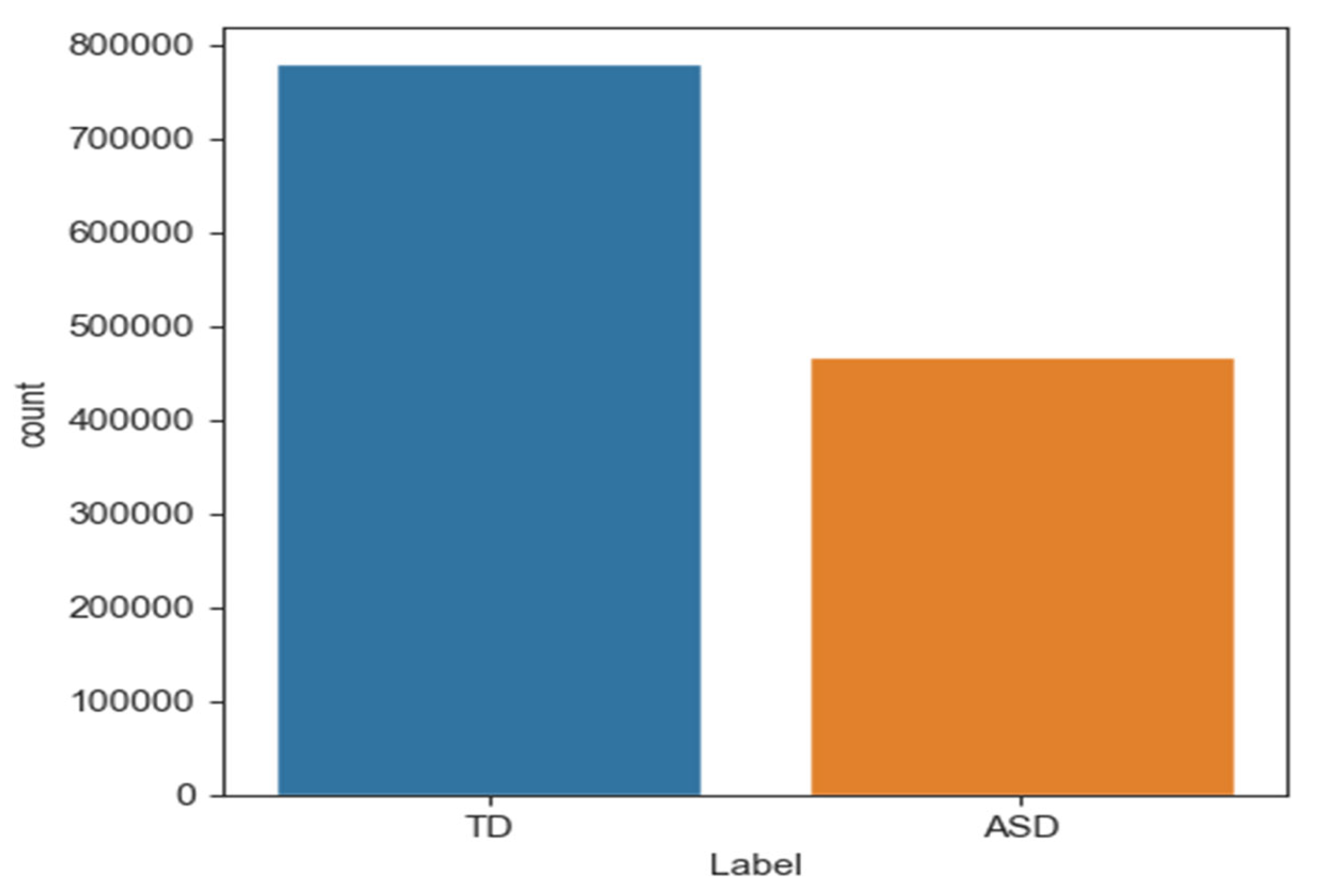
A fundamental aspect of the contributions presented in this study encompasses the deep learning-based model meticulously designed to discern autism through analysing gaze patterns. This study is one of the first studies to use the dataset after it was released as a standard dataset available to the public. The dataset comprises raw eye-tracking data collected from 29 children diagnosed with autism spectrum disorder (ASD) and 30 typically developing (TD) children. The visual stimuli used to engage the children during data collection included both static images (balloons and cartoon characters) and dynamic videos. In total, the dataset contains approximately 2,165,607 rows of eye-tracking data recorded while the children viewed the stimuli.

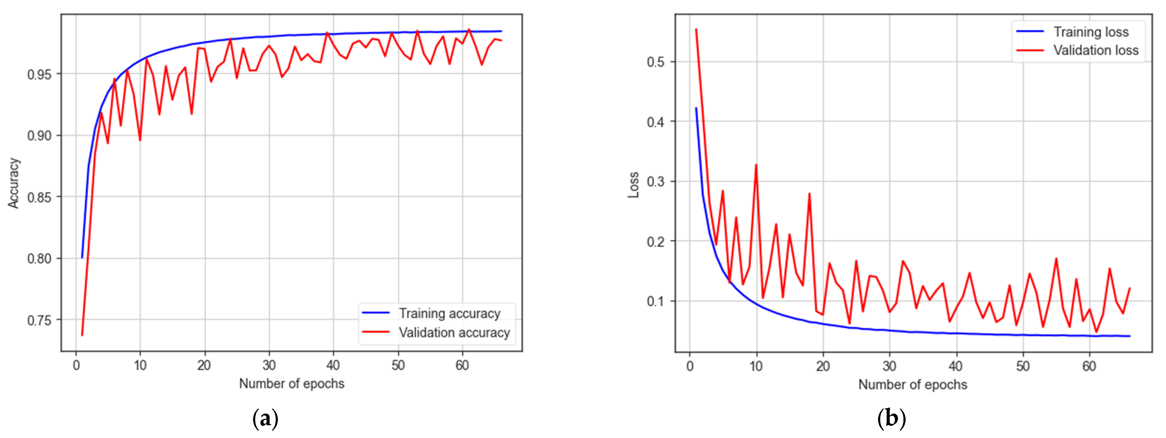
This study presented an impressive accuracy level of 98%, marking a notable stride in innovative advancement. This achievement is primarily attributed to the strategic implementation of the long short-term memory (LSTM) architecture, a sophisticated computational framework. The discernible success achieved substantiates the effectiveness of the rigorous preprocessing methodologies meticulously applied to the dataset, thereby underlining the robustness and integrity of the research outcomes.

This paper is organised as follows: section two discusses related work and previous studies that pertain to our research; section three presents the description of the data and the architecture of the models; section four provides the experimental results of the models and provides a detailed discussion. Finally, the conclusions of the study are presented.

2. Related Work

Neuroscience and psychology researchers employ eye-tracking equipment to learn crucial things about human behaviour and decision making. This equipment also aids in the identification and management of psychological problems like autism. For instance, people with autism may exhibit atypical gaze patterns and attention, such as a protracted focus on non-social things and issues synchronising their attention with social interactions. Eye-tracking technology can detect three main types of eye movements: fixation, saccade, and blinking. During fixation, the eyes briefly pause while the brain processes visual information. Fixation duration usually lasts between 150 ms and 300 ms, depending on the context. For instance, the duration differs when reading on paper (230 ms) compared to on a screen (553 ms) or when watching a naturalistic scene on a computer (330 ms) [6]. Saccades are rapid eye movements that continuously scan the object to ensure accurate perception, taking about (30–120 ms) each [7]. When the eye-tracking system fails to track gaze, a blink occurs.

This section provides a comprehensive review of previous study efforts that have utilised eye-tracking technology to examine disparities in gaze patterns and attentional mechanisms between individuals who have received a diagnosis of ASD and those who have not been diagnosed with ASD. This study focuses on the utilisation of artificial intelligence algorithms to diagnose autism through the analysis of gaze patterns. By combining eye-tracking technology with AI algorithms, this can help in the early detection of autism by analysing and classifying these gaze patterns (Ahmed and Jadhav, 2020; Kollias et al., 2021 [8,9]).

Eye-tracking technology has played a pivotal role in discerning the unique gaze and face recognition patterns exhibited by individuals with ASD. This subsection delves into how individuals with ASD and TD children differ in their visual attention toward faces. A study investigated whether children with ASD exhibit different face fixation patterns compared to TD children when viewing various types of faces, as proposed by (Kang et al., 2020a [10]). The study involved 77 children with low-functioning ASD and 80 TD children, all between the ages of (3 and 6) years. A Tobii TX300 eye-tracking system was used to collect data. The children sat 60 cm away from the screen and viewed a series of random facial photos, including own-race familiar faces, own-race unfamiliar faces, and other-race unfamiliar faces. The features were extracted using the K-means algorithm and selected based on minimal redundancy and maximal relevance. The SVM classifier was then used, with the highest accuracy of 72.50% achieved when selecting 32 features out of 64 from unfamiliar other-race faces. For own-race unfamiliar faces, the highest accuracy was 70.63% when selecting 18 features and 78.33% when selecting 48 features. The classification result AUC was 0.89 when selecting 120 features. The machine learning analysis indicated differences in the way children with ASD and TD processed own-race and other-race faces.

An approach to identify autism in children using their eye-movement patterns during face scanning was proposed by (Liu et al., 2016 [11]). A dataset was collected from 29 children with ASD and 29 TD children aged (4–11) years, using a Tobii T60 eye tracker with a sample rate of 60 Hz. During the stimuli procedure, the children were asked to memorise six faces and were then tested by showing them 18 faces and asking if they had seen that face before. The eye tracker recorded the children’s eye-scanning patterns on the faces. The K-means algorithm was used to cluster the eye-tracking data according to fixation coordinates. A histogram was then used to represent the features, and SVM was used for classification, resulting in an accuracy of 88.51%. The study found that eye-movement patterns during face scanning can be used to discriminate between children with ASD and TD children.

The study differentiation of ASD and TD was based on gaze fixation times as proposed by (Wan et al., 2019 [5]). The study included 37 participants with ASD and 37 TD individuals, all between the ages of (4 and 6) years. The researchers employed a portable eye-tracking system, specifically the SMI RED250 to collect data. The participants were placed in a dark, soundproof room and asked to view a 10 s silent video of a young Asian woman speaking the English alphabet on a 22-inch widescreen LCD display. The researchers used an SVM classifier, which yielded an accuracy of 85.1%. Analysis of the results revealed that the ASD group had significantly shorter fixation periods in various areas, including the eyes, mouth, nose, person, face, outer person, and body.

A validation of eye tracking as a tool for detecting autism was proposed by (Murias et al., 2018 [12]). Their study involved 25 children with ASD between the ages of (24 and 72) months, and eye tracking was conducted using a Tobii TX300 eye tracker. The Tobii TX300 Eye Tracker is a product of Tobii AB (Stockholm, Sweden) a Swedish technology company that develops and sells products for eye tracking and attention computing. The children were seated on their parent’s lap while watching a 3 min video of an actor speaking in a child-directed manner while four toys surrounded him. The researchers analysed the children’s eye gaze on the actor, toys, face, eyes, and mouth. The results suggest that eye-tracking social attention measurements are valid and comparable to caregiver-reported clinical indicators.

The gaze patterns of toddlers and preschoolers with and without ASD were compared as they watched static and dynamic visualisations as proposed by (Kong et al., 2022 [13]). The authors employed the SMI RED250 portable eye-tracking system to collect data from both ASD and TD children. The sample included 55 ASD and 40 TD toddlers aged between 1 and 3 years and 37 ASD and 41 TD preschoolers aged between 3 and 5 years. Participants were shown a video of a person moving his mouth while their eye movements were recorded. The study’s outcome indicated that the SVM achieved an 80% classification rate for both ASD and TD toddlers and 71% for preschoolers. The findings suggested that eye-tracking patterns for ASD in both toddlers and preschoolers were typical and distinctive.

The integration of eye-tracking technology with web browsing and searching provides a perceptive lens into people’s digital conduct, especially when comparing people with ASD and TD individuals. The investigation of eye-gaze patterns of TD and ASD individuals while browsing and searching web pages was introduced by (Yaneva et al., 2018 [14]). The study utilised several web pages like Yahoo, Babylon, Apple, AVG, Godaddy, and BBC. The participants included 18 TD and 18 ASD individuals under the age of 18 who were familiar with the web pages. The researchers employed the Gazepoint GP3 eye-tracking device to collect data on various gaze features, including time to first view, time viewed, fixations, and revisits. The collected data were then used to train a logistic regression model that included both gaze and non-gaze features. The results showed that the search task elicited more significant between-group differences, with a classifier trained on these data achieving 0.75 accuracy, compared to 0.71 for the browse task. The differences in eye tracking between web users with ASD and TD individuals were observed as proposed by (Eraslan et al., 2019 [15]). The participants’ eye movements were recorded while searching for specific information on various web pages. The study found that participants with ASD had longer scan paths and tended to focus on more irrelevant visual items and had shorter fixation durations compared to TD participants. The researchers also discovered different search patterns in participants with ASD. In a related study by (Deering 2013), eye-movement data were collected from four individuals with ASD and ten individuals without ASD while evaluating web content. The study examined eye fixation and movement patterns on various websites, including Amazon, Facebook, and Google. The findings indicated no significant differences between the two groups. However, (Eraslan et al., 2019 [15]) noted that the study’s sample size was limited.

The difference between ASD and TD groups was investigated in the reading task (Yaneva et al., 2016 [16]). The dataset was collected from 20 adults with ASD (mean age = 30.75) and 20 TD adults (mean age = 30.81) using the Gazepoint GP3 with a 60 Hz sampling rate. The study formulated several hypotheses, including the average number of fixations and longer fixations. The results showed that the ASD group had longer fixations on long words compared to the TD group. However, the study’s limitation was the eye tracker’s 60 Hz sampling rate, which may not be sufficient to accurately record the fixations while reading each word.

The study conducted by (Eraslan et al., 2021 [17]) aimed to evaluate the web accessibility rules related to the visual complexity of websites and the distinguishability of web page components, such as WCAG 2.1 Guideline 1.3 and Guideline 1.4. Gaze data were collected from two different types of information processing activities involving web pages: browsing and searching. Participants included 19 individuals with ASD with a mean age of 41.05 and 19 TD individuals with a mean age of 32.15. The Gazepoint GP3 eye tracker was used, and stimulating web pages such as BCC and Amazon were presented. The results revealed that the visual processing of the two groups differed for the synthesis and browsing tasks. The ASD group made considerably more fixations and transitions between items when completing synthesis tasks. However, when participants freely navigate the sites and concentrate on whatever aspects they find fascinating, the numbers of fixations and transitions are comparable across the two groups, but those with autism had longer fixations. The study found that there were significant differences between the two groups for the mean fixation time in browsing tasks and the total fixation count and number of transitions between items in synthesis tasks.

This subsection related to fixation time and visualising patterns within eye tracking delves into the specific metrics and patterns that characterise how eyes engage with visual stimuli. Carette et al. (2018 [18]) presented a method for transforming eye-tracking data into a visual pattern. They collected data from 59 participants, 30 TD and 29 ASD, using the SMI RED mobile eye tracker, which records eye movements at a 60 Hz frequency. Their dataset contains 547 images: 328 belonged to the TD class and 219 to the ASD class. They used these data to develop a binary classifier using a logistic regression model and achieved an AUC of approximately 81.9%. Subsequent work on this dataset employed deep learning and machine learning models, including random forests, SVM, logistic regression, and naive Bayes, with AUCs ranging from 0.7% to 92%. Unsupervised techniques such as deep autoencoders and K-means clustering were proposed by Elbattah et al. (2019 [19]), with clustering results ranging from 28% to 94%. A CNN-based model by Cilia et al. (2021 [20]) achieved an accuracy of 90%. Transfer learning models like VGG-16, ResNet, and DenseNet were evaluated, with VGG-16 having the highest AUC at 0.78% (Elbattah et al., 2022 [21]). The collective work underscores the growing interest and success in employing eye-tracking technology and various machine learning techniques to detect Autism, and highlights the need for improved sample sizes and dataset variations.

The eye movement was converted into text sequences using NLP as proposed by (Elbattah et al., 2020 [22]). To achieve this, the authors employed a deep learning model for processing sequence learning on raw eye-tracking data using various NLP techniques, including sequence extraction, sequence segmentation, tokenisation, and one-hot encoding. The authors utilised CNN and LSTM models. The LSTM model achieved 71% AUC, while the CNN achieved an AUC of 84%.

The Gaze–Wasserstein approach for autism detection is presented by (Cho et al., 2016 [23]). The data were collected using Tobii EyeX from 16 TD and 16 ASD children aged between 2 and 10 years. During the experiment, the children were seated in front of a screen and shown eight social and non-social stimuli scenes, each lasting for 5 s. The study utilised the KNN classifier and performance was measured using F score matrices. The overall classification scored 93.96%, with 91.74% for social stimuli scenes and 89.52% for non-social stimuli scenes. The results suggest that using social stimuli scenes in the Gaze–Wasserstein approach is more effective than non-social stimuli scenes.

The study employed machine learning to analyse EEG and eye-tracking (Kang et al., 2020b [24]) data from children, focusing on their reactions to facial photos of different races. Various features were analysed using a 128-channel system for EEG and the TX300 system for eye tracking. Feature selection was conducted using the minimum redundancy maximum relevance method. The SVM classifier achieved 68% accuracy in EEG analysis, identifying differences in power levels in children with autism spectrum disorder (ASD) compared to typically developing children. Eye-tracking analysis achieved up to 75.89% accuracy and revealed that children with ASD focused more on hair and clothing rather than facial features when looking at faces of their own race.

In recent years, there have been substantial advancement researches for classification and identifying ASD using different machine leaning algorithms based on the features of ASD people like face and eye tracking [25,26,27,28,29]. Thabtah et al. [30] proposed a study that collected a dataset from ASD newborns, children, and adults. The ASD was developed based on the Q-CHAT and AQ-10 assessment instruments. Omar et al. [31] used the methodology based on random forest (RF), regression tree (CART), and random forest iterative for detecting the ASD. The system used AQ-10 and 250 real-world datasets using the ID3 algorithm. Sharma et al. [32] proposed NB, stochastic gradient descent (SGD), KNN, RT, and K-star, in conjunction with the CFS-greedy stepwise feature selector.

Satu et al. [33] used a number of methods to detect ASD in order to determine the distinguishing features that differentiate between autism and normal development with different ages from 16 to 30 years. Erkan et al. [34] used the KNN, SVM, and RF algorithms to assess the efficacy of each technique in diagnosing autism spectrum disorders (ASDs). Akter et al. [35] used the SVM algorithm to demonstrate the superior performance of both toddlers and older children and adult datasets.

Despite the advancements in the amalgamation of eye-tracking methodologies with artificial intelligence techniques, a discernible research lacuna persists. This underscores the necessity for developing a model with superior performance capabilities to enhance classification precision, thereby ensuring a reliable early diagnosis of autism.

Table 1. Important existing studies.

Authors	Participations	Type of Study/Stimuli	Preprocessing	Method	Results and Founding
Wan et al., 2019 [5]	37 ASD and 37 TD at age (4–6) years	10 s silent video of a young Asian woman speaking the English alphabet		SVM	The SVM model achieved 85.1% accuracy
Elbattah et al., 2020 [22]	30 TD and 29 ASD at age (≈3—13) years		NLP techniques extraction of sequences, segmentation of sequences, tokenisation, and one-hot encoding	CNN and LSTM	CNN 84% AUC and LSTM 71% AUC
Kang et al., 2020 [10]	77 children with low-functioning ASD and 80 TD at age (3–6) years	Watched a series of random facial photos, such as photos of other-racial faces, own-racial unfamiliar faces, and own-racial familiar faces	The k-means algorithm is used to extract the features	SVM	The classification result AUC was 89% by selecting 120 features
Kong et al., 2022 [13]	55 toddlers with ASD and 40 TD children at age (1–3) years. Preschool children with 37 ASD and 41 TD at age (3–5) years.	Watched static and dynamic visualisation		SVM	The classification result of toddlers with ASD and TD SVM achieved 80%, while the preschoolers with ASD and TD SVM achieved 71%
Kang et al., 2020 [24]	9 ASD and 48 TD at age (3–6) years	The children watched a sequence of facial photos arranged at random	The features for EGG were the relative power of delta, theta, alpha, beta, and gamma. The features of eye tracking, such as body, background, face, eyes, right eye, left eye, and nose, are the eight AOIs used for facial image analysis.	SVM	The EGG result is 68% accurate, while the accuracy of eye tracking is 75.89%
Yaneva et al., 2018 [14]	15 TD and 15 ASD under the age of 18 years	Eye gaze during the browsing and searching of web pages	Gaze features and non-gaze features	Logistic regression	The model trained on these data achieved 75% accuracy results compared to 71 for the browse task
Liu et al., 2016 [11]	29 ASD and 29 TD at age (4–11) years	Asking the children to memorise six faces, then testing them by showing 18 faces and asking them if they saw that face or not during that time	The K-means algorithm has been used to cluster the eye tracking according to fixation coordinates then the feature is represented as a histogram	K-means SVM	SVM was used for classification which achieved 88.51% accuracy

displays the most important previous studies.

3. Materials and Methods

This study proposed a methodology for autism identification utilising deep learning models applied to the eye-tracking dataset. It aims to enhance the efficiency and accuracy of autism detection. This methodology follows several steps such as data preparation, data cleaning and features selection, and data balancing to improve the model performance. Thereafter, deep learning models, such as LSTM, CNN-LSTM, Bi-LSTM, and GRU, have been applied. Figure 1 shows the proposed methodology.

3.1. Dataset

In this study, a publicly available dataset named “Eye-Tracking Dataset to Support the Research on Autism Spectrum Disorder” [36] has been used. It comprises a raw statistical dataset of the eye-tracking dataset. The dataset was collected from 29 ASD and 30 TD children, as shown in

Table 2. Details of participant datasets [25].

Details		ASD Group	TD Group
Gender	Female	4	17
	Male	25	13
Total		29	30
Age Mean		µ = 7.88

.

The dataset developers used an RED mobile eye tracker with a sampling rate of 60 Hz for data collection. The eye tracker was connected to A 17-inch screen for a stimulating display. The dataset developers [36] have followed some procedures, such as the special place for the experiment. The participants sat 60 cm away from the screen to allow the eye tracker to track their eye movements by reflecting infrared lights. For this investigation, the visual stimuli including static and dynamic have been used. The dynamic stimuli included video scenarios that incorporated a specific design to engage children, including balloons and cartoon characters. The static stimulation comprises various visual elements such as facial images, objects, cartoons, and other stimuli specifically intended to evoke a sense of grabbing the participants’ attention. The experiment had a length of around five minutes, during which the arrangement of items was subject to variation. The stimuli employed in the study comprised movies with a human presenter delivering a speech. The primary objective of these videos was to engage the participants’ attention toward different elements displayed on the screen, regardless of their visibility. Through these videos, information regarding eye contact, engagement level, and gaze focus can be obtained. This dataset was used to investigate the differences in visual patterns of ASD and TD children, such as fixations, saccades, and blink rate, to understand the subject’s visual attention [36]. After recording all sessions, the dataset comprises approximately 2,165,607 rows. The dataset was gathered from individuals both diagnosed with ASD and those with TD.

Table 3. Summary of essential dataset features.

Parameter (Feature Name)	Features Description
Recording Time [ms]	Time stamp of the sample in (microseconds)
Trial	Number of current trials
Stimulus	Stimulus name
Participant	Subject code
Tracking Ratio [%]	Is a measure of the accuracy of an eye-tracking system. It is calculated as the percentage of samples where the eye-tracking system accurately tracks the eye’s position
Category Group	Information/eye
Category Right/Left	Separator/fixation/saccade/blink
Pupil Size Right/Left X [px]	Horizontal pupil size in pixels
Pupil Size Right/Left Y [px]	Vertical pupil size in pixels
Pupil Diameter Right/Left [mm]	Circular pupil diameter in mm
Point of Regard Right/Left X [px]	Horizontal point of regard
Point of Regard Right/Left Y [px]	Vertical point of regard
AOI group Right/Left	AOI group right/left
AOI Scope Right/Left	Rightmost/leftmost edge of an area of interest
AOI Order Right/Left	Could refer to a sequence or ranking of AOIs
AOI Name Right/Left	Refers to a specific region or location on the right/left side of a computer screen
Gaze Vector on Right/Left X	Refers to the X direction in which a person is looking with their right/left eye
Gaze Vector on Right/Left Y	Refers to the Y direction in which a person is looking with their right/left eye
Gaze vector on Right/Left Z	Depth direction of gaze
Eye Position X [mm]	Horizontal position of the eye, measured in millimetres
Eye Position Y [mm]	Vertical position of the eye, measured in millimetres
Eye Position Z [mm]	Distance of the eye from a reference point
Pupil Position Right/Left X [px]	Refers to the horizontal position of the pupil in pixels in a two-dimensional image or video frame captured by an eye-tracking device
Pupil Position Right/Left Y [px]	Refers to the vertical position of the pupil in pixels in a two-dimensional image or video frame captured by an eye-tracking device

provides an explanation of the features within the statistical dataset.

3.2. Data Preprocessing

The data preparation stage is a crucial component of the data analysis process, encompassing organising, cleaning, and transforming raw data to guarantee its accuracy and dependability (Dasu and Johnson, 2003 [37]). The primary objective of this stage is to appropriately preprocess the data to facilitate subsequent modelling and analytical tasks. This involves the feature selection of relevant characteristics, addressing any missing or erroneous values and appropriately scaling the data.

3.2.1. Data Labelling

This research employed an unlabelled dataset of around 2,165,607 samples, presented in 25 CSV files. We allocated labels to the dataset according to the participant identification number to facilitate the utilisation of supervised learning techniques. Labelling was conducted using the data provided in the associated dataset information. The act of labelling plays a vital role in supervised learning as it furnishes the model with both the input data and related targets, thereby enabling the precise prediction of outputs.

3.2.2. Data Encoding

In the eye-tracking dataset, it is necessary to transform specific categorical attributes into numerical representations to enable efficient processing by a deep learning algorithm. To achieve this objective, the methodology of label encoding was utilised. The process of label encoding involves converting categorical data into numerical data by assigning a separate number value to each unique category inside the variable. The dataset has several categorical features such as “Trial”, “Stimulus”, “Color”, “Category Right”, and “Category Left”.

3.2.3. Missing Values Processing

The missing values in eye-tracking data can arise due to various factors. These factors may include technical issues in the eye-tracking equipment, participants’ lack of focus or physical movements, or data loss during the recording phase. The appropriate management of missing values is crucial to ensure the integrity and validity of the results obtained from the model. Several approaches address missing values such as deleting the missing data, imputing missing values, performing multiple imputations, and utilising a portion of the available data.

The “ffill” approach from the panda’s library was employed in this study to address the issue of missing values in the eye-tracking dataset. The choice is based on the systematic approach used in obtaining eye-tracking data. The “ffill” method utilises this characteristic by replacing missing values with the most recent non-missing value discovered in the associated column. Implementing this methodology guaranteed the reliability and accuracy of the data analysis procedure (McKinney, 2012 [38]).

3.2.4. Features Selection

This research paper concerns the feature selection procedure associated with analysing eye-tracking data to discover patterns that may be symptomatic of ASD. Choosing pertinent features from the vast volume of data produced by eye-tracking experiments is crucial in ensuring the efficacy of deep learning models. Our research aims to examine the potential enhancement of deep learning models through the utilisation of feature selection approaches. Through feature reduction and model interpretability enhancement, it becomes possible to discern patterns within eye-tracking data that serve as indicators for ASD.

Feature selection was conducted on the dataset to determine the most crucial and pertinent aspects to identify Autism. The process entailed analysing the information to identify common traits across all files that were considered indicative of autism. The dataset’s dimensionality was considered, with certain files containing 26 features and others containing more than 50. Additionally, it was observed that certain features within the dataset were either empty or exhibited strange characteristics. Our objective was to carefully choose the most pertinent and useful elements to detect autism effectively. Several features were considered from the dataset, including fixation (1,365,901 occurrences), blink (347,390 occurrences), saccade (182,401 occurrences), “-“ (128,343 occurrences), separator (5340 occurrences), and left click (1 occurrence). Our analysis focuses on the features of fixation, blink, and saccade. In addition, we prioritise the eye category inside the category group feature, specifically eye 202,4035 and information 5341. After completing all the necessary preprocessing steps, including data cleaning and feature selection, our dataset comprised 1,166,211 records and 16 features.

The random forest method was used to evaluate features and their impact on models trained on eye-tracking data to identify ASD patterns. This method estimates the average decrease in impurity or increase in information gain from splitting the dataset on each feature to determine its importance in training the model. The average decrease in impurity or increase in information gain across all random forest decision trees determines feature importance. A higher feature importance value means the feature is better at predicting and distinguishing classes. Figure 2 shows the importance of feature scores.

3.2.5. Data

The input data feature distribution is the frequency or pattern of different values or value ranges within each feature. It shows how feature values are distributed across the entire range. Figure 3 shows a graphical representation of this distribution. Understanding the feature distribution in input data can help with feature selection, scaling, and model selection in many machine learning tasks. Visualising feature distributions can also reveal data outliers that may need to be addressed before modelling.

The relationship between two variables can be measured using a correlation coefficient. A heatmap is a valuable graphical depiction of the correlation coefficients between two attributes within a dataset, rendering it a beneficial instrument for data analysis. The heatmap effectively demonstrates the characteristics and orientations of the linkages among nodes by employing a colour scheme. The heatmap depicted in Figure 4 illustrates the presence of positive correlations through the use of darker colours, while brighter colours visually represent negative correlations. This colour scheme enhances the visibility of a comprehensive entity’s interrelated constituents. Utilising a heatmap facilitates the acquisition of significant insights from a dataset by visually emphasising the interconnections among different attributes.

3.2.6. Data Scaling

Machine learning and statistics use the standard scaler to standardize dataset features. Standardising a dataset involves adjusting feature values to a mean of 0 and a standard deviation of 1 [39]. This ensures that all features are standardised to a common scale, preventing any one feature from dominating the model fitting process.

3.2.7. Data Splitting

Data splitting divides the dataset into subsets for effective training, validation, and testing of machine learning models. A dataset is split into three subsets: training, validation, and test sets. This partitioning aids in model training, validation, and evaluation of generalisation to unseen data. This practice ensures accurate assessment and reduces overfitting by preventing the model from over-optimising performance metrics.

3.2.8. Data Imbalanced Processing

Data imbalance occurs when one category or class is overrepresented in machine learning models. The model may predict the dominant class well, but poorly predict the underrepresented class. Thus, biased or unjust predictions can lead to negative outcomes, especially when the minority class is marginalised. Oversampling techniques have been proposed to address data imbalance. This study addressed imbalanced datasets with SMOTE [40]. Figure 5 shows that “ASD” had 416,682 samples and “TD” had 749,529 samples. After dividing the data into training and testing sets, 599,623 samples were typically developing (TD) and 333,345 were ASD. SMOTE was applied only to training data to address this issue.

Table 4. Data balancing.

Class Name	Training Dataset before SMOTE	Training Dataset after SMOTE
ASD	333,345	599,623
TD	599,623	599,623

shows that this method produced a balanced dataset with 599,623 samples for each class.

3.3. Deep Learning

Deep learning involves focusing on a premium using large datasets for training neural networks to learn and make predictions. The network’s design aims to develop an environment that is functionally analogous to the human brain [41]. The use of deep learning has been applied in many fields, such as computer vision, NLP, speech recognition, data science, and even autonomous vehicles. This method is helpful because it can automatically extract meaningful features from raw data without requiring human-designed add-ons, and thus saves time and effort.

3.3.1. Recurrent Neural Networks

Recurrent neural networks (RNNs) are a type of neural network specifically developed to process sequential data effectively [42]. In contrast to conventional feedforward networks, RNNs have loops that facilitate the retention of information, and thus permit the preservation of a memory of preceding inputs. The presence of internal memory in RNNs enables them to capture temporal relationships and patterns in sequences effectively. As a result, RNNs are highly suitable for many tasks, including time series prediction, natural language processing, and any application where preserving data order and continuity is crucial. Nevertheless, it is worth noting that basic RNNs sometimes encounter difficulties in capturing long-term dependencies, mostly due to the vanishing gradient problem. As a result, more advanced variants such as long short-term memory (LSTM) and gated recurrent units (GRUs) have been developed to tackle this challenge specifically.

3.3.2. Deep Learning Models

In particular, CNNs and RNNs are appropriate for analysing eye-tracking data, which comprise numerical coordinates reflecting the positions of gaze over time. Most researchers associate CNNs primarily with conducting image processing operations. One-dimensional data, such as eye-tracking sequences, can also associate CNNs with gaze patterns. RNNs have the ability to handle sequential input, which improves this capacity by displaying great competence in understanding the temporal dependencies among these features. RNNs can capture the dynamic development of eye movements by keeping track of previous time steps in a series. As a result, they can shed light on the mental operations or behavioural patterns that underlie eye-tracking data. Combining CNNs for spatial pattern recognition with RNNs for temporal analysis provides a solid basis for making sense of eye-tracking data. Several disciplines, such as user experience design, psychological research, and medical diagnosis, could benefit from incorporating this collaborative approach.

3.3.3. Long Short-Term Memory Model

Long short-term memory (LSTM) is a special kind of RNN architecture developed to address the issue of decreasing gradients that can occur during the training of regular RNNs when applied to tasks with long-term dependencies (Hochreiter & Schmidhuber, 1997 [43]). The LSTM model incorporates memory cells, hidden states, and gating mechanisms to deal with this problem.

The LSTM model comprises LSTM cells, which comprise three gates: an input gate, a forget gate, and an output gate. The functioning of these gates is facilitated by the utilisation of sigmoid activation functions, which effectively control the influx and efflux of information within the cell. The input gate governs the ingress of new data into the cell, the forget gate manages the selective removal of information from the internal state of the cell, and the output gate regulates the passage of data from the cell to the output. The mathematical formulation for LSTM is represented by the following equations:

The input gate:

$$i\_t=\sigma \left(W\_ix\_t+U\_ih\_\left\{t-1\right\}+b\_i\right)$$

(1)

The forget gate:

$$f\_t=\sigma \left(W\_fx\_t+U\_fh\_\left\{t-1\right\}+b\_f\right)$$

(2)

The memory cell:

$$c_t=f_t\times c_{\left\{t-1\right\}}+i_t\times tanh\left(W_{c{x}_t}+U_{c{h}_{\left\{t-1\right\}}}+b_c\right)$$

(3)

The output gate:

$$o\_t=\sigma (W\_ox\_t+U\_oh\_\left\{t-1\right\}+b\_o$$

(4)

The hidden state:

$$h\_t=o\_t\times tanh\left(c\_t\right)$$

(5)

where x_t represents the input at time t, h_t represents the hidden state at time t, c_t represents the memory cell state at time t, i_t, f_t, o_t represent the input, forget, and output gates, respectively, and W, U, b represent the weights and biases of the network. The sigma function represents the sigmoid activation function, and tanh represents the hyperbolic tangent activation function.

The eye-tracking data analysis model utilising the LSTM model for autism detection includes an input layer comprising 1024 neurons, followed by a hidden layer comprising 512 neurons. This hidden layer is then linked to a fully connected layer containing 34 neurons, and the output from this layer is employed to forecast whether the subject has ASD or TD, as depicted in Figure 6. The LSTM architecture is intended to manage long-term dependencies in sequential data, which makes it suitable for eye-tracking data analysis in autism detection tasks. The interplay between the input and hidden layers and the use of gates in the LSTM cells enables intricate analysis of the input data and effective feature extraction for prediction purposes.

3.3.4. CNN-LSTM Model

The CNN-LSTM model provides a way to analyse eye-tracking data by combining the spatial understanding of CNNs with the temporal sequencing capabilities of LSTMs. Researchers and practitioners can gain valuable insights into human attention, cognition, and behaviour by carefully designing and training these networks.

The CNN-LSTM model comprises various layers with specific parameters. The first layer is a Conv1D layer with 16 filters and a kernel size of 2, trailed by a batch normalisation layer. Subsequently, another Conv1D layer exists with 32 filters and a kernel size of 2, which is again trailed by another batch normalisation layer. Once the convolutional layers are complete, the model encompasses an LSTM layer with 1024 units. This is followed by a dense layer containing 512 units, and another dense layer comprising 32 units. The model’s output is employed to anticipate whether the subject has ASD or TD, as demonstrated in Figure 7.

3.3.5. Gated Recurrent Units Model

Gated recurrent units (GRUs) are a kind of recurrent neural network design that emerged in 2014 as a substitute for LSTM units (Chung et al., 2014 [44]). GRUs aim to address the issue of vanishing and exploding gradients, which can make it challenging to train deep networks using traditional RNNs. GRUs employ gates, similar to LSTMs, to regulate the flow of information throughout the network. The GRU architecture comprises two crucial gates: the update and reset gates. The update gate controls the utilisation of the previous hidden state in the current hidden state, while the reset gate determines the extent to which the previous hidden state should be forgotten. Here are the equations that describe a GRU:

Update gate:

$$\mathrm{Reset} \mathrm{Gate}: zt=\sigma \left(Wz\cdot \left[ht-1,xt\right]+bz\right)$$

(6)

$$\mathrm{Candidate} \mathrm{Activation} rt=\sigma \left(Wr\times \left[ht-1,xt\right]+br\right)$$

(7)

$$\mathrm{Final} \mathrm{Activation}: h~t=tanh\left(W\times \left[rt\odot ht-1,xt\right]+b\right)$$

(8)

$$ht=\left(1-zt\right)\odot ht-1+zt\odot h~t$$

(9)

where xt is the input at time tt, ht − 1 is the hidden state from the previous time step, σ denotes the sigmoid function, ⊙ denotes element-wise multiplication, Wz, Wr, WWz, Wr, W are weight matrices for the update gate, reset gate, and candidate activation, respectively, and bz, br, bbz, br, b are the biases for the update gate, reset gate, and candidate activation, respectively.

These gates play a pivotal role in regulating the flow of information within the GRU network. Our research utilises GRUs to identify autism via eye-tracking data. The GRUs network is trained on eye-tracking data to detect Autism. The GRUs neural network comprises a GRU layer containing 1024 units, followed by a GRU layer comprising 512 units, and a dense layer containing 34 units. Eventually, the model delivers a binary classification, signifying whether the subject has ASD or TD. The model architecture is shown in Figure 8.

3.3.6. Bidirectional Long Short-Term Memory Model

Bidirectional long short-term memory (BiLSTM) is a proposed extension of the LSTM network design (Zhou et al., 2016 [45]). It is possible to handle sequential input in either direction with this deep learning network. This allows the network to make predictions about the future of the input sequence based on the information it has about the present. The BiLSTM can be used for non-linguistic processing, speech recognition, and time-series prediction. To process the input sequence of both forward and backward states, BiLSTM employs two LSTM architectures. The aggregate output of the networks is utilised to generate the final prediction’s features, which are then sent via a fully connected layer. This technique enables the network to comprehensively analyse the input data by capturing relationships between the past and future states of the input sequence. Here is a general idea of how it works:

Forward Pass (ht→):

$$ht=\mathrm{RNN}forward\left(xt,ht-1\right)$$

(10)

Backward Pass (ht←):

$$ht=\mathrm{RNN}backward\left(xt,ht+1\right)$$

(11)

For the final representation at time tt, you would typically concatenate the forward and backward hidden states:

$$ht=\left[\mathrm{ht}forward;\mathrm{ht}backward\right]$$

(12)

Our research utilises BiLSTM to identify autism via eye-tracking data. The BiLSTM network is trained on eye-tracking data to detect autism. The BiLSTM neural network comprises a bidirectional layer containing 128 LSTM units, followed by an LSTM layer comprising 32 units. Eventually, the model delivers a binary classification, signifying whether the subject has ASD or TD. The model architecture is shown in Figure 9.

4. Experimental Results

This section outlines our study’s experimental setup, evaluation metrics, and model performance.

4.1. Environment Setup

Our study’s experimental results were conducted on a laptop with hardware specifications including an 8th generation Intel Core i7 processor, 16 GB of RAM, and an NVIDIA GeForce GTX GPU with 8 GB. On the other hand, we utilised the TensorFlow framework [46] to develop our models. These requirements are used to train and evaluate our deep learning models effectively.

4.2. Evaluation Metrics

Assessing the effectiveness of deep learning models holds significance in comprehending their efficiency [47]. Various metrics come into play for this purpose, encompassing accuracy, sensitivity, precision, recall, F1 score, ROC curve, and confusion matrix. These evaluative metrics offer distinct perspectives on the model’s strengths and limitations.

4.3. Confusion Matrix

The assessment of binary classification models hinges on the utilisation of a confusion matrix, which outlines the predictive performance of the model on the test dataset. This matrix encompasses four distinct categories: True positives (TP) denote instances where the model accurately predicts ASD cases. False positives (FP) occur when the model incorrectly identifies negative cases (ASD) as positive (TD). True negatives (TN) represent the instances where the model correctly anticipates negative cases. Finally, false negatives (FN) indicate positive cases (TD) that the model erroneously classifies as negative (ASD).

4.4. Accuracy

The accuracy metric stands as a prevalent means for appraising the effectiveness of deep learning models. This metric measures the model’s predictive performance by determining the ratio of accurate predictions to the overall predictions made, as expressed in formula (12).

$$Accuracy=\frac{TP+TN}{TP+TN+FP+FN}\times 100$$

(13)

4.4.1. F1 Score

The F1 score represents the harmonic average of the recall and precision metrics. When evaluating the model’s effectiveness, precision and recall are considered. A high F1 score for the model indicates a well-balanced trade-off between precision and recall, which translates to an elevated accuracy by minimising false positive and negative predictions. The computation of the F1 score involves employing formula (13).

$$F1-score=2\times \frac{precision\times \mathrm{Recall} }{precision+ \mathrm{Recall} }\times 100$$

(14)

4.4.2. Sensitivity

Sensitivity relates to the true positive rate, signifying the proportion of accurately detected positive instances by a binary classification model in relation to the total actual positive instances. The computation of sensitivity is conducted using formula (14).

$$Sensitivity = \frac{True Positives }{True Positives+False positives }$$

(15)

In our investigation, sensitivity quantifies the model’s proficiency in accurately recognising true positive instances (ASD cases).

4.4.3. Specificity

The idea of specificity revolves around a binary classification model’s capability to precisely detect negative instances. It represents the proportion of correctly identified negative instances compared to the total number of negative instances predicted by the model. In simpler terms, this metric assesses the model’s effectiveness in avoiding false positives, which are cases that are genuinely negative but are inaccurately labelled as positive. The mathematical representation for specificity is as follows:

$$specificity=\frac{True Negatives}{True Negatives+False Negatives}$$

(16)

Specificity quantifies a model’s aptitude for accurately identifying negative instances (TD cases).

4.4.4. Receiver Operating Characteristic

The receiver operating characteristic (ROC) curve illustrates a binary classification model’s performance by plotting the true positive rate (TPR) against the false positive rate (FPR). The false positive rate (FPR) characterises the model’s instances of misclassifying negative examples. Conversely, the true positive rate (TPR) signifies the model’s accuracy in identifying positive examples. Through the ROC curve, the trade-off between true positives and false positives in the model becomes apparent, as it displays the relationship between TPR and FPR.

4.5. Results

4.5.1. Deep Learning Classification Results

This section provides the evaluation of the results produced from the deep learning models used in the statistical eye-tracking dataset-based experimental study aiming at detecting autism. LSTM, CNN-LSTM, GRU, and BiLSTM are all used as experimental models in this investigation.

4.5.2. BiLSTM Model Result

This study utilised the BiLSTM model with the parameters described in

Table 5. Parameters of the BiLSTM model.

Parameters	Values
LSTM units	64-unit first bidirectional LSTM layer
LSTM units	32-unit bidirectional LSTM layer
Activation function	Sigmoid
Optimiser	RMSprop with learning rate: 0.001
Callbacks	Early stopping with patience = 5
Epochs	200
Batch size	1024
Validation split	0.1

to detect autism using a statistical eye-tracking dataset.

The confusion matrix for ASD classification using the BiLSTM model, as shown in Figure 10, reveals 80,642 true positives, 2695 false positives, 5610 false negatives, and 144,296 true negatives.

The BiLSTM model was trained for 200 epochs and achieved a training accuracy of 97.72% and a testing accuracy of 96.44%, as shown in Figure 11. The model showcased a sensitivity of 93.50% and a specificity of 98.17%. Additionally, with an F1 score of 97.20%, the model achieved an AUC of 97%.

4.5.3. GRU Model Result

This study utilised the GRU model with the parameters described in

Table 6. Parameters of the GRU model.

Parameters	Details
GRU	1024 units
GRU	512 units
Dense	34 units
Activation Function	Sigmoid
Optimizer	RMSprop with learning rate: 0.001
Callbacks	Early stopping, model checkpoint
Epochs	200
Batch Size	1024
Validation Split	0.1

to detect autism using a statistical eye-tracking dataset.

The confusion matrix for ASD classification using the GRU model, as shown in Figure 12, reveals 80,959 true positives, 2378 false positives, 3473 false negatives, and 146,433 true negatives.

The GRU model was trained for 200 epochs with early stopping at 65 epochs. It achieves a training accuracy of 98.02% and a testing accuracy of 97.49%, as shown in Figure 13. The model demonstrates a sensitivity of 95.89%, a specificity of 98.40, and an F1 score of 98.04%. Additionally, the model achieves an AUC of 97%.

4.5.4. CNN-LSTM Model Result

This study utilised the CNN-LSTM model with the parameters described in

Table 7. Parameters of the CNN-LSTM model.

Parameters	Details
Conv1D	Filters: 16, kernel Size: 2, activation: relu, batch normalisation
Conv1D	Filters: 32, kernel Size: 2, activation: relu, batch normalisation
LSTM	1024 units
Recurrent Dropout	0.1
Dense	512 units
Dense	32 units
Activation Function	Sigmoid
Optimizer	RMSprop with learning rate: 0.001
Callbacks	Early stopping with patience = 5
Training	Epochs: 200
Batch Size	1024
Validation Split	0.1

to detect autism using a statistical eye-tracking dataset.

The confusion matrix for ASD classification using the CNN-LSTM model, as shown in Figure 14, reveals 81,537 true positives, 1800 false positives, 3008 false negatives, and 146,898 true negatives.

The CNN-LSTM model was trained for 200 epochs, and early stopping took place at 66 epochs. It attains a training accuracy of 98.41% and a testing accuracy of 97.94%, as shown in Figure 15. The model showcases a sensitivity of 96.44% and a specificity of 98.79%. With an F1 score of 98.70%, the model proves its effectiveness in autism detection. Additionally, the model achieves an AUC of 98%.

4.5.5. LSTM Model Result

This study utilised the LSTM model with the parameters described in

Table 8. Parameters of the LSTM model.

Parameters	Details
LSTM	1024, 512 units
Dense	34 units
Activation Function	Sigmoid
Optimizer	RMSprop with learning rate: 0.001
Callbacks	Early stopping with patience = 5
Epochs	200
Batch Size	1024
Validation Split	0.1

to detect autism using a statistical eye-tracking dataset.

The confusion matrix for ASD classification using the LSTM model, as shown in Figure 16, reveals 81,760 true positives, 1577 false positives, 2315 false negatives, and 147,591 true negatives.

The LSTM model underwent training for 200 epochs, and early stopping occurred at 141 epochs. It achieves a training accuracy of 98.99% and a testing accuracy of 98.33%, as indicated in Figure 17. The model demonstrates a sensitivity of 97.25% and a specificity of 98.94%. With an F1 score of 98.70%, the model proves its effectiveness in autism detection. Additionally, the model achieves an AUC of 98%.

5. Discussion

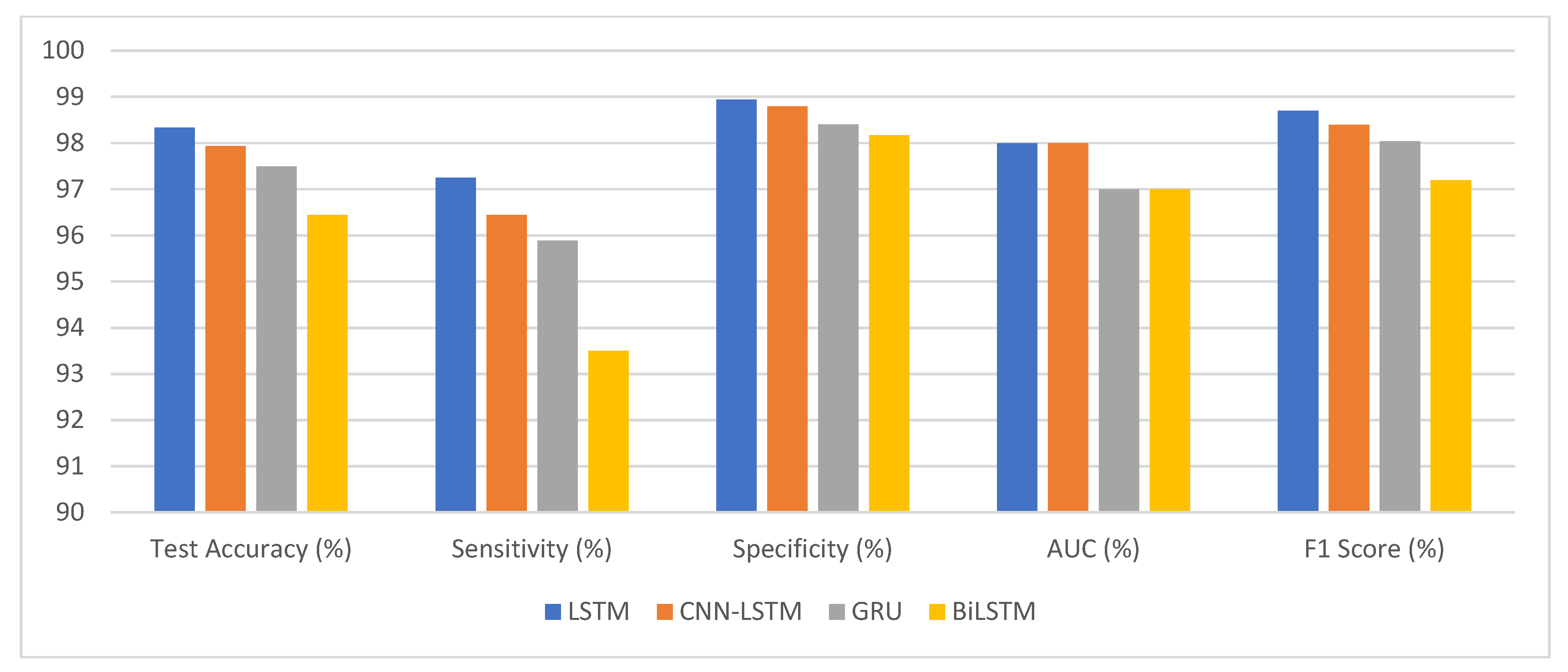
This research paper aims to enhance the diagnostic process of the ASD by combining eye-tracking data with deep learning algorithms. It investigates different eye-movement patterns in individuals with ASD compared to TD individuals. This approach can enhance ASD diagnosis accuracy and pave the way for early intervention programs that benefit children with ASD. The experimental work investigated the effectiveness of deep learning models, specifically LSTM, CNN-LSTM, GRU, and BiLSTM, in detecting autism using a statistical eye-tracking dataset. The findings shed light on the performance of these models in accurately classifying individuals with autism. Among the models, the LSTM model achieved an impressive test accuracy of 98.33%. It successfully identified 81,760 true positive samples, while maintaining a low false positive rate of 1577, out of the 84,075 ASD samples. With a high sensitivity of 97.25%, the model demonstrated its ability to detect individuals with autism accurately. Moreover, it exhibited a specificity of 98.94%, effectively identifying non-autistic individuals. The F1 score of 98.70% further emphasises the model’s effectiveness in autism detection.

The deep learning models performed well on a statistical eye-tracking dataset for autism detection as presented in

Table 9. Summary of our deep learning classification results.

Model Name	Test Accuracy (%)	TP	FP	FN	TN	Sensitivity (%)	Specificity (%)	AUC (%)	F1 Score (%)
BiLSTM	96.44	80,642	2695	5610	144,296	93.50	98.17	97	97.20
GRU	97.49	80,959	2378	3473	146,433	95.89	98.40	97	98.04
CNN-LSTM	97.94	81,537	1800	3008	146,898	96.44	98.79	98	98.39
LSTM	98.33	81,760	1577	2315	147,591	97.25	98.94	98	98.70

and Figure 18. Accuracy rates, sensitivities, and specificities all point to their usefulness in identifying autistic people. These results proposed that deep learning models may be useful in autism diagnosis. They could help advance efforts towards better screening for autism and more timely treatments for those on the spectrum.

In the evolving domain of research aimed at distinguishing autism spectrum disorder (ASD) from typically developing (TD) individuals, various methodologies have emerged, offering rich insights. Liu et al. (2016), employing an SVM-based model focused on facial recognition, achieved an accuracy of 88.51%, hinting at significant neural disparities in processing between ASD and TD children. Similarly, Wan et al. (2019) leveraged visual stimuli, specifically videos, to attain an accuracy of 85.1% with SVM, emphasising the diagnostic potential of the visual modality. An intriguing age-centric variation was observed in Kong et al. (2022), where SVM-analysed toddlers and preschoolers demonstrated accuracies of 80% and 71%, respectively, underscoring the necessity for age-adaptive diagnostic strategies. Shifting focus, Yaneva et al. (2018) delved into eye-gaze pat terns, achieving results of 0.75 and 0.71 for search and browsing tasks through logistic regression, suggesting that gaze metrics could be pivotal in ASD diagnostics. Meanwhile, Elbattah et al., 2020 used CNN and LSTM models to analyse static and dynamic scenes, obtaining accuracies of 0.84% and 71%.

Upon a comprehensive examination and comparison of extant literature, it is evident that our proposed model exhibits marked efficacy and superiority as presented in

Table 10. Comparative analysis of our classification models with existing models.

Authors	Participations	Type of Study/Stimuli	Preprocessing	Method	Results
Liu et al. (2016) [11]	29 ASD and 29 TD children (4–11 years)	Memorisation and recognition of faces	K-means clustering, histogram representation	SVM	88.51%
Wan et al. (2019) [5]	37 ASD and 37 TD individuals (4–6 years)	Video of a woman speaking the English alphabet		SVM	85.1%
Kong et al. (2022) [13]	55 ASD and 40 TD toddlers (1–3 years), 37 ASD and 41 TD preschoolers (3–5 years)	Video of a person moving their mouth		SVM	80% classification rate for toddlers, 71% for preschoolers
Yaneva et al. (2018) [14]	18 TD and 18 ASD individuals (<18 years)	Eye-gaze patterns while browsing and searching web pages (e.g., Yahoo and Apple)	Gaze features: time to first view, time viewed, fixations, revisits	Logistic regression (gaze and non-gaze features)	Search task classifier: 75% accuracy. Browse task classifier: 71% accuracy.
Elbattah et al., 2022 [22]	30 TD and 29 ASD at age (≈3–13) years	Static and dynamic natural scenes	NLP techniques extraction of sequences, segmentation of sequences, tokenisation, and one-hot encoding	CNN and LSTM	CNN 84% AUC and LSTM 71% AUC
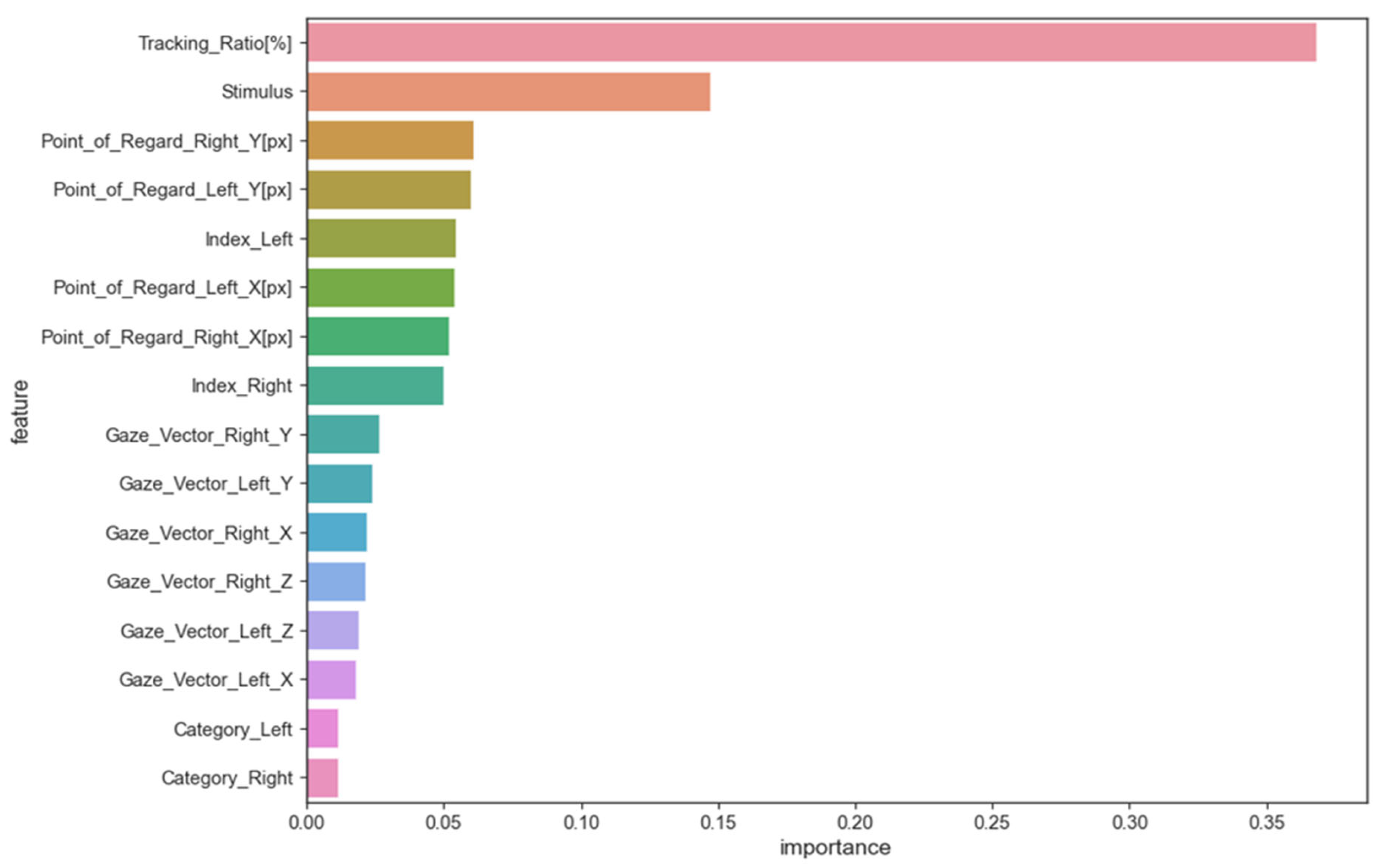
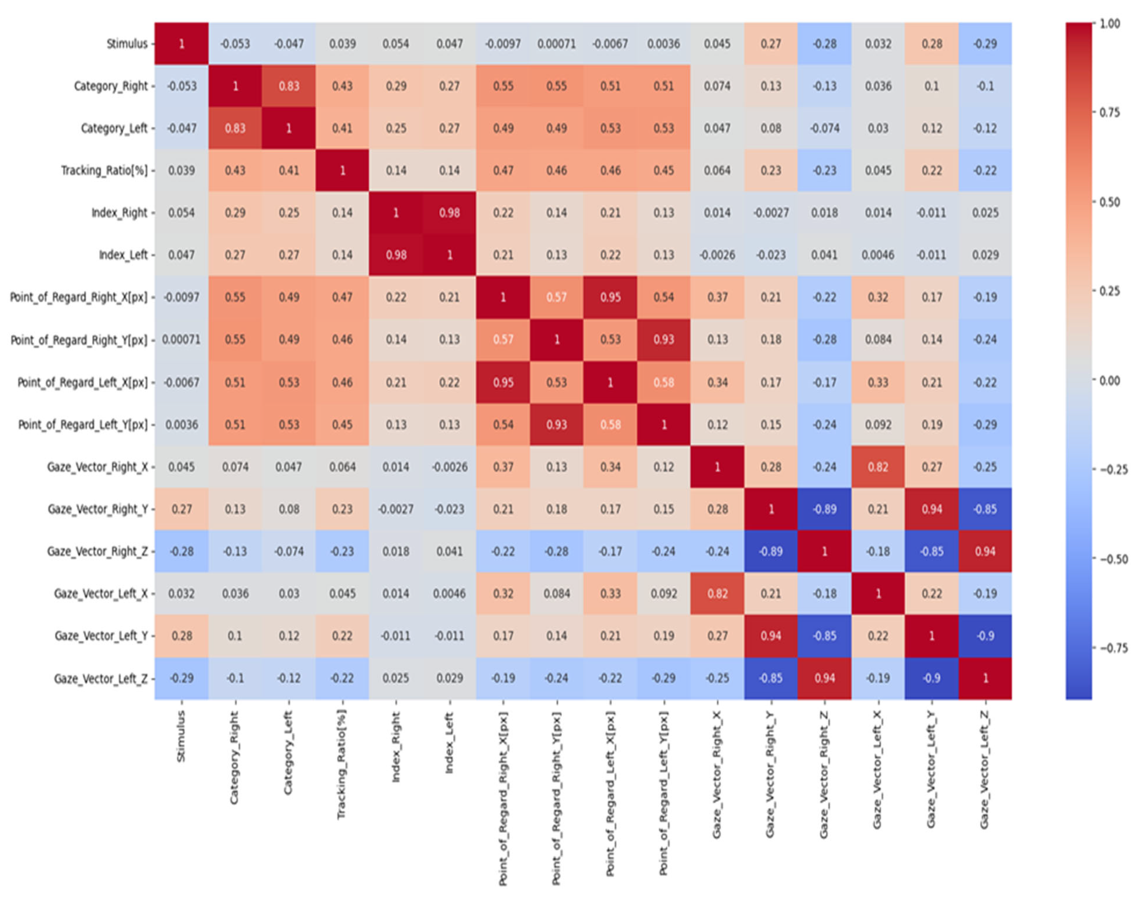
Our proposed model	30 TD and 29 ASD at age (≈3–13) years		Data preprocessing, features selection	LSTM	Testing accuracy of LSTM 98%

. This can be attributed to the meticulous data preprocessing procedures employed, coupled with the judicious selection of salient features that underscore the distinctions between individuals with autism and those without. The model we have advanced achieved a commendable accuracy of 98% utilising the LSTM methodology.

6. Conclusions

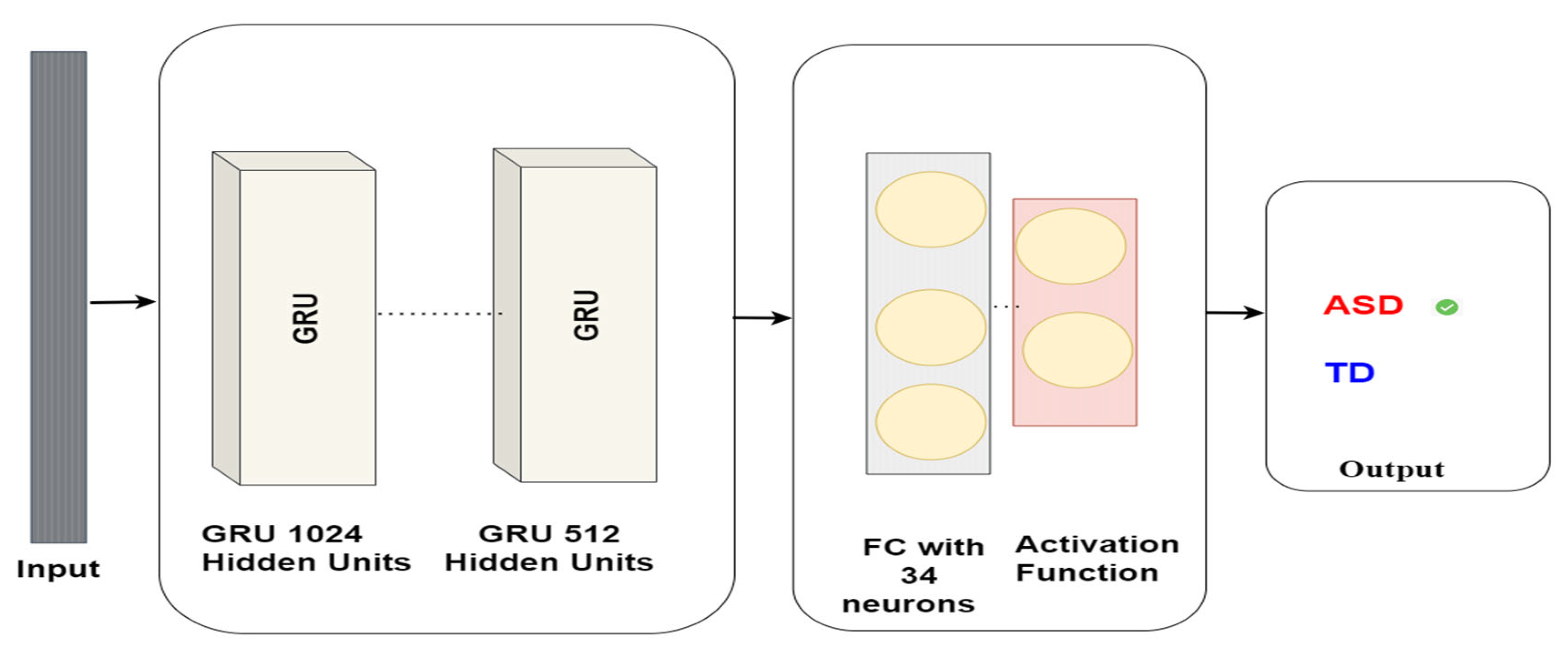
In the dynamic tapestry of contemporary ASD research, this study firmly posits itself as a beacon of innovative methodologies and impactful outcomes. Navigating the intricate labyrinth of ASD diagnosis, the research underscores the critical imperative of early detection, a tenet foundational to effective intervention strategies. At the methodological core lies our deployment of deep learning techniques, uniquely integrating CNN and RNN with an eye-tracking dataset. The performance metrics offer a testament to this integration’s success. Specifically, the BiLSTM yielded an accuracy of 96.44%, the GRU achieved 97.49%, the CNN-LSTM hybrid model secured 97.94%, and the LSTM model notably excelled with an accuracy of 98.33%.

Upon a systematic scrutiny of extant literature, it becomes unequivocally evident that our proposed model stands unparalleled in its efficacy. This prowess can be attributed to our meticulous data preprocessing techniques and the discerning selection of features. It is worth emphasising that the judicious feature selection played a pivotal role in accentuating the distinctions between individuals with autism and their neurotypical counterparts, leading our LSTM model to realize a remarkable 98% accuracy. This research converges rigorous scientific exploration with the overarching goal of compassionate care for individuals with ASD. It reiterates the profound significance of synergising proactive diagnosis, community engagement, and robust advocacy. As a beacon for future endeavours, this study illuminates a path where, through holistic approaches, children with ASD can truly realize their innate potential amidst the multifaceted challenges presented by Autism.

There is a definite path forward for future research to include a larger and more diverse sample, drawing from a larger population of people with ASD and TD individuals. Increasing the size of the sample pool could help researchers spot more patterns and details in the data. Importantly, a larger sample size would strengthen the statistical validity of the results, increasing the breadth with which they can be applied to a wider population.

References

1. Maenner, M.J.; Shaw, K.A.; Bakian, A.V.; Bilder, D.A.; Durkin, M.S.; Esler, A.; Furnier, S.M.; Hallas, L.; Hall-Lande, J.; Hudson, A.; et al. Prevalence and Characteristics of Autism Spectrum Disorder among Children Aged 8 Years—Autism and Developmental Disabilities Monitoring Network, 11 Sites, United States, 2020. MMWR Surveill. Summ. 2023, 72, 1. [Google Scholar] [CrossRef] [PubMed]
2. Øien, R.A.; Vivanti, G.; Robins, D.L. Editorial SI: Early Identification in Autism Spectrum Disorders: The Present and Future, and Advances in Early Identification. J. Autism Dev. Disord. 2021, 51, 763–768. [Google Scholar] [CrossRef]
3. Salgado-Cacho, J.M.; Moreno-Jiménez, M.P.; Diego-Otero, Y. Detection of Early Warning Signs in Autism Spectrum Disorders: A Systematic Review. Children 2021, 8, 164. [Google Scholar] [CrossRef]
4. Zwaigenbaum, L.; Brian, J.A.; Ip, A. Early Detection for Autism Spectrum Disorder in Young Children. Paediatr. Child Health 2019, 24, 424–432. [Google Scholar] [CrossRef] [PubMed]
5. Wan, G.; Kong, X.; Sun, B.; Yu, S.; Tu, Y.; Park, J.; Lang, C.; Koh, M.; Wei, Z.; Feng, Z.; et al. Applying Eye Tracking to Identify Autism Spectrum Disorder in Children. J. Autism Dev. Disord. 2019, 49, 209–215. [Google Scholar] [CrossRef]
6. Galley, N.; Betz, D.; Biniossek, C. Fixation Durations—Why Are They So Highly Variable? Das Ende von Rational Choice? Zur Leistungsfähigkeit Der Rational-Choice-Theorie 2015, 93, 1–26. [Google Scholar]
7. MacKenzie, I.S.; Zhang, X. Eye Typing Using Word and Letter Prediction and a Fixation Algorithm. In Proceedings of the 2008 Symposium on Eye Tracking Research & Applications, Savannah, GA, USA, 26–28 March 2008; pp. 55–58. [Google Scholar]
8. Ahmed, Z.A.T.; Jadhav, M.E. A Review of Early Detection of Autism Based on Eye-Tracking and Sensing Technology. In Proceedings of the 2020 International Conference on Inventive Computation Technologies (ICICT), Coimbatore, India, 26–28 February 2020; IEEE: Piscataway, NJ, USA, 2020; pp. 160–166. [Google Scholar]
9. Kollias, K.-F.; Syriopoulou-Delli, C.K.; Sarigiannidis, P.; Fragulis, G.F. The Contribution of Machine Learning and Eye-Tracking Technology in Autism Spectrum Disorder Research: A Systematic Review. Electronics 2021, 10, 2982. [Google Scholar] [CrossRef]
10. Kang, J.; Han, X.; Hu, J.-F.; Feng, H.; Li, X. The Study of the Differences between Low-Functioning Autistic Children and Typically Developing Children in the Processing of the Own-Race and Other-Race Faces by the Machine Learning Approach. J. Clin. Neurosci. 2020, 81, 54–60. [Google Scholar] [CrossRef] [PubMed]
11. Liu, W.; Li, M.; Yi, L. Identifying Children with Autism Spectrum Disorder Based on Their Face Processing Abnormality: A Machine Learning Framework. Autism Res. 2016, 9, 888–898. [Google Scholar] [CrossRef] [PubMed]
12. Murias, M.; Major, S.; Davlantis, K.; Franz, L.; Harris, A.; Rardin, B.; Sabatos-DeVito, M.; Dawson, G. Validation of Eye-Tracking Measures of Social Attention as a Potential Biomarker for Autism Clinical Trials. Autism Res. 2018, 11, 166–174. [Google Scholar] [CrossRef]
13. Kong, X.-J.; Wei, Z.; Sun, B.; Tu, Y.; Huang, Y.; Cheng, M.; Yu, S.; Wilson, G.; Park, J.; Feng, Z.; et al. Different Eye Tracking Patterns in Autism Spectrum Disorder in Toddler and Preschool Children. Front. Psychiatry 2022, 13, 899521. [Google Scholar] [CrossRef] [PubMed]
14. Yaneva, V.; Ha, L.A.; Eraslan, S.; Yesilada, Y.; Mitkov, R. Detecting Autism Based on Eye-Tracking Data from Web Searching Tasks. In Proceedings of the 15th International Web for All Conference, Lyon, France, 23–25 April 2018; pp. 1–10. [Google Scholar]
15. Eraslan, S.; Yaneva, V.; Yesilada, Y.; Harper, S. Web Users with Autism: Eye Tracking Evidence for Differences. Behav. Inf. Technol. 2019, 38, 678–700. [Google Scholar] [CrossRef]
16. Yaneva, V.; Temnikova, I.; Mitkov, R. A Corpus of Text Data and Gaze Fixations from Autistic and Non-Autistic Adults. In Proceedings of the Tenth International Conference on Language Resources and Evaluation (LREC’16), Portorož, Slovenia, 23–28 May 2016; pp. 480–487. [Google Scholar]
17. Eraslan, S.; Yesilada, Y.; Yaneva, V.; Ha, L.A. ‘Keep It Simple!’: An Eye-Tracking Study for Exploring Complexity and Distinguishability of Web Pages for People with Autism. Univers Access Inf. Soc. 2021, 20, 69–84. [Google Scholar] [CrossRef]
18. Carette, R.; Elbattah, M.; Dequen, G.; Guerin, J.-L.; Cilia, F. Visualization of Eye-Tracking Patterns in Autism Spectrum Disorder: Method and Dataset. In Proceedings of the 2018 Thirteenth International Conference on Digital Information Management (ICDIM), Berlin, Germany, 24–26 September 2018. [Google Scholar]
19. Elbattah, M.; Carette, R.; Dequen, G.; Guérin, J.L.; Cilia, F. Learning clusters in autism spectrum disorder: Image-based clustering of eye-tracking scanpaths with deep autoencoder. In Proceedings of the 2019 41st Annual international conference of the IEEE engineering in medicine and biology society (EMBC), Berlin, Germany, 23–27 July 2019; IEEE: Piscataway, NJ, USA, 2019; pp. 1417–1420. [Google Scholar]
20. Cilia, F.; Carette, R.; Elbattah, M.; Dequen, G.; Guérin, J.L.; Bosche, J.; Vandromme, L.; Le Driant, B. Computer-aided screening of autism spectrum disorder: Eye-tracking studyusing data visualization and deep learning. JMIR Hum. Factors 2021, 8, e27706. [Google Scholar] [CrossRef]
21. Elbattah, M.; Guérin, J.-L.; Carette, R.; Cilia, F.; Dequen, G. Vision-based Approach forAutism Diagnosis using Transfer Learning and Eye-tracking. In Proceedings of the HEALTHINF 2022: 15th International Conference on Health Informatics, Online, 9–11 February 2022; pp. 256–263. [Google Scholar]
22. Elbattah, M.; Guérin, J.-L.; Carette, R.; Cilia, F.; Dequen, G. Nlp-based approach to detect autism spectrum disorder in saccadic eye movement. In Proceedings of the 2020 IEEE Symposium Series on Computational Intelligence (SSCI), Canberra, ACT, Australia, 1–4 December 2020; IEEE: Piscataway, NJ, USA, 2020; pp. 1581–1587. [Google Scholar]
23. Cho, K.W.; Lin, F.; Song, C.; Xu, X.; Hartley-McAndrew, M.; Doody, K.R.; Xu, W. Gaze-Wasserstein: A quantitative screening approach to autism spectrum disorders. In Proceedings of the 2016 IEEE Wireless Health (WH), Bethesda, MD, USA, 25–27 October 2016; IEEE: Piscataway, NJ, USA, 2016; pp. 1–8. [Google Scholar]
24. Kang, J.; Han, X.; Song, J.; Niu, Z.; Li, X. The identification of children with autism spectrum disorder by SVM approach on EEG and eye-tracking data. Comput. Biol. Med. 2020, 120, 103722. [Google Scholar] [CrossRef] [PubMed]
25. Satu, M.S.; Azad, M.S.; Haque, M.F.; Imtiaz, S.K.; Akter, T.; Barua, L.; Rashid, M.; Soron, T.R.; Al Mamun, K.A. Prottoy: A Smart Phone Based Mobile Application to Detect Autism of Children in Bangladesh. In Proceedings of the 2019 4th International Conference on Electrical Information and Communication Technology (EICT), Khulna, Bangladesh, 17–19 December 2019; pp. 1–6. [Google Scholar]
26. Akter, T.; Ali, M.H.; Khan, M.I.; Satu, M.S.; Moni, M.A. Machine Learning Model to Predict Autism Investigating Eye-Tracking Dataset. In Proceedings of the 2021 2nd International Conference on Robotics, Electrical and Signal Processing Techniques (ICREST), Online, 5–7 January 2021; pp. 383–387. [Google Scholar]
27. Akter, T.; Ali, M.H.; Khan, M.I.; Satu, M.S.; Uddin, M.; Alyami, S.A.; Ali, S.; Azad, A.; Moni, M.A. Improved Transfer-Learning-Based Facial Recognition Framework to Detect Autistic Children at an Early Stage. Brain Sci. 2021, 11, 734. [Google Scholar] [CrossRef] [PubMed]
28. Alkahtani, H.; Aldhyani, T.H.H.; Alzahrani, M.Y. Deep Learning Algorithms to Identify Autism Spectrum Disorder in Children-Based Facial Landmarks. Appl. Sci. 2023, 13, 4855. [Google Scholar] [CrossRef]
29. Alkahtani, H.; Ahmed, Z.A.T.; Aldhyani, T.H.H.; Jadhav, M.E.; Alqarni, A.A. Deep Learning Algorithms for Behavioral Analysis in Diagnosing Neurodevelopmental Disorders. Mathematics 2023, 11, 4208. [Google Scholar] [CrossRef]
30. Thabtah, F.; Kamalov, F.; Rajab, K. A New Computational Intelligence Approach to Detect Autistic Features for Autism Screening. Int. J. Med. Inform. 2018, 117, 112–124. [Google Scholar] [CrossRef]
31. Omar, K.S.; Mondal, P.; Khan, N.S.; Rizvi, M.R.K.; Islam, M.N. A Machine Learning Approach to Predict Autism Spectrum Disorder. In Proceedings of the 2019 International Conference on Electrical, Computer and Communication Engineering (ECCE), Bazar, Bangladesh, 7–9 February 2019; pp. 1–6. [Google Scholar]
32. Sharma, M. Improved Autistic Spectrum Disorder Estimation Using Cfs Subset with Greedy Stepwise Feature Selection Technique. Int. J. Inf. Technol. 2019, 14, 1251–1261. [Google Scholar] [CrossRef]
33. Satu, M.S.; Sathi, F.F.; Arifen, M.S.; Ali, M.H.; Moni, M.A. Early Detection of Autism by Extracting Features: A Case Study in Bangladesh. In Proceedings of the 2019 International Conference on Robotics, Electrical and Signal Processing Techniques (ICREST), Dhaka, Bangladesh, 10–12 January 2021; pp. 400–405. [Google Scholar]
34. Erkan, U.; Thanh, D.N. Autism Spectrum Disorder Detection with Machine Learning Methods. Curr. Psychiatry Res. Rev. Former. Curr. Psychiatry Rev. 2019, 15, 297–308. [Google Scholar]
35. Akter, T.; Satu, M.S.; Khan, M.I.; Ali, M.H.; Uddin, S.; Lio, P.; Quinn, J.M.; Moni, M.A. Machine Learning-Based Models for Early Stage Detection of Autism Spectrum Disorders. IEEE Access 2019, 7, 166509–166527. [Google Scholar] [CrossRef]
36. Cilia, F.; Carette, R.; Elbattah, M.; Guérin, J.-L.; Dequen, G. Eye-tracking dataset to support the research on autism spectrum disorder. Res. Sq. 2022. [Google Scholar] [CrossRef]
37. Dasu, T.; Johnson, T. Exploratory Data Mining and Data Cleaning; John Wiley & Sons: Hoboken, NJ, USA, 2003. [Google Scholar]
38. McKinney, W. Python for Data Analysis: Data Wrangling with Pandas, NumPy, and IPython; O’Reilly Media, Inc.: Sebastopol, CA, USA, 2012. [Google Scholar]
39. Buitinck, L.; Louppe, G.; Blondel, M.; Pedregosa, F.; Mueller, A.; Grisel, O.; Niculae, V.; Prettenhofer, P.; Gramfort, A.; Grobler, J.; et al. API design for machine learning software: Experiences from the scikit- learn project. arXiv 2013, arXiv:1309.0238. [Google Scholar]
40. Chawla, N.V.; Bowyer, K.W.; Hall, L.O.; Kegelmeyer, W.P. SMOTE: Syntheticminority over-sampling technique. J. Artif. Intell. Res. 2002, 16, 321–357. [Google Scholar] [CrossRef]
41. LeCun, Y.; Bengio, Y.; Hinton, G. Deep learning. Nature 2015, 521, 436–444. [Google Scholar] [CrossRef] [PubMed]
42. Graves, A. Generating sequences with recurrent neural networks. arXiv 2013, arXiv:1308.0850. [Google Scholar]
43. Hochreiter, S.; Schmidhuber, J. Long short-term memory. Neural Comput. 1997, 9, 1735–1780. [Google Scholar] [CrossRef]
44. Chung, J.; Gulcehre, C.; Cho, K.; Bengio, Y. Empirical evaluation of gated recurrent neural networks on sequence modeling. arXiv 2014, arXiv:1412.3555. [Google Scholar]
45. Zhou, P.; Shi, W.; Tian, J.; Qi, Z.; Li, B.; Hao, H.; Xu, B. Attention-based bidirectional long short-term memory networks for relation classification. In Proceedings of the 54th Annual Meeting of the Association for Computational Linguistics, Berlin, Germany, 7–12 August 2016; Volume 2, Short Papers. pp. 207–212. [Google Scholar]
46. Abadi, M.; Agarwal, A.; Barham, P.; Brevdo, E.; Chen, Z.; Citro, C.; Corrado, G.S.; Davis, A.; Dean, J.; Devin, M.; et al. {TensorFlow}: A system for {Large-Scale} machine learning. In Proceedings of the 12th USENIX Symposium on Operating Systems Design and Implementation (OSDI 16), Savannah, GA, USA, 2–4 November 2016; pp. 265–283. [Google Scholar]
47. Hossin, M.; Sulaiman, M.N. A review on evaluation metrics for data classification evaluations. Int. J. Data Min. Knowl. Manag. Process 2015, 5, 1. [Google Scholar]
Figure 1. The proposed methodology of eye tracking for autism detection.
Data 08 00168 g001
Figure 2. The importance of feature scores.
Data 08 00168 g002
Figure 3. The distribution of features.
Data 08 00168 g003
Figure 4. The correlation coefficient.
Data 08 00168 g004
Figure 5. The number of samples in class TD and ASD.
Data 08 00168 g005
Figure 6. LSTM model architecture for autism detection.
Data 08 00168 g006
Figure 7. CNN-LSTM model architecture for autism detection.
Data 08 00168 g007
Figure 8. GRU model architecture for autism detection.
Data 08 00168 g008
Figure 9. BiLSTM model architecture for autism detection.
Data 08 00168 g009
Figure 10. The confusion matrix of BiLSTM model.
Data 08 00168 g010
Figure 11. The training and testing accuracy and loss of BiLSTM model: (a) accuracy; (b) loss.
Data 08 00168 g011
Figure 12. The confusion matrix of GRU model.
Data 08 00168 g012
Figure 13. The training and testing accuracy and loss of GRU model.
Data 08 00168 g013
Figure 14. The confusion matrix of CNN-LSTM model.
Data 08 00168 g014
Figure 15. The training and testing accuracy and loss of CNN-LSTM model: (a) accuracy; (b) loss.
Data 08 00168 g015
Figure 16. The confusion matrix of LSTM model.
Data 08 00168 g016
Figure 17. The training and testing accuracy and loss of LSTM model: (a) accuracy; (b) loss.
Data 08 00168 g017
Figure 18. The competitive performance of deep learning models.
Data 08 00168 g018