Abstract
In this article, a dataset is described which combines wind turbine supervisory control and data acquisition (SCADA), meteorological and acoustical data and thus gives a detailed description of a wind farm and its atmospheric and acoustic environment. The data were collected during different seasons for several weeks at a time, such that a multitude of environmental and operational conditions are covered. In five measurement campaigns, in total three different locations with similar surroundings were captured. The raw data were enhanced with derived values such as atmospheric stability or direction of sound propagation. Data of one month including all time series measurements as well as monophonic audio recordings are now published. The dataset also contains three exemplary use cases along with documents that describe the data pre-processing.
DataSet: https://doi.org/10.25835/c2mv3d7z.
DataSet License: CC-BY-NC
1. Summary
The investigation of wind turbine operation under various external influences is still ongoing and attracts a significant amount of interest, now that the spotlight is turned more and more on renewable energies due to the energy and climate crisis. One of the points of research is the sound generation and propagation during operation. Another relevant topic is the psychoacoustic influence of the sound on humans. There are several reasons for making our data available. First, the recording procedure is very time-consuming; therefore, we want to save other researchers some time effort. To the best of the authors’ knowledge, there is no dataset available which includes different types of recordings. The dataset at hand combines acoustical, meteorological, and wind turbine supervisory control and data acquisition (SCADA) data. Thus, it could be of interest for different research applications, such as listening tests and data analysis in the field of sound propagation.
1.1. Predecessor Project “WEA-Acceptance”
The dataset described in this paper arose from the project “WEA-Acceptance–from Acoustic Source to Psychoacoustic Assessment” in which, in recent years, a significant number of recordings close to wind turbines were collected. “WEA” in the project name stands for the abbreviation of the German word for wind turbine. The aim of “WEA-Acceptance” was to create a model for predicting wind turbine emissions, sound propagation, and perception of residents. One important factor, especially for the employed listening tests, was to maintain ecological validity. Due to this and in particular to validate the models, extensive acoustical measurements were performed in the area of wind farms. In total, five measurement campaigns, covering all seasons, were executed. Acoustical, meteorological, and SCADA data were recorded over several weeks at a time. Additionally, over 70 short-term acoustical and visual recordings were carried out. Three different measurement locations were recorded per site in the same direction from the turbine, but increasing distances were used for the long-term recordings. For the short recordings, a variety of distances and angles to the turbines were chosen. A summary of the long-term recordings, including season, duration, and used measurement stations, can be found in Table 1. All measurements make use of microphones (MIC), and SCADA data from a number of wind turbines (WTs). In case of location two and three, the data of a 100 m meteorological mast (MET100) were also available. An overview schematic of all utilized equipment is given in Figure 1.

Table 1.
Overview of the continuous measurements of the five measurement campaigns.
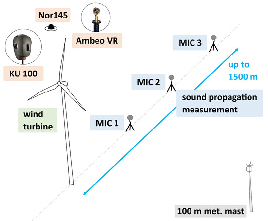
Figure 1.
A schematic overview of the utilized measurement equipment. The equipment in orange was used for the short recordings only, while the rest was used in the long-term measurements.
All recording locations lie within northern Germany and can be categorized as homogeneous flat land with agricultural use. The fields surrounding the wind turbines are separated by ditches, which can contain water.
The data recorded were already used for various investigations. The short-term audio together with 360° video recordings were used for different laboratory studies in the past [1,2]. The results of one of the listening tests were used together with derived perceptional parameters from the used audio to create a model to make a prediction on the potential annoyance of the stimuli [3]. To ensure ecological validity in the laboratory, some investigations were made regarding the audio reproduction using higher order ambisonics by comparing psychoacoustical cues of the original recordings and re-recordings [4]. Furthermore, an algorithm by Pieren and Heutschi to synthesize wind turbine sound [5] was analyzed regarding an extension to create binaural signals [6]. Another investigation of the data was to analyze the soundscape captured in the audio recordings by training a convolutional neural network (CNN) to classify 12 different sound categories. The conceptualizing, training, and validation of the CNN is described in [7]. During “WEA-Acceptance”, the sound pressure level (SPL), meteorological, and SCADA data were used to validate a sound propagation model based on the Crank–Nicolson Parabolic Equations method [8], as well as to investigate the propagation of wind turbine sound based on measured data. For various measurement campaigns, the influence of environmental and operational parameters on the acoustical data were examined. In addition to evaluation methods [9,10], the examinations focused in particular on refraction effects [11,12]. To automate the classification of the acoustical data, the use of k-means clustering on the operational parameters was investigated [13].
1.2. Follow-Up Project “WEA-Acceptance Data”
Whilst the recordings were used by the institutes involved for some research purposes, most of the acquired data were left untouched. In the follow-up project “WEA-Acceptance Data—Database for benchmarking and validation”, more than 13 TB of data were processed such that they would be well-documented and could be used easily by others. Furthermore, the data were made publicly available following the FAIR principles [14]. The concept for this endeavor was presented at different conferences [15] as well as a preview of the contents of the dataset [16]. The investigation of sound classification was followed up by applying the same CNN on the data from a different measurement campaign and comparing the results with other, simpler and less computational-heavy methods, as seen in [17].
1.3. About This Paper
In this paper, a thorough description of our measurement data, the applied methods, and the recording equipment is provided. More details about the recorded data and the contents of the different files can be found in the according subsections of Section 2 including in-depth descriptions of added enhanced data. The measurement setup, used equipment, and the processing of the raw data are described in Section 3. In Section 4, some information on the data availability is given and the provided exemplary use cases are listed.
In the following, only one month of data from measurement campaign five is regarded.
2. Data Description
The dataset includes different kinds of data: audio and tabular. Originally, the audio files were saved as .wav, but they were converted to .flac for a lossless compression. All tabular time series recordings were saved as .parquet, because it uses less disk size than .csv and can be opened in common data analysis languages like Python, R, and Matlab with a single command each. The time series data are split thematically into three: acoustical data, like (relative) sound pressure levels and one-third-octave bands; meteorological data; and SCADA data of the turbines in focus as well as neighboring turbines. All the time series files have the column “Time”, which holds the time stamp of the recording converted to UTC. Using these, it is possible to match and combine the different files.
2.1. Metadata
The file “metadata.json” gives an overview of the measurement location and stations. This includes data on the sensors like height, unit of measurement, and, if applicable, limits for valid value ranges that were used during data cleaning, as described in Section 3.3. For the sensors, it is also stated which columns hold their measurements. Information on the distance and direction to the wind turbine in focus is also given. For the windscreens of the microphones, insertion loss values for each frequency band are noted.
2.2. Acoustical Data
The Institute of Structural Analysis of the Leibniz University Hannover set up three microphones at different distances from the turbine in focus, but in a similar angle. The one nearest to the turbine was placed in the distance of the hub height plus half of the rotor diameter, according to the distance prescribed by IEC 61400-11 [18]. All three microphones recorded a mono audio signal with 51.2 kHz, the A- and Z-weighted sound pressure levels as well as Z-weighted one-third octave bands from 6.3 Hz to 20 kHz, as averages of 1 sec intervals each. In the present dataset, the SPL and octave band values were regrouped into 10 min intervals to have a better compatibility with the other data, which were only provided in 10 min time steps. For a valid value, at least 50% of the interval had to hold valid data; otherwise, it was set to NaN. Furthermore, percentile levels with were added for A- and Z-weighted SPL. This results in three microphone files with 53 columns each. The SPL values had to be anonymized as described in Section 3.4. Descriptions on how they can be nevertheless used are given in Section 4. Except for the “Time” column, all columns are thus given in dBREF. The audio files were down-sampled to 32 kHz to save storage space and are provided as one zipped file per day containing the recordings split into 30 min files grouped by microphone.
2.3. Meteorological Data
During measurement campaigns two to five, we were provided with data from a preinstalled 100 m mast. It was equipped with eight wind speed, three wind direction, two temperature, two humidity, and one pressure sensors at different heights, according to Table 2.
Table 2.
Overview of meteorological data measured at the 100 m mast by height.
Horizontal wind speed is measured in two different directions at each height, with a north–west and a south–east facing cup, while all other sensors are only placed once per height. For all sensors, mean and standard deviation are given in 10 min intervals. For wind speed measurements, the minimum and maximum are given additionally. The column “Rain flag” is a Boolean indication of rainfall. Comparing this to the daily data from a weather station about 2 km east of the mast, the rainfall ranged from 0.2 mm to 8.2 mm on the rainy days. Furthermore, a set of (horizontal and vertical) wind speeds and directions from ultrasonic is given. To enhance the data of the measurement mast, the atmospheric stability was classified according to Table 3 by calculating the wind shear exponent using the mean horizontal wind speeds at 29 m and 100 m height with the equation
with being the mean horizontal wind speed in m/s of the north–west-facing cup and being the height z of the sensor in meters. Both and the stability class were added to the data as their own columns.
Table 3.
Criteria for stability classes in dependence of the wind shear exponent , according to van den Berg [19].
Other additions are the “sound propagation direction” and “relative wind direction”. Both compare the wind direction at 96 m at the meteorological mast against the averaged angle of the three microphones relative to the wind turbine in focus and categorize the resulting direction offset in five different classes as described in Table 4. The “sound propagation direction” and the “relative wind direction” point in exactly opposite directions.
Table 4.
Offset angle ranges of the relative wind direction and sound propagation direction classes, assuming the microphone position at .
2.4. SCADA Data
SCADA data were available for the turbine in focus as well as for turbines in close vicinity to the microphone positions with a resolution of 10 min. The contents of the SCADA files are described in Table 5.
Table 5.
Columns of the SCADA files.
Operation and maintenance (O&M) reports were not provided except for two turbines during measurement campaign five, which were not the one in focus. Thus, the operating states of the turbines were derived from the available SCADA data and saved in the column “operating state”. The state was deduced from the raw, non-normalized data and additional information about the turbine models, like rated power, wind speed, and rotor speed, were used.
Based on the classification of Do and Huang in [20], the following states were considered and applied in the given order: STOP, PARTIAL STOP, CURTAILMENT, PARTIAL CURTAILMENT, OUTLIER, NORMAL. There was no value-related definition given for the states and the transitions between them were not defined, so they were newly determined analyzing the power curves of our dataset. The relationship between these states is illustrated in Figure 2 and described in more detail in the following. An exemplary power curve plot of normalized “power output” values over “wind speed” classified by “operating state” is shown in Figure 3.
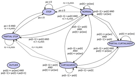
Figure 2.
The state transition diagram for determining the operating states based on observations in the dataset. The following values are abbreviated: po = “power output”; rs(,min) = “(minimal) rotor speed”; pc[ws] = “manufacturer’s power curve value for the wind speed bin”; t = “timestamp”. Dashed arrows show state transitions that likely only occur due to the big averaged time intervals in the present data.
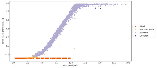
Figure 3.
The deduced operating states of WT1 during measurement campaign 5. Blue squares denote the state STOP, orange stars the state PARTIAL STOP, green triangles the state NORMAL, and red circles the state OUTLIER. During the time of measurement, no curtailment was applied, so these states are not depicted.
STOP
Initially, all measurements with “power output” are classified as STOP. It was considered also looking at the “rotor speed”, but it was rarely 0 at all. However, it can be said that the “rotor speed” stays below the minimal rotor speed according to the manufacturer “rs,min” of the wind turbine model during periods of no “power output”.
PARTIAL STOP
PARTIAL STOP denotes the state in-between STOP and NORMAL in which the turbine starts running, or, in reverse, in which the turbine stops running, but momentum has it still moving. The transition from (PARTIAL) STOP to NORMAL is reached when the “rotor speed” is bigger than the minimal rotor speed “rs,min” of that wind turbine model. It is assumed that the “power output” increases during the transition. Equivalently, the transition between NORMAL and PARTIAL STOP is reached as soon as the “rotor speed” drops below the minimal rotor speed. The “power output” decreases and as soon as it drops to or below zero, the state changes to STOP. A state labelled as PARTIAL STOP can also include a short stopping of the wind turbine, since the data are averages of 10 min intervals.
CURTAILMENT
CURTAILMENT is a state wherein the turbine is running for some time at a fixed “power output”, even though with the given wind condition a higher output could be yielded. This state can be described by having (almost) constant “power output” values (>0) for successive points in time, which lie also distinctly (more than 5% of the rated power) below the manufacturer’s power curve. It can be observed that during CURTAILMENT the “blade pitch” is higher than in NORMAL operation (, ).
PARTIAL CURTAILMENT
Similar to PARTIAL STOP, this state describes the change between CURTAILMENT and NORMAL operation, during which the “blade pitch” is regulated and the “power output” values change to the values expected for the given “wind speed”.
OUTLIER
Data points that were not classified with the preceding categories and have a “power output” value that is much smaller than the value of the manufacturer’s power curve for the current “wind speed”. OUTLIER points are completely unrelated with the “power output” values of the previous and next timestamp and also tend to come with high “blade pitch” values (). It is possible that, in the time period of these data points, there was a rather short shut down of the machine. In the end, a trade-off has been made where points with an Euclidean distance to the manufacturer’s power curve greater than the mean Euclidean distance of all potentially NORMAL states plus three times the standard deviation of the Euclidean distance are classified as OUTLIER. These data points are also characterized by higher “blade pitch” values than truly NORMAL states in their respective bin of “rated wind speed” ± 0.25 m/s. However, this can be prone to misclassification, as the distribution of the measurements is not always coherent with the available manufacturer’s power curve for that turbine, e.g., when the turbine is old.
NORMAL
Any data points not labeled so far are close to the manufacturer’s power curve and thus considered as NORMAL, which means that the turbine produces as much power as expected for the current wind speed.
To verify the algorithm described, a comparison of the O&M logs and the classification results was performed. The logs, however, only state three different states: “running”, “stopped”, and “error”. In the last state, at least in the data available, the turbine was not running, so it was treated as “stopped” as well. Both NORMAL and STOP, were classified correctly over 90% of the time. As a state such as PARTIAL STOP does not exist in the original logs, the results are not entirely correct. A misclassification of NORMAL instead of STOP happens in approximately 5.35% of the cases and the other way in 8.3%. The logs are not always continuous, resulting in 3.8% and 8.1% of the data points not being classified as either of the two.
3. Methods
3.1. General Measurement Setup
A general overview of the devices used in the measurement setup generally can be seen in Figure 1, while a schematic map of location three during the last measurement campaign is shown in Figure 4. The nearest bigger road is in approximately 1 km distance in the south–westerly direction. In each measurement campaign, three microphones were used. The one nearest to the turbine was placed in the distance of the hub height plus half of the rotor diameter, according to the distance prescribed by IEC 61400-11 [18]. The microphones were placed in one line in the same direction from the turbine. During placement, it was made sure that a distance of at least 10 m from bigger vegetation such as trees and bushes was kept to reduce wind-induced vegetation noise. Further reasoning of the measurement setup is given in [9]. A fixed meteorological measuring mast of 100 m height is situated in the area of the wind farm. Finally, the SCADA data of the turbines in the close vicinity to the acoustical stations were made available to us by the operator.
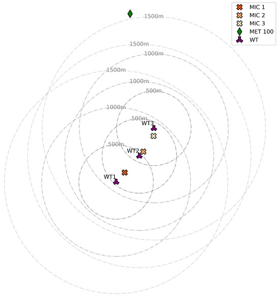
Figure 4.
A schematic map of the measurement site during the measurement campaign. The green diamond stands for the 100 m meteorological mast, the red to yellow hued crosses are the acoustical measurement stations, and the purple symbols surrounded by dashed circles indicating distances are the wind turbines.
Information about the height and distances of all measurement stations is listed in Table 6.
Table 6.
A description of the measurement stations used during measurement campaign five in terms of height and distance to the wind turbine in focus.
3.2. Equipment
The mobile measurement setup of the long-term data was placed in the fields surrounding the wind turbines and stayed at the same place during the campaign. It consisted of three acoustical measurement stations, as shown in Figure 5. Each was equipped with a 01dB DUO smart noise monitor, which includes a G.R.A.S. 40CD microphone, a nose cone, the primary windscreen from the manufacturer, and a secondary in-house build windscreen [21]. Secondary wind screens of different diameters, just a primary windscreen, and also a tertiary windscreen setup were evaluated in the lab with a fan as well as in the field in the vicinity of a turbine. The recordings showed that the commercial primary windscreen alone is insufficient to attenuate wind-induced noise, especially in the outdoor setting. The setup with three windscreens has the biggest influence on the acoustic properties. The best result was achieved with the setup with the bigger secondary windscreen, which could reduce the excess noise below 125 Hz by up to 10 dB and where the insertion loss could be compensated using experimentally determined correction values. The microphones were mounted on weighted tripods at 1.70 m height instead of on a sound-hard plate on the floor to reduce the influence of wind-induced vegetation noise from tall grass. The data were recorded without any pre-processing. The equipment was powered by using solar panels (12 V, 150 W) and rechargeable batteries (12 V, 7.2 Ah).
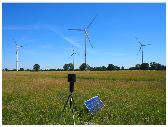
Figure 5.
The measurement site with one of the acoustical measurement stations and its power supply.
The short-term audio recordings for the first exemplary use case (see Section 4) used a set of different microphones. A Neumann KU 100 dummy head equipped with a primary windscreen from Soundman and a secondary in-house built windscreen was used for binaural recordings. Soundfield recordings were made using a Sennheiser Ambeo VR microphone. Three windscreens were used for this microphone: a primary windscreen from Sennheiser made from foam, a secondary DeadCat and a third, self-developed windscreen. Both of these microphones were set to a height of approximately 170 cm. Mono recordings as well as SPL measurements were performed using a Norsonic Nor145 sound-level meter on an acoustically hard plate on the ground with a domed foam windscreen from Norsonic and a secondary hemispherical windscreen made from fabric. The self-developed windscreens were made from brass wire and windproof, but sound-penetrable fabric was investigated in the lab with the result that the acoustic properties were insignificant between 60 and 1000 Hz and in the range of normal measurement tolerances over 1000 Hz. The setup of these recordings can be seen in Figure 6.

Figure 6.
The measurement site with the acoustical measurement stations for short-term recordings.
3.3. Data Treatment
Initially, the raw data were saved in several formats; thus, they were first converted to one common file format. We decided on the parquet format as it shows the best balance of file size and readability in different programming languages. The conversion step also included synchronizing the timestamps, as the different data providers used different time zones as standard. All timestamps were converted to UTC, which results in an offset of one to two hours, depending on the season. At the same time, the data were verified for missing timestamps. These were added and all other columns for these rows were filled with NaN. To obtain an overview of the completeness of the data, an additional table was created, in which the percentage of non-NaN values over all columns is given for each day. This table is updated in the next step, where the data are analyzed for erroneous values and cleaned otherwise. Especially in the SCADA data provided by the operators, there were completely empty columns (e.g., torque) or, in the case of blade pitch, multiple columns (individual blade pitches and averaged blade pitch) with equal values. The former were removed if empty over all campaigns, while the latter were reduced to one column, “blade pitch °”, as all gave the same information. Some columns also needed to be renamed, as they did not have the same name over all measurement campaigns because different operators were involved. Additionally, all values were verified against upper and lower limits, if applicable. All rotational speed values had a lower bound of 0 rpm and an upper bound of the maximal speed according to the turbine model. Both “wind direction” and “nacelle position” had a lower limit of and an upper limit smaller than . The “wind speed” had a lower bound of 0 m/s. Limits for the meteorological data were chosen by verifying the weather report for the duration corresponding to the measurement campaign and applying an uncertainty margin of ±15 hPa and ±5 °C, respectively. Generally, any values outside the limits were set to NaN. The only exception were highly deviant “generator speed” values, as these have a linear relationship of a slope of one with the “gear speed” values. Equation (2) verifies the absolute difference between the two speeds against a threshold relative to the maximal gear speed value (). If it evaluates as false, usually due to very negative “generator speed” () values, said column is set to the corresponding value of “gear speed” ().
If the correlation coefficient between “wind direction” and “nacelle position” equals one, the latter column is set to NaN as it holds no additional information and may have had no own sensor values. Several occurrences of sensor faults happened in the meteorological data; thus, highly negative or constant values were set to NaN.
After cleaning, the data were enhanced with derived values, like “atmospheric stability” for meteorological data and “operating state” for SCADA data, as described in the corresponding sections above.
3.4. Data Anonymization
Finally, according to the wind farm operator, the acoustical and SCADA data had to be anonymized. First of all, the dates of all the files had to be made unrecognizable. To retain the information on season, we kept the month, day, and time as is and only changed the year to 1688, which is near the minimum for Pandas timestamps [22] and evidently not the year of the recording. Some values of the SCADA data had to be normalized, especially the power output and any speed values, using
where is the mean and the standard deviation of the column, x denotes the individual measurement, and z is the normalized value.
The acoustical data had to be anonymized too, as we were not allowed to publish the true loudness values. The reference sound pressure for calculating the sound pressure level is changed. In air, the common reference is 20 μPa, but the new reference value is the sound pressure , which is derived from the immission-relevant maximum sound power level listed in the acoustical report of the turbine in focus (WT1). For the anonymization of the time signals , the sound pressure is referred to the new reference value as well as an arbitrary factor k:
The factor k was added to avoid misinterpretation, i.e., possible confusion with real values.
4. User Notes
We decided to only upload the data of one month of measurement in campaign 5. The rest of the data are prepared as well and available upon request.
The anonymization of the audio and SPL data does not make them unusable as, for example, investigations on amplitude modulation or directivity can still be conducted, because only the loudness value is affected.
As exemplary uses of the data, three use cases are provided, including results and documentation. The first use case addresses finding suitable audio data for listening tests and provides the results of a sound classification using a neural network, as reported in [17]. The second use case concerns validating a propagation model for the prediction of wind turbine sound. The third use case discussed the influence of different environmental conditions on the sound propagation.
Two different solutions for determining the presence or absence of different sound sources using examples from this dataset are described in [17]. If the use case involves investigating only the sound propagation of one turbine, the dataset includes recordings where the other two turbines were shut down and only the one in focus was active.
Author Contributions
Conceptualization, S.P.; methodology, D.S.; software, D.S.; validation, D.S.; formal analysis, D.S.; investigation, D.S.; resources, S.P.; data curation, D.S.; writing—original draft preparation, D.S.; writing—review and editing, D.S., S.P. and J.P.; visualization, D.S.; supervision, J.P.; project administration, J.P.; funding acquisition, J.P. All authors have read and agreed to the published version of the manuscript.
Funding
This research was funded by the Federal Ministry for Economic Affairs and Climate Action by an act of the German Parliament grant number 03EE3062 (WEA-Acceptance Data) and 0324134A (WEA-Acceptance). The Institute of Communications Technology and the Institute of Structural Analysis are part of the Center for Wind Energy Research For-Wind.
Institutional Review Board Statement
Not applicable.
Informed Consent Statement
Not applicable.
Data Availability Statement
The above-mentioned one month of data can be freely downloaded at https://doi.org/10.25835/c2mv3d7z (accessed on 22 February 2024) under Creative Commons Attribution-NonCommercial 3.0. For additional data, please contact the authors.
Acknowledgments
The authors thank both operators for kindly supplying us with the meteorological and SCADA data and allowing us to publish them. The authors would also like to thank the Institute of Structural Analysis of Leibniz University Hannover for planning and performing the long-term acoustic measurements. Thank you for the comments and discussions regarding the measurement data.
Conflicts of Interest
The authors declare no conflicts of interest. The funders had no role in the design of the study; in the collection, analyses, or interpretation of data; in the writing of the manuscript; or in the decision to publish the results.
Abbreviations
The following abbreviations are used in this manuscript:
| CNN | convolutional neural network |
| FAIR | findable, accessible, interoperable, reusable |
| MET | meteorological mast |
| MIC | microphone |
| NaN | not a number—equivalent to an empty/non-existent entry |
| O&M | operation and maintenance |
| SCADA | supervisory control and data acquisition |
| SPL | sound pressure level |
| WT | wind turbine |
References
- Preihs, S.; Bergner, J.; Schössow, D.; Peissig, J. Assessing Wind Turbine Noise Perception by means of Contextual Laboratory and Online Studies. In Proceedings of the 9th International Conference on Wind Turbine Noise, e-Conference from Europe, Online, 18–21 May 2021; pp. 331–344. [Google Scholar]
- Schössow, D.; Kawczynski, D.; Preihs, S.; Peissig, J. Der Einfluss visueller Präsentationsmodi auf die Wahrnehmung von WEA-Stimuli in Probandenstudien. In Proceedings of the Fortschritte der Akustik—DAGA 2023, 49. Jahrestagung für Akustik, Hamburg, Germany, 6–9 March 2023; pp. 534–537. [Google Scholar]
- Preihs, S.; Bergner, J.; Schössow, D.; Peissig, J. On Predicting the Perceived Annoyance of Wind Turbine Sound. In Proceedings of the Fortschritte der Akustik—DAGA 2021, 47. Jahrestagung für Akustik, Vienna, Austria, 15–18 August 2021; pp. 1589–1592. [Google Scholar]
- Bergner, J.; Preihs, S.; Peissig, J. Investigation on Ecological Validity within Higher Order Ambisonics Reproductions of Wind Turbine Noisescapes. In Proceedings of the INTER-NOISE and NOISE-CON Congress and Conference 2019, Madrid, Spain, 16–19 June 2019; pp. 3635–3646. [Google Scholar]
- Pieren, R.; Heutschi, K.; Müller, M.; Manyoky, M.; Eggenschwiler, K. Auralization of wind turbine noise: Emission synthesis. Acta Acust. United Acust. 2014, 100, 25–33. [Google Scholar] [CrossRef]
- Preihs, S.; Bergner, J.; Peissig, J. Ansätze zur binauralen Erweiterung einer Algorithmik zur lästigkeitsbezogenen Analyse und Synthese der Schallemissionen von Windenergieanlagen. In Proceedings of the Fortschritte der Akustik—DAGA 2019, 45. Jahrestagung für Akustik, Rostock, Germany, 18–21 March 2019; pp. 315–318. [Google Scholar]
- Poschadel, N.; Gill, C.; Preihs, S.; Peissig, J. CNN-based multi-class multi-label classification of sound scenes in the context of wind turbine sound emission measurements. In Proceedings of the INTER-NOISE and NOISE-CON Congress and Conference 2021, Washington, DC, USA, 1–5 August 2021; pp. 2687–2698. [Google Scholar] [CrossRef]
- Könecke, S.; Hörmeyer, J.; Bohne, T.; Rolfes, R. A new base of wind turbine noise measurement data and its application for a systematic validation of sound propagation models. Wind Energy Sci. 2023, 8, 639–659. [Google Scholar] [CrossRef]
- Martens, S.; Bohne, T.; Rolfes, R. An evaluation method for extensive wind turbine sound measurement data and its application. Proc. Meet. Acoust. 2020, 41, 040001. [Google Scholar] [CrossRef]
- Martens, S.; Bohne, T.; Rolfes, R. Analyzing the Sound Propagation of Wind Turbines Based on Measured Acoustical and Meteorological Parameters. In Proceedings of the Fortschritte der Akustik—DAGA 2019, 45. Jahrestagung für Akustik, Rostock, Germany, 18–21 March 2019; pp. 311–314. [Google Scholar]
- Martens, S.; Bohne, T.; Rolfes, R. Measuring and Analysing the Sound Propagation of Wind Turbines. In Proceedings of the 8th International Conference on Wind Turbine Noise, Lisbon, Portugal, 12–14 June 2019; pp. 384–396. [Google Scholar]
- Martens, S.; Bohne, T.; Rolfes, R. Entfernungsabhängige Refraktionseffekte in der Schallausbreitung von Windenergieanlagen. In Proceedings of the Fortschritte der Akustik—DAGA 2020, 46. Jahrestagung für Akustik, Hanover, Germany, 16–19 March 2020; pp. 472–475. [Google Scholar]
- Martens, S.; Findeisen, L.; Bohne, T.; Rolfes, R. Automatisiertes Clustering der Schallemissionen von Windenergieanlagen. In Proceedings of the Fortschritte der Akustik—DAGA 2021, 47. Jahrestagung für Akustik, Vienna, Austria, 15–18 August 2021; pp. 1548–1551. [Google Scholar]
- FAIR Principles. Available online: www.go-fair.org/fair-principles/ (accessed on 12 September 2023).
- Schössow, D.; Bergner, J.; Preihs, S.; Peissig, J. Concept for an open database of acoustical wind turbine measurements. In Proceedings of the Poster at WindEurope Technology Workshop 2022, Brussels, Belgium, 23–24 June 2022. [Google Scholar]
- Schössow, D.; Preihs, S.; Peissig, J. WEA-Acceptance Data—A FAIR wind turbine dataset. In Proceedings of the Presentation at Wind Energy Science Conference 2023, Glasgow, UK, 23–26 May 2023. [Google Scholar]
- Schössow, D.; Preihs, S.; Peissig, J.; Könecke, S.; Bohne, T.; Rolfes, R. A comparison of methods for identifying wind turbine sounds in big data sets. In Proceedings of the 10th International Conference on Wind Turbine Noise, Dublin, Ireland, 21–23 June 2023; pp. 374–394. [Google Scholar]
- IEC 61400-11:2012; Wind Turbines—Part 11: Acoustic Noise Measurement Techniques. IEC: Geneva, Switzerland, 2012.
- Van den Berg, F.G.P. Wind turbine power and sound in relation to atmospheric stability. Wind. Energy Int. J. Prog. Appl. Wind. Power Convers. Technol. 2008, 11, 151–169. [Google Scholar] [CrossRef]
- Do, M.T.; Huang, G. Performance Analysis of Wind Farm with SCADA data: From the methodology to a case study. In Proceedings of the Poster at WindEurope Technology Workshop 2022, Brussels, Belgium, 23–24 June 2022. [Google Scholar]
- Martens, S.; Boas, M.; Bohne, T.; Rolfes, R. Towards the use of secondary windscreens to improve wind turbine sound measurements. In Proceedings of the 15th EAWE PhD Seminar on Wind Energy, Nantes, France, 29–31 October 2019. [Google Scholar]
- Minimal Timestamp in Pandas. Available online: https://pandas.pydata.org/pandas-docs/stable/reference/api/pandas.Timestamp.min.html (accessed on 12 September 2023).
Disclaimer/Publisher’s Note: The statements, opinions and data contained in all publications are solely those of the individual author(s) and contributor(s) and not of MDPI and/or the editor(s). MDPI and/or the editor(s) disclaim responsibility for any injury to people or property resulting from any ideas, methods, instructions or products referred to in the content. |
© 2024 by the authors. Licensee MDPI, Basel, Switzerland. This article is an open access article distributed under the terms and conditions of the Creative Commons Attribution (CC BY) license (https://creativecommons.org/licenses/by/4.0/).