
Diapycnal Velocity in the Double-Diffusive Thermocline

Department of Oceanography, Naval Postgraduate School, Monterey, CA 93943, USA
*
Author to whom correspondence should be addressed.
Fluids 2016, 1(3), 25; https://doi.org/10.3390/fluids1030025
Submission received: 22 May 2016
/
Revised: 30 July 2016
/
Accepted: 12 August 2016
/
Published: 25 August 2016
(This article belongs to the Collection Geophysical Fluid Dynamics)
Abstract
:A series of large-scale numerical simulations is presented, which incorporate parameterizations of vertical mixing of temperature and salinity by double-diffusion and by small-scale turbulence. These simulations reveal the tendency of double-diffusion to constrain diapycnal volume transport, both upward and downward. For comparable values of mixing coefficients, the average diapycnal velocity in the double-diffusive thermocline is much less than in the corresponding turbulent regime. The insulating effect of double-diffusion is rationalized using two theoretical models. The first argument is based on the assumed vertical advective-diffusive balance. The second theory uses the Rhines and Young technique to evaluate the net diapycnal transport across regions bounded by closed streamlines at a given density surface. The numerical simulations and associated analytical arguments in this study underscore fundamental differences between double-diffusive mixing and mechanically generated small-scale turbulence. When both double-diffusion and turbulence are taken into account, we find that the constraints on diapycnal velocity loosen (tighten) with the increase (decrease) of the fraction of the overall mixing attributed to turbulence. The range of diapycnal velocities that could be realized in doubly-diffusive fluids is determined by the variation in the heat/salt flux ratio. We hypothesize that the unique ability of double-diffusive mixing to actively control diapycnal volume transport may have significant ramifications for the structure and dynamics of thermohaline circulation in the ocean.
1. Introduction
Theory of heat and mass transfer by small-scale transient motions constitutes a large and important component of numerous physical sciences, including fields as diverse and seemingly unrelated as oceanography, astrophysics, geology and materials science. The key challenge in small-scale mixing theory, in all its forms and applications, is the analysis and prediction of mean turbulent transport for a given large-scale distribution of properties. Most small-scale mixing processes in fluids that are nominally stably stratified—with density decreasing upwards—can be broadly classified into mechanically-driven and double-diffusive categories. An example of a common mechanically-driven phenomenon is the intermittent generation of small-scale turbulence by shear associated with internal gravity waves. Double-diffusive phenomena, on the other hand, are caused by unequal molecular diffusion rates of two (or more) individual density components, such as temperature and salt in the oceanic context.
Recent years have witnessed a substantial progress in our understanding of both double-diffusive and turbulent phenomena. In particular, reliable parameterizations have been developed for double-diffusion in astrophysical [1,2] and oceanographic [3] contexts. These parameterizations express the vertical fluxes of diffusing properties as a function of the corresponding large-scale gradients using Fick’s diffusion model:
where the eddy diffusivities themselves are not uniform but assumed to depend on the density ratio , where are the expansion/contraction coefficients.
The purpose of this communication is to discuss one fundamental yet mostly overlooked distinction in the dynamics and consequences of double-diffusive and mechanically-driven mixing. In addition to the vertical transport of diffusing properties (e.g., temperature and salinity) which the flux-gradient laws (Equation (1)) attempt to represent, numerous applications require knowledge of the corresponding volume or mass transport across mean density surfaces. Following oceanographic nomenclature, the velocity component normal to the density surfaces () will be referred to as the diapycnal velocity and the associated volume flux as the diapycnal transport. It is the analysis of diapycnal transport which reveals some rather unique properties of double-diffusion that have no direct counterpart in one-component turbulent flows. In particular, we argue that in double-diffusive flows, diapycnal volume transport is dramatically reduced relative to that in turbulent systems with comparable mixing rates of density components. When both double-diffusion and turbulence are present, diapycnal velocity is restricted to a finite range, which is controlled by the relative contributions of double-diffusion and turbulence to overall mixing.
Much of the motivation for the analysis of diapycnal volume transport [4,5,6,7] stems from the role it plays in the theory of thermohaline circulation in the ocean. Thermohaline circulation—the system of large-scale flows driven by the sea-water density variation—is an essential regulator of the Earth’s climate. Nevertheless, several aspects of it have not been fully explained. The classical view [8,9,10,11] emphasizes the role of small-scale mixing and associated water mass transformation in the ocean interior. This idea was challenged by studies advocating an alternative adiabatic view [12,13,14] which invokes isopycnal advection as the key mechanism for maintenance of the Meridional Overturning Circulation (MOC). While the exact contributions of different circulation components remain a source of debate, there is a general consensus that the diabatic mode, driven by diapycnal fluxes, can be substantial. Radko et al. [15] for instance, estimate that the diabatic mode of circulation accounts for approximately one third of the Meridional Overturning Circulation (MOC) in the global ocean. Another uncertain aspect of the theory of thermohaline circulation concerns the relative role of shallow overturning cells in the main thermocline and deep circulation in the abyssal ocean. Earlier efforts [9,16] were mostly focused on the abyssal dynamics. However, an interesting suggestion was made [17] that the meridional transport of heat is controlled by the processes operating in the upper ocean. In an attempt to quantify partitioning of the oceanic heat flux between the deep and shallow overturning cells, these authors introduced the “heatfunction”, a quantity which identifies the components of circulation which contribute to the total meridional heat flux. Boccaletti et al. [17] have shown that the heatfunction represents a surface-intensified flow largely limited to the main thermocline. Therefore meridional heat transport is dominated by the contribution from the upper branch of the MOC where double-diffusion is most active. For instance, as much as 95% of the Atlantic thermocline is double-diffusively unstable [18]. Thus, the link between double-diffusion and diapycnal volume transport can have potentially critical ramifications for thermohaline circulation and should be explored much further.
In order to rationalize the tendency of double-diffusion to suppress the diapycnal volume transport, we propose two arguments. The first argument applies to the strongly diabatic regime representative of the lower (diffusive) thermocline that is often described by Munk’s [9] vertical advection-diffusion balance. We find that steady one-dimensional solutions in double-diffusive systems are possible only for a very narrow range of diapycnal velocities. The second argument is more relevant for the central thermocline, where double-diffusive processes are most common. Dynamics of the main thermocline are fundamentally three-dimensional [19]. The overall water-mass distribution is set by large-scale advection whereas diapycnal mixing is relatively weak. Nevertheless, in this regime it is still possible to predict the impact of higher order diabatic processes on cross-isopycnal transfer using a technique originally developed by Rhines and Young [20]. The crux of this approach is the integration of governing equations along closed streamlines, which effectively eliminates the zero order advective terms in integral balances. Adapting this procedure to the double-diffusive problem allows us to evaluate the average diapycnal velocity in regions bounded by closed streamlines and, ultimately, to explain the insulation effect from first principles. Thus, for both advectively-dominated and diffusively-dominated regimes, there are theoretical reasons to expect the suppression of diapycnal volume flux by double-diffusion.
The paper is set as follows. Our starting point (Section 2) is an analysis of a one-dimensional vertical advective-diffusive balance of temperature and salinity of Munk’s [9] type. This analysis, albeit highly idealized, suggests that fundamental differences may exist in the way turbulent and double-diffusive mixing affect diapycnal volume transport. Motivated by this possibility, we perform a series of large-scale three-dimensional multi-century numerical simulations (Section 3), which also consistently reflect the tendency of double-diffusion to constrain diapycnal volume transport. In Section 4, we develop an analytical model of the double-diffusive insulation in a three-dimensional setting. We summarize and conclude in Section 5.
2. Preliminary Considerations
Our inquiry into the link between double-diffusive mixing and the associated diapycnal volume transport was originally motivated by the following fairly abstract problem. Consider a one-dimensional model consisting of the steady state temperature and salinity equations:
where and are the large-scale temperature and salinity of the sea-water; is the upward vertical velocity. The temperature and salinity fluxes are attributed to small-scale mixing processes and related to large-scale gradients through Equation (1). We are interested in solving Equation (2) for given boundary conditions:
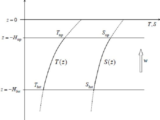
where , () represents the top (bottom) of the mixing zone and is its thickness (see the schematic in Figure 1. In particular, we are concerned by the differences in the solutions of Equations (2) and (3) for cases in which vertical mixing is controlled by: mechanical turbulence, double-diffusion, and a combination thereof.
2.1. Turbulent Mixing
To illustrate the basic properties of the 1D system (Equation (2)), consider first the simplest model of turbulent mixing characterized by constant and equal eddy diffusivities of heat and salt:
In this case, Equations (2) and (3) can be solved for any value of diapycnal velocity ():
and
Thus, the turbulent mixing model (Equation (4)) represents an extreme case of a completely passive system which offers no restrictions on diapycnal velocity. For any value of w it is possible to construct a consistent solution of the T-S advection-diffusion equations satisfying the boundary conditions at and . It should be noted that the advective-diffusive balance (Equation (2)) remains passive even when the diffusivities of heat and salt are spatially uniform but not equal to each other (). The latter model can be used to represent differential diffusion, the preferential turbulent mixing of temperature relative to salinity under certain conditions [21,22]. In order to demonstrate that the passive character of the advective-diffusive balance is not necessarily realized in other types of mixing, we now turn to a very different configuration which demands a unique value of —the constant flux ratio model of double-diffusion.
2.2. Double-Diffusion: The Constant Flux Ratio Model
Double-diffusion comes in two distinct forms, fingering and diffusive convection. The fingering regime is commonly realized in the subtropical thermocline where warm and salty water overlies cold and fresh. Diffusive convection is more prevalent in high-latitude oceans, where temperature and salinity frequently increase downward. While we believe that the analysis in this paper is relevant for both forms of double-diffusion, to be specific, the discussion is focused on the salt-finger regime.
The single most significant parameter controlling diapycnal mixing in regions of active double-diffusion is the local density ratio
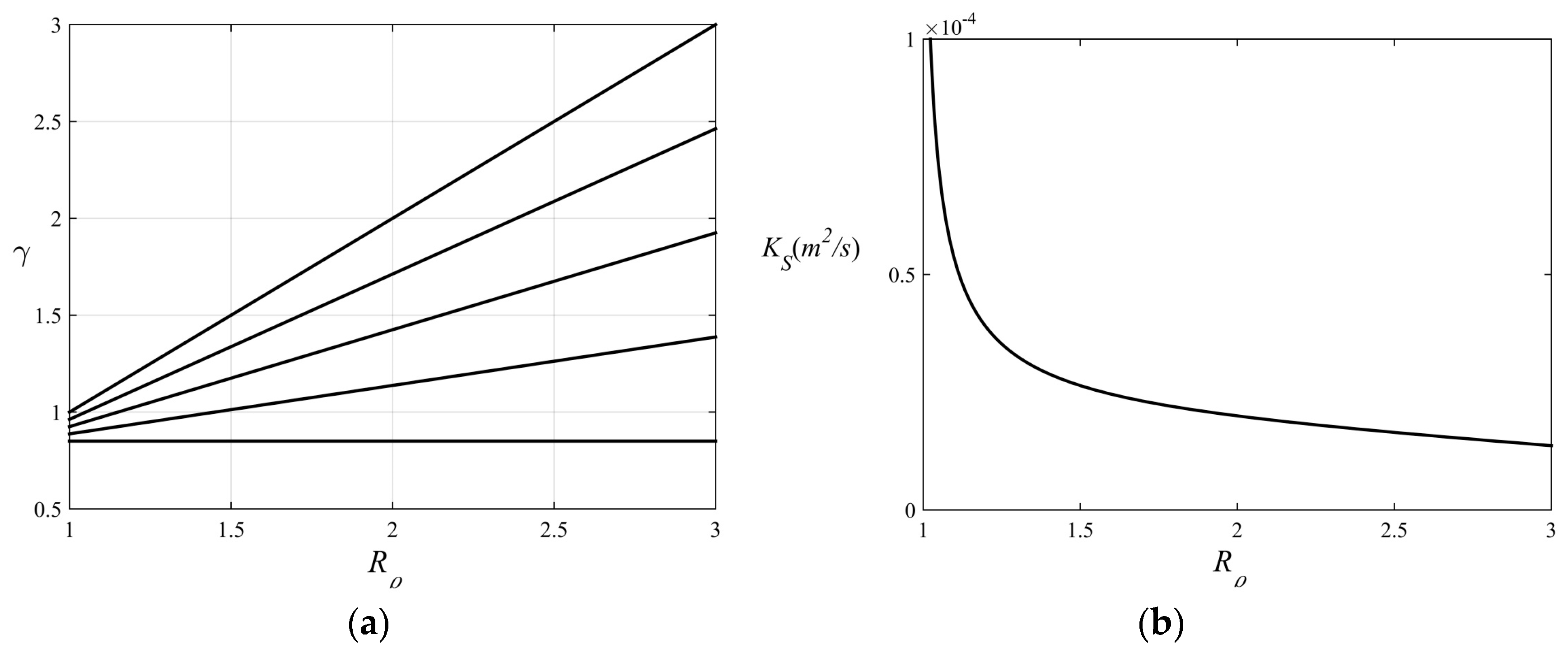
where and are the expansion/contraction coefficients in the linear equation of state—see the discussion in Schmitt [18,23] and Radko [24]. Double-diffusive parameterizations typically assume that the eddy diffusivities of heat and salt are determined by . It is also common to approximate the ratio of thermal and haline density fluxes, so-called flux ratio (), by a constant value:
Particular examples of such parameterizations can be found in, for example, Schmitt [25], Zhang et al. [26], and Merryfield et al. [27].
Combining Equations (2) and (8), we arrive at
To maintain fingering convection, the loss of potential energy stored in salt stratification should exceed the energy gain by heat stratification and therefore . The density ratio, on the other hand, has to exceed unity in order for density to decrease upward. Hence, and therefore Equation (9) can be satisfied only if . Thus, in contrast with the turbulent mixing model, the double-diffusive system actively controls diapycnal velocity. Of course, the selection of a unique in this model could be a consequence of the chosen flux laws; of particular concern is the constant flux ratio approximation (Equation (8)). However, even when the assumption of constant flux ratio is relaxed (Appendix) by considering typical finite variations in we still find that the range of permitted diapycnal velocities is rather narrow: .
2.3. Combined Effects of Double-Diffusion and Turbulence
Because small-scale mixing in the ocean is controlled by a combination of double-diffusion and mechanically generated turbulence, it is of interest to examine the constraints on diapycnal velocity in a model which includes both mixing processes. For that, we extend the foregoing analyses by considering the following closure:
which assumes equal and uniform diffusivities of heat and salt due to turbulence (). Note that this simplified conceptual model does not take into account the possibility of direct influence of turbulence on double-diffusion [28,29].
There have been at least two attempts to evaluate the flux ratio based on oceanographic field measurements [30,31]. Both estimates were mutually consistent, suggesting the flux ratio of
The individual values of salt finger fluxes, and particularly the pattern of their variation with , are more difficult to infer from observations. Therefore, we adopt the parameterization proposed by Radko and Smith [3] on the basis of high-resolution DNS:
where and
We assume parameter values representative of mid-latitude thermocline:
where . Next, we systematically vary in an attempt to determine how it affects the range of diapycnal velocities.
The system consisting of Equation (2) and Equations (11)–(14) was coded in Maple software package and solutions were sought for a range of . Note that in the context of the one-dimensional model, in which all field variables are assumed to vary in z only, the continuity equation reduces to the requirement that . This feature simplifies the exploration of the parameter space and the results are shown in Figure 2. Calculations resulting in regular solutions are indicated by the heavy dots and the light dots represent conditions under which no solutions were found. Figure 2 indicates that the constraints on diapycnal velocity loosen (tighten) with the increase (decrease) in —a quantity measuring the relative contributions from turbulence and double-diffusion to the net mixing.
Despite considerable uncertainties in the estimated magnitudes of double-diffusive and turbulent mixing, it is plausible that in the central thermocline of the Atlantic Ocean their diffusivities are comparable [32]. For we obtain the following constraint on the (dimensional) diapycnal velocity:
which is similar to the data-based estimates of the diapycnal velocity in regions susceptible to both double-diffusive and turbulent mixing [32].
In summary, the foregoing calculations indicate that (i) in the turbulent model, the assumed vertical T-S balances do not impose any internal constraints on diapycnal transport; (ii) in the double-diffusive model the diapycnal transport is zero; and (iii) the hybrid model, which takes into account both double-diffusion and turbulence, allows only a finite range of diapycnal velocities. These findings, of course, should be interpreted with great caution—the ability of any one-dimensional model to reflect the inherently three-dimensional dynamics of ocean circulation is suspect. Perhaps it is most profitable to interpret these one-dimensional solutions as the result of the averaging of the advection-diffusion equations along isopycnal surfaces, although this conceptualization raises the question whether such averaging is physically justified. Nevertheless, the profound differences in the way various mixing models affect diapycnal volume transport provide a compelling reason to launch a more comprehensive investigation of this phenomenon using more realistic—three-dimensional and time-dependent—models. We now proceed with the analysis of double-diffusive insulation based on a series of large-scale numerical simulations.
3. Large-Scale Numerical Simulations
3.1. Formulation
The MIT General Circulation Model (MITgcm), described in [33,34], was used to simulate an ocean of equatorial to sub-arctic meridional extent with a zonal width comparable to that of the North Atlantic. The model solves the incompressible Boussinesq equations of motion with the linear equation of state. The model geometry is a rectangular domain with dimensions
resolved by Cartesian grid points with and . The relatively coarse horizontal resolution prevents generation of mesoscale variability, thereby isolating phenomena of interest—double-diffusive and turbulent diapycnal mixing. Thermohaline forcing is represented by strong relaxation of the surface temperature and salinity to the zonally uniform target patterns shown in Figure 3a,b. The surface temperature and salinity vary linearly with latitude from and to , and . Surface forcing also includes y-dependent zonal wind stress (Figure 3c) prescribed as follows:
where . The variation in the Coriolis parameter (f) is represented by the beta-plane approximation:
where .
The model was initialized from rest with a T-S distribution that is zonally uniform but varies linearly in y and z. The target temperatures and salinities (Figure 3) served as initial surface values as well and initial bottom values were and . The corresponding density ratios monotonically increase from at to at . Horizontal and vertical eddy viscosities were set at and . The nonlocal K-Profile Parameterization (KPP) scheme of Large et al. [35] is used to model convective and near-surface mixing processes. Geostrophic eddy parameterization follows Gent and McWilliams [36]. To reduce spurious interactions with KPP and to isolate the dynamics of interest, the isopycnal diffusivity was set to the minimal value () required to maintain the numerical stability of the model. Vertical mixing of temperature and salinity was represented by a combination of double-diffusion and turbulence. Double-diffusion was parameterized using Equations (12) and (13). The interior turbulent diffusivity () associated with overturning gravity waves, is assumed to be spatially uniform and equal for temperature and salinity. In a series of simulations was systematically varied from 0 to . In the region of western intensification (), however, was maintained at the minimum value of . This restriction was implemented to prevent excessive convection in the regions where the western boundary current, transporting relatively warm and light water northward, enters locations with much higher target surface density. Each simulation was integrated forward for at least 200 years using a time step of 480 s, which was sufficient to produce quasi-steady circulation patterns.
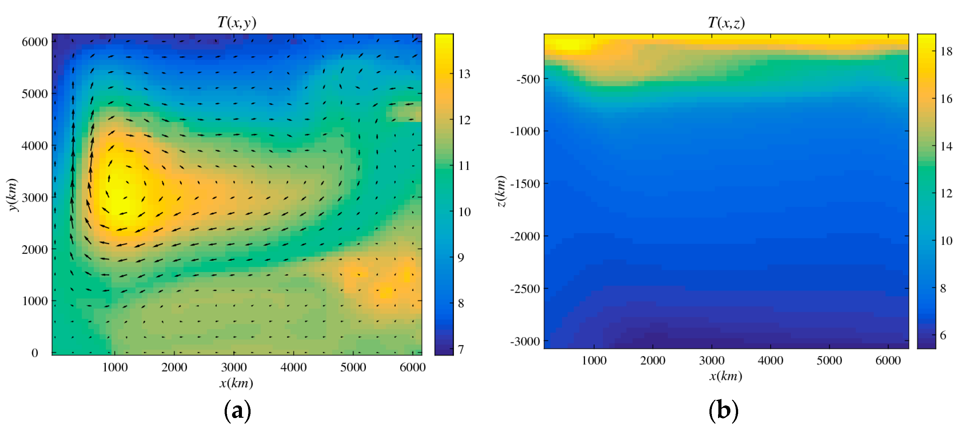
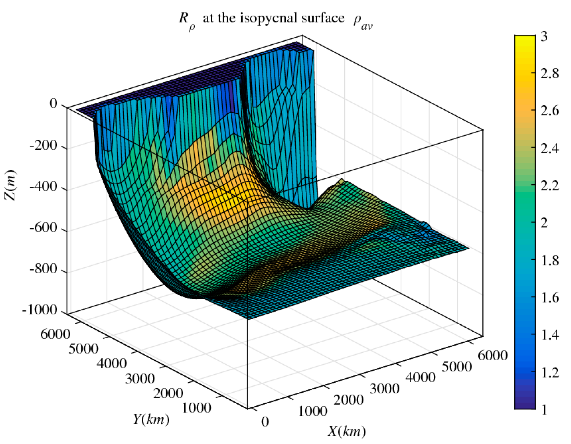
Figure 4 and Figure 5 present a typical final state realized in our numerical experiments. This simulation has been performed assuming purely double-diffusive interior mixing, with for . Figure 4a shows the horizontal temperature distribution and the velocity pattern at . As expected, the flow field is dominated by clockwise circulation in the subtropical region () where wind forcing is anticyclonic. A vertical zonal section of temperature at is shown in Figure 4b. Clearly visible is a well-defined thermocline with relatively warm water extending several hundred meters downward from the surface. Figure 5 presents a three-dimensional view of the isopycnal , where
and () represents the maximal (minimal) density in the computational domain. The color coding represents the values of the density ratio on this isopycnal. The observed range of density ratios indicates that fingering is active on this isopycnal and that its intensity is relatively high.
3.2. Diapycnal Velocity
The analysis in Section 2 pertained to steady one-dimensional systems in which diapycnal volume transport is associated with vertical advection. To quantify diapycnal fluxes in a more realistic three-dimensional setting, the diagnostics of large-scale simulations will be focused on diapycnal velocity [37,38] which is generally dissimilar to the vertical velocity (). Diapycnal velocity can be defined by rewriting governing equations in terms of density (rather than z) as a vertical coordinate:
where
In Equation (21), and represent the slopes of isopycnal surfaces in x and y. For steady-state circulation patterns, Equation (20) reduces to
Figure 6 illustrates the following physical interpretation of diapycnal velocity. Consider a Lagrangian particle initially located at the motionless isopycnal surface (point A). In the presence of a finite cross-isopycnal flow, this particle will be advected by velocity to a new point B, located off the isopycnal. Let C be the vertical projection of the point B onto the isopycnal surface. In this configuration, the diapycnal velocity in Equation (22) represents the rate of increase of the vertical separation of our Lagrangian point from the density surface: . Note that the shadow point C, which remains on the isopycnal, can also alter its z-level and the corresponding vertical velocity can be expressed as
Thus, the isopycnal ascent rate and diapycnal velocity represent two distinct components of vertical velocity:
Equation (22) indicates that in the absence of any diabatic water-mass transformation, and therefore diapycnal velocity is zero. Curiously, the reverse statement is not necessarily correct. The double-diffusive example in Section 2.2 indicates that diapycnal velocity can still be zero even in the presence of substantial diabatic mixing of properties.
An alternative explanation of low diapycnal velocity can be based on the dianeutral velocity equation [4] which, for the conditions assumed in our study, reduces (in present notation) to:
In the case of a purely double-diffusive system, the diapycnal transport is represented by the third term on the right-hand side, which is proportional to . Since the flux ratio in the ocean (Equation (11)) is rather close to unity, relatively low values of diapycnal velocity are expected even when the stratification cannot be accurately described by the predominantly one-dimensional Munk-type model.
The following analysis will therefore attempt to determine whether, and to what extent, is suppressed by double-diffusion in the more realistic three-dimensional systems.
3.3. Diapycnal Transport in the Double-Diffusive and in the Turbulent Ocean
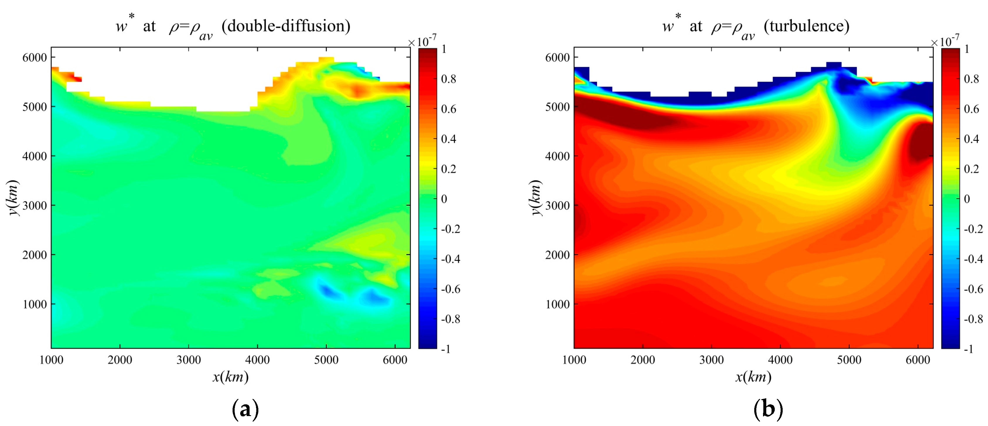
First, the proposed diagnostics have been applied to the double-diffusive experiment shown in Figure 4 and Figure 5. Diapycnal velocity was computed using Equation (22) and evaluated at the isopycnal surface . The results are plotted (Figure 7a) for the interior region () where mixing is exclusively double-diffusive. The same procedure was then applied to the turbulent experiment (Figure 7b). The latter was designed in the same way as the baseline double-diffusive run, except that the vertical mixing was assumed to be exclusively turbulent with
The comparison of diapycnal velocities in these experiments reflects the dramatic difference in the way double-diffusion and turbulence affect diapycnal transport. Over most of the isopycnal surface, the double-diffusive are on the order of or less (both positive and negative values are observed). On the other hand, the turbulent is mostly positive and is larger by at least an order of magnitude (). The difference between Figure 7a,b becomes particularly striking when we recall that typical T-S diffusivities in the two experiments are comparable. For instance, the volume-averaged diffusivities in the double-diffusive experiment are , and these values are similar to the turbulent diffusivity (Equation (26)).
Figure 8a presents the mean diapycnal velocity evaluated at various isopycnal surfaces . In computing , we excluded the contribution from two regions with elevated turbulent diffusivity: (i) the western intensification region () and (ii) the near surface region () where some isopycnal surfaces enter the mixed layer, particularly in the cold Northern parts of the domain. Diapycnal velocity was evaluated for both turbulent and double-diffusive experiments and referenced (Figure 8a) to the average depth of isopycnal surfaces . Figure 8a shows that turbulent diapycnal velocity (blue curve) substantially exceeds the double-diffusive (green curve) for most isopycnals. In both cases, relatively large values of were found at the base of the main thermocline (). Diapycnal velocity in the turbulent experiment was also greatly amplified in the abyssal region () whereas no such amplification occurred in the double-diffusive simulation. It is interesting to note that the patterns of isopycnal-averaged diapycnal velocity are qualitatively similar to the corresponding local vertical profiles. For instance, in Figure 8b we plot the diapycnal velocity profile at the center of the model domain: . Local diagnostics also indicate that the diapycnal velocity in the turbulent ocean greatly exceeds the double-diffusive . Thus, the double-diffusive insulation effect considered in this study represents both the integral and the local property of large-scale flows.
An attempt has also been made to determine the constraints on diapycnal velocity in an ocean experiencing vertical mixing due to a combination of double-diffusion and mechanically generated turbulence. For that, we performed a series of simulations in which was systematically varied, while retaining the parameterization (Equations (11)–(13)) for double-diffusion. Diapycnal velocity was computed and evaluated as previously (Figure 7 and Figure 8). As expected, we find that diapycnal transport intensifies with the increase of the fraction of the overall mixing attributed to turbulence. Figure 9 presents the variation of the isopycnal-averaged diapycnal velocity at the isopycnal surfaces in Equation (19) as a function of . These diagnostics also support our interpretation of double-diffusive mixing as an insulating mechanism. When is less than typical values for and , the overall system behaves like the fully double-diffusive case (e.g., Figure 7a). Values of mean diapycnal velocity are on the order of or less for experiments with Conversely, simulations with are characterized by on the order of or greater.
3.4. The Role of the Flux Ratio
The foregoing experiments have illustrated the dramatic differences in diapycnal volume flux in double-diffusive and turbulent systems. The question that naturally arises at this point is what aspect of double-diffusion makes it so effective in blocking diapycnal volume transport? Theoretical arguments presented in the Appendix suggest that, at least in one-dimensional models, the range of diapycnal velocities is controlled by the effective variation in the flux ratio (). Double-diffusive systems are characterized by a relatively uniform . For instance, Radko and Smith [3] find that as the density ratio increases from to , the flux ratio decreases by . The flux ratio realized in turbulent fluids varies over the same interval much more (), which suggests significantly larger values of diapycnal velocity. In particular, the one-dimensional model (Appendix) predicts that . To determine whether these conclusions remain relevant for three-dimensional systems, we have performed an additional series of four double-diffusive simulations with variable flux ratio patterns.
The new simulations were identical to the baseline double-diffusive experiment (Figure 3 and Figure 4) in all respects except for the chosen flux ratio model, which assumed that varies linearly with the density ratio:
The flux ratio models used in these simulations are shown in Figure 10a, along with the baseline experiment, and the corresponding parameter values are and respectively. The negative values of have not been considered since the decreasing relation results in the formation of thermohaline staircases [39,40,41]. The presence of staircases, characterized by nearly homogeneous interior convecting layers, would greatly complicate the diagnostics of diapycnal velocity (Equation (22)). Thus, the flux ratio pattern in Figure 10a gradually changes from the zero-slope baseline experiment () to the one realized in the turbulent model . In all experiments, however, we retain the double-diffusive mixing parameterization (Equations (12) and (13)); the corresponding pattern is shown in Figure 10b.
As previously (e.g., Figure 9), our analysis is focused on the properties of —the isopycnal-averaged diapycnal velocity calculated for each simulation along the density surface —and these results are summarized in Figure 11. The diapycnal velocity for the case is very weak () and negative. However, as increases and the flux ratio becomes less and less uniform, monotonically increases. Finally, for , which corresponds to the turbulent flux ratio model , the average diapycnal velocity increases to . Diapycnal velocities in this case become comparable to those realized in the fully turbulent model (Figure 7b). The pattern of in Figure 11 can be reasonably well described as a linear relation and is broadly consistent with the one-dimensional theoretical model developed in the Appendix (see Figure A2).
3.5. Forced Simulations
The previous experiments addressed the evolution of diapycnal transport driven by surface wind and thermohaline forcing through relaxation of temperature and salinity at the surface. To explore the effectiveness of double-diffusion in constraining diapycnal velocity under more controlled conditions, another series of “forced” experiments was performed in which the vertical velocity was set at the target value above the sea-floor and below the ocean surface. The interior upwelling was implemented in MITgcm by relaxing the horizontal velocities in the surface and bottom boundary layers to the prescribed convergent (at the bottom) and divergent (below the surface) patterns. The interior upwelling was balanced by downwelling in the vicinity of the Northern boundary. Wind forcing was not applied. One of the goals of the forced experiments was the determination of system behavior when the target vertical velocity significantly exceeds the anticipated constraint on diapycnal velocity.
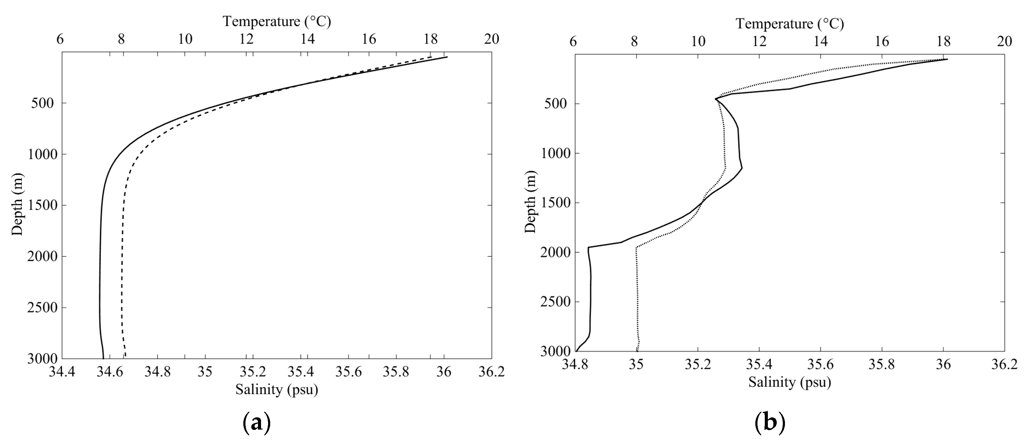
The first experiment was performed using the fully turbulent mixing model with —the nominal Munk [9] diffusivity—and the target value for vertical velocity was . The vertical T-S profiles at the center of the model domain after 200 years of integration are shown in Figure 12a. As expected for the turbulent model, which offers no constraints on the magnitude of diapycnal velocity, stratification takes a regular exponential form. Figure 12b presents the corresponding double-diffusive simulation. In this experiment, we used the functional form (Equation (12)) for the parameterization of double-diffusion, but the amplitude was adjusted upward to match the diffusivity assumed for the turbulent experiment (Figure 12a). The outcomes of these two simulations are drastically different—the stratification in the double-diffusive simulation becomes highly irregular, with fingering regions separated by deep well-mixed convecting layers.
It is also interesting to note that values of diapycnal velocity evaluated in the double-diffusive regions remain small—at least an order of magnitude less than in the corresponding turbulent experiment (Figure 12a) and, somewhat surprisingly, significantly less than the target vertical velocity. These results underscore the robust and generic tendency of double-diffusion to constrain diapycnal velocity in various configurations.
4. Theoretical Model of Double-Diffusive Insulation
Numerical simulations (Section 3) indicate that double-diffusive insulation occurs over most of the thermocline and it is not limited to Munk’s regions characterized by vertical advective-diffusive balance. Therefore our next step represents an attempt to rationalize this phenomenon without relying on the highly restrictive one-dimensional assumption used in Section 2. Over much of the main thermocline, small-scale mixing constitutes a numerically small component of the full advective-diffusive balance of temperature and salinity. Yet, this component is responsible for the diabatic water-mass transformation and, ultimately, for the selection of diapycnal velocity. Diabatic dynamics can be brought to the fore and analyzed theoretically using a procedure analogous to the one used by Rhines and Young [20], albeit in a very different context.
Consider a zero-order steady state of the ocean in the absence of mixing. This state is characterized by exact conservation of temperature, salinity, density and potential vorticity. This ideal basic state is slightly perturbed by including weak diapycnal fluxes of heat and salt in the advection-diffusion equations of motion. It is assumed that the perturbation results in only slight (first order) modification of the corresponding ideal zero order solution. The perturbed state is governed by
where and is given in Equation (23). Figure 13 represents the typical circulation pattern in the subtropical ocean on an arbitrarily chosen isopycnal surface . On this surface, we select a closed temperature contour (). Since temperature, salinity and density are assumed to be uniquely related through the linear equation of state, it follows that salinity is also constant along the chosen contours (). These contours closely follow the corresponding streamlines of the ideal basic state on which are conserved exactly.
The following analysis is pivoted about the time integrals of Equation (28) along such closed contours:
The major simplification here is achieved by elimination of the zero order advective terms. Combining Equation (29) with the double-diffusive parameterization (Equation (8)), we arrive at
The next step is the change of the integration variable from time (t) to the length coordinate measured along the contours (l), which reduces Equation (30) to
where is the absolute value of horizontal velocity. The mid-latitude circulation patterns (e.g., Figure 12) consist of two distinct regions: relatively slow geostrophic interior () and swift western boundary currents (). The inspection of Equation (31) indicates that even if a streamline passes through both regions (Figure 13), the dominant contribution to Equation (31) comes from the interior geostrophic region, where is much less (by a factor ) than the velocity in the boundary current. Neglecting the small contribution from the region of western intensification allows us to focus exclusively on geostrophic dynamics and express the horizontal velocity components as follows:
where M is the Montgomery potential. This system (Equation (32)) indicates that the contours of integration in Equation (31) at the leading order coincide with the isopleths of M. Another simplification brought by geostrophic approximation is that the Ertel potential vorticity in this case takes a relatively simple form
where C is any conservative tracer. Recall that the perturbed solution is assumed to be only slightly different from its adiabatic counterpart, which conserves temperature, salinity, and potential vorticity in the Lagrangian sense. Thus, we conclude that at the leading order (i) potential vorticity q is conserved along the contours of integration and (ii) the tracer C can be represented by any combination of temperature and salinity. Given the structure of the line integral (Equation (31)), we expect significant simplifications to occur for
Since potential vorticity is approximately uniform along each streamline, we divide Equation (31) by q, entering it directly into the integrand, which reduces the line integral to
Here, the notation “int” is used to emphasize that the integration is carried out only over the geostrophic interior. By virtue of Equation (32), we further simplify Equation (35) to
The final step is the transition from the line integrals to the area integrals over the regions bounded by closed contours of the Montgomery potential ():
Equation (37) shows that there could be no net diapycnal transport across broad regions on the isopycnal surfaces laterally bounded by closed streamlines, which confirms and rationalizes the double-diffusive insulation effect discussed and numerically modeled in Section 3. The foregoing arguments are certainly not relevant for the turbulent ocean. In the turbulent case, the flux laws do not satisfy Equation (8) and therefore Equation (30)—and all that follows—does not apply. Hence, no analogous constraints on diapycnal velocity are expected to arise in purely turbulent systems.
5. Discussion
This communication draws attention to the dramatic differences in the dynamics of diapycnal transport realized when the dominant mixing agent is double-diffusion and when mixing is controlled by mechanically-generated turbulence. Double-diffusion occurs in numerous geophysical and astrophysical fluid systems. In the ocean, nearly half of water masses are potentially affected by double-diffusive mixing [42]. Double-diffusion is also likely to play a major role in the dynamics of massive stars and giant planets [43,44]. Unlike mechanically-generated turbulence, double-diffusion is characterized by unequal eddy diffusivities of density components, which depend on the background density ratio. This feature is ultimately responsible for rather unique properties of double-diffusive mixing, such as its ability to actively constrain diapycnal volume transport—all smooth steady solutions of the T-S advection-diffusion equations are necessarily characterized by low diapycnal velocities. This property is contrasted with the passive behavior of systems dominated by mechanically generated turbulence, where it is possible to construct consistent steady-state solutions for an arbitrarily wide range of diapycnal velocities.
Our interest in the problem of diapycnal volume transport was ignited by the need to fully understand dynamics of the oceanic thermohaline circulation and associated meridional overturning. The classical view [9] ascribes small-scale diapycnal mixing a critical role for its establishment and maintenance. This notion has profoundly affected the evolution of physical oceanography. It motivated development of the extensive small-scale mixing research program, largely aimed at quantification of the average diapycnal diffusivity in the ocean [16,45]. It is commonly assumed that the increase in diapycnal diffusion of temperature and salinity necessarily amplifies the diabatic component of the meridional overturning [46]. Our study presents a peculiar counter-example of this tendency by showing that mixing can have an adverse impact on overturning. Using a suite of basin-scale simulations and theoretical models, we demonstrate that the inclusion of double-diffusion can place rather severe constraints on the magnitude of vertical diapycnal velocity. In the extreme case when vertical mixing is dominated by double-diffusion, typical values of diapycnal velocity () are less, by at least an order of magnitude, than driven by mechanically-generated turbulence with comparable T-S diffusivities. Simulations indicate that these constraints are realized both locally and in the isopycnal-average sense. In essence, double-diffusion acts to seal the thermocline by preventing the leakage of seawater (both upward and downward) across the isopycnal surfaces on which double-diffusion is a dominant mixing process. Mechanically generated turbulence, on the other hand, offers no restrictions on diapycnal velocity. When both double-diffusion and turbulence are present, the constraints on loosen (tighten) with the increase (decrease) of the fraction of the overall mixing attributed to turbulence.
When the contributions to mixing from double-diffusion and turbulence are comparable—the regime which is perhaps realized in the central Atlantic thermocline [32]—the maximum diapycnal velocity is on the order of . This value is comparable to current estimates of diapycnal velocity, which raises an intriguing possibility that diapycnal transport could be controlled by constraints on imposed by double-diffusion. This suggestion is distinct from the ideas expressed by mainstream models of thermohaline circulation [47] in which the T-S advective-diffusive dynamics constitute only a part of the problem. Ultimately, diapycnal velocity is selected by invoking three-dimensional large-scale balances involving both momentum and density. It should be realized, however, that the latter proposition is based on mixing models with uniform and equal vertical diffusivity . The examples in this paper indicate that such models may not capture all the relevant dynamics and therefore we urge caution in conceptualizing the thermohaline circulation based on oversimplified mixing parameterizations.
Our attempts to force the double-diffusive thermocline by applying a large vertical velocity which lies outside of the permitted range—the range in which smooth regular solutions can be found—have led to rather dramatic transformations of the stratification into a series well-defined convective layers separated by stratified interfaces. In this regard, it should be noted that one of the most interesting and controversial problems of double-diffusive theory concerns the origin and dynamics of so-called thermohaline staircases—stepped structures in the vertical temperature and salinity profiles. Several hypotheses have been proposed to explain the formation mechanisms [39,48] and our analysis of the “forced” experiments (Section 3.5) may add another candidate to the list. Thermohaline staircases could form as a response to strong externally imposed vertical advection, provided that the magnitude of vertical velocity is such that the advective-diffusive balance of Munk’s [9] type can only be satisfied by discontinuous step-like solutions.
Of course, there are a number of uncertainties in the presented model, particularly with regard to its ability to incorporate all relevant dynamics of the oceanic circulation. For instance, it is not clear how resilient the double-diffusive insulating blanket is in the presence of active mesoscale variability, which can also impact diapycnal transport [38]. The processes discussed in this study could be affected by the nonlinearities of the equation of state [49]. Thus, the quantitative accuracy of double-diffusive insulation theory is readily questioned. However, the differences in the way double-diffusion and turbulence affect diapycnal transport identified here are suggestive and are likely to be realized in Nature. In this regard, it should be emphasized that large-scale modeling studies which take into account double-diffusion [26,27,50] report systematic reduction in the strength of meridional overturning. Although the extent of this reduction varies considerably between models, it is possible that these results can be attributed to the double-diffusive insulation effect. Finally, it should be mentioned that while the specific solutions in this paper are based on the assumed parameterizations of double-diffusive fluxes, which require further refinements and testing, additional experiments (not shown) indicate that our results are not particularly sensitive to the choice of the functional relations for and . Therefore, we expect our qualitative conclusions to be sufficiently robust.
Acknowledgments
Support of the National Science Foundation (Grant OCE 1334914) is gratefully acknowledged.
Author Contributions
T.R. and E.E. conceived and designed the experiments; T.R. and E.E. performed the experiments; T.R. and E.E. analyzed the data; T.R. and E.E. wrote the paper.
Conflicts of Interest
The authors declare no conflict of interest.
Appendix A
Appendix A.1. Asymptotic Solutions for the Double-Diffusive Model with Weak Variation in the Flux Ratio
The one-dimensional advection-diffusion Equation (2) are non-dimensionalized using as the unit of length and as the unit of velocity. The expansion/contraction coefficients of the linear equation of state are incorporated in , and is used as the scale for both temperature and salinity. The non-dimensionalization is implemented as follows:
The governing Equation (2) and boundary conditions (Equation (3)) in non-dimensional units reduce to:
The purpose of the following theory is to examine solutions of Equation (39) in the regime where the heat/salt buoyancy flux ratio is nearly uniform. This assumption is generally supported by numerical, theoretical and experimental evidence (see the discussion in [41]). The variation in the flux ratio is fairly gentle, which makes it tempting to approximate by a constant in theoretical models [30,32]. However, this approximation, while simplifying the analytical development, also filters out some key processes affecting the dynamics of double-diffusive fluids [15,38,47]. Therefore, a more physical and precise model of the flux ratio incorporates weak variability which is determined by the density ratio: .
Appendix A.2. General Solutions
In order to extend the double-diffusive constant flux ratio model in Section 2, we consider the case when the variation in flux ratio is small but non-zero:
where . As is common in weakly nonlinear models [51], we search for a solution of the governing Equation (39) using the power series in :
These power series are substituted in the governing Equation (39) and the terms of the same order in are collected. At the zero order, we essentially arrive at the constant flux ratio model discussed in Section 2.2, which requires zero diapycnal velocity. The zero order equations for and are satisfied by the linear gradients:
The boundary conditions for the individual T-S components become:
The first order equations are given by
Multiplying the second equation by and subtracting from the first yields:
and integrating Equation (44) twice in z, subject to Equation (45) and the boundary conditions (Equation (43)), we arrive at:
Using Equations (45) and (46), we write down the second order equations:
Multiplying the second equation in Equation (47) by and subtracting from the first one yields:
The third order T-S equations are obtained in a similar manner. When the third order salinity equation is multiplied by and subtracted from the third order temperature equation, we obtain:
which is solved for using the boundary conditions (Equation (43)):
Combining Equation (50) with Equation (46), we obtain an explicit expression for :
The expansion can be similarly extended to higher orders. The significance of the foregoing analysis lies in the suggestion that similarity solutions exist in the asymptotic sector
where .
Appendix A.3. Specific Solutions
To illustrate the structure of the asymptotic solution and examine its accuracy, we now consider specific patterns of and in Equations (12) and (13). The flux ratio is taken as
which conforms to the assumed asymptotic pattern (Equation (40)) for . The following explicit expressions are obtained for , , and . In this case,
and Equations (50) and (51) reduce to:
Further extending the asymptotic expansion, we obtain the second order
and third order T-S components:
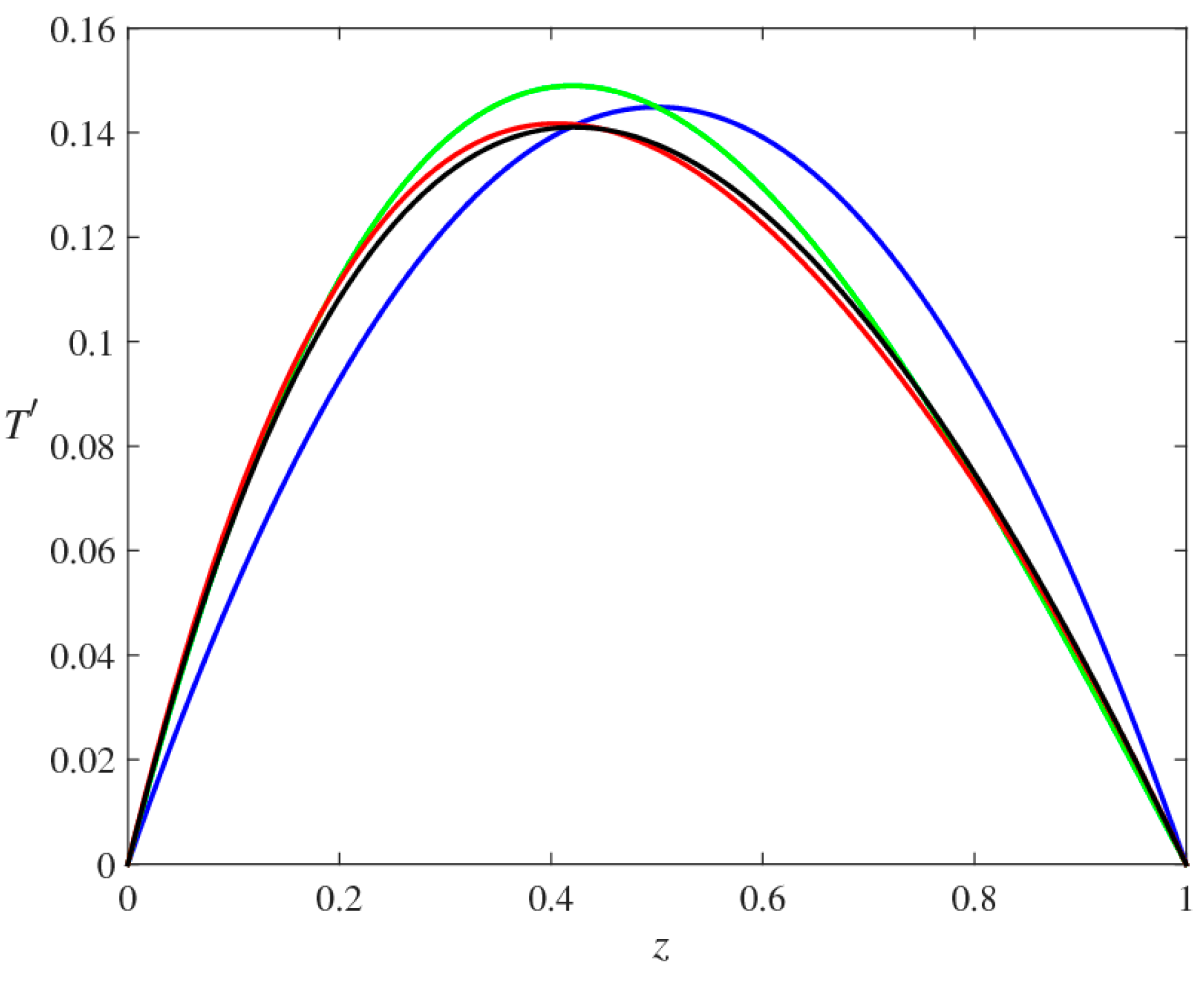
To validate the foregoing asymptotic theory, we also solve the governing equations using the numerical ODE solver of the Maple software package. A meaningful comparison of the asymptotic and numerical solutions requires some information about relevant values of , which represents the variation in the flux ratio. The pattern of the flux ratio has been studied analytically [52], numerically [24,32], experimentally [25] and observationally [7]. These studies are mutually consistent, suggesting that a reasonable choice of in the ocean would be . Therefore, in Figure A1 we present the numerical and asymptotic solutions for , (corresponding to ) and (corresponding to ). The black curve represents the numerical solution for the (non-dimensional) departure of temperature profile from the uniform gradient . The blue, green, and red curves represent the power series in that are truncated at the first, second, and third order respectively. The analytical curves rapidly converge to the numerical solution with increasing order of the expansion. The third order asymptotic closely approximates the fully nonlinear solution even for the relatively large used for the calculation in Figure A1.
Appendix A.4. Constraints on the Diapycnal Velocity
In addition to the parameters used in Figure A1, we have examined numerous other cases, all of which indicate that the asymptotic series in are remarkably accurate in describing the steady solutions of the one-dimensional advection-diffusion Equation (39) provided that such solutions exist. The question arises whether these series could be used to formulate simple explicit conditions for the existence of solutions.
If , then all coefficients of the power series in for T and S are of order one. Such series are generally characterized by a finite radius of convergence. This implies that for , solutions always exist as long as is sufficiently small. What happens when ? In this case, the asymptotic series for temperature and salinity can be approximated by
where the coefficients are independent of and . These power series for are also valid only within a finite radius of convergence. Thus, denoting the radius of convergence of the series in Equation (57) by , we can expect the existence of regular solutions for T and S for as long as
When Equation (58) is rewritten in terms of and , we arrive at the explicit constraint on the diapycnal velocity:
This result is highly suggestive—Equation (59) implies that the range of diapycnal velocities is proportional to the effective variation in the flux ratio. To systematically test this prediction, we have performed a series of numerical calculations in which we varied and . The results obtained with and the flux parameterizations in Equations (12), (13) and (53) are shown in Figure A2. The dots in parameter space represent all attempts to solve the governing equations. The experiments in which regular solutions have been found are indicated by heavy dots, whereas the light dots represent conditions for which the numerical search for solutions failed. The results in Figure A2 are consistent with the theoretical prediction in Equation (59). All solutions are largely confined to two sectors—corresponding to positive and negative —bounded by straight lines emanating from the (0,0) point in the parameter space.
It is also of interest to examine the relevant range of diapycnal velocities in the double-diffusive zone in Figure A2. Assuming that the variation of flux ratio in the ocean is , we obtain non-dimensional constraint . This estimate can be expressed in terms of dimensional variables by reverting the non-dimensionalization Equation (38). For and , we obtain the maximum dimensional diapycnal velocity of
This estimate suggests that double-diffusion could severely constrain the diapycnal velocity. To interpret Equation (60) in the global circulation context, let us recall that the nominal value of diapycnal velocity, commonly used in climate models [42], is , exceeding Equation (60) by more than an order of magnitude. Thus, the diapycnal transport, both upward and downward, can be essentially blocked in the ocean regions where mixing is dominated by double-diffusion. Finally, we note that Equation (60) was obtained on the basis of one-dimensional arguments. Nevertheless, the range of diapycnal velocities realized in three-dimensional double-diffusive simulations (Section 3) is of the same order as Equation (60) and much less than in the corresponding turbulent experiments (e.g., Figure 7 and Figure 8).
Figure A1.
The non-dimensional departure of temperature from the linear gradient . is computed numerically (black curve) and compared with the calculation based on the asymptotic expansion in truncated at the first, second, and third orders (blue, green, and red curves respectively). For (), the numerical result is almost indistinguishable from the third order asymptotic prediction.

Figure A2.
The range of diapycnal velocities permitted in the one-dimensional model with variable flux ratio (). Parameter measures the extent of variation in , with positive (negative) values corresponding to the increasing (decreasing) relation. The numerical calculations resulting in regular solutions are indicated by heavy dots and light dots represent conditions under which no solutions were found.

References
- Mirouh, G.M.; Garaud, P.; Stellmach, S.; Traxler, A.L.; Wood, T.S. A new model for mixing by double-diffusive convection (semi-convection). I. The conditions for layer formation. Astrophys. J. 2012, 750, 61. [Google Scholar] [CrossRef]
- Brown, J.M.; Garaud, P.; Stellmach, S. Chemical transport and spontaneous layer formation in fingering convection in astrophysics. Astrophys. J. 2013, 768, 34. [Google Scholar] [CrossRef]
- Radko, T.; Smith, D.P. Equilibrium transport in double-diffusive convection. J. Fluid Mech. 2012, 692, 5–27. [Google Scholar] [CrossRef] [Green Version]
- McDougall, T.J. The relative roles of diapycnal and isopycnal mixing on subsurface water mass conversion. J. Phys. Oceanogr. 1984, 14, 1577–1589. [Google Scholar] [CrossRef]
- McDougall, T.J. Thermobaricity, cabbeling, and water-mass conversion. J. Geophys. Res. 1987, 92, 5448–5464. [Google Scholar] [CrossRef]
- McDougall, T.J.; Ruddick, B.R. The use of ocean microstructure to quantify both turbulent mixing and salt-fingering. Deep Sea Res. 1992, 39, 1931–1952. [Google Scholar] [CrossRef]
- St. Laurent, L.; Toole, J.M.; Schmitt, R.W. Buoyancy forcing by turbulence above rough topography in the abyssal Brazil basin. J. Phys. Oceanogr. 2001, 31, 3476–3495. [Google Scholar] [CrossRef]
- Robinson, A.R.; Stommel, H. The oceanic thermocline and the associated thermohaline circulation. Tellus 1959, 11, 295–308. [Google Scholar]
- Munk, W. Abyssal recipes. Deep Sea Res. 1966, 13, 707–730. [Google Scholar] [CrossRef]
- Welander, P. Thermohaline effects in the ocean circulation and related simple models. In Large-Scale Transport Processes in Oceans and Atmosphere; Willebrand, J., Anderson, D.L.T., Eds.; Springer Netherland: Dordrecht, The Netherlands, 1986; pp. 163–200. [Google Scholar]
- Whitehead, J.A. Thermohaline ocean processes and models. Annu. Rev. Fluid Mech. 1995, 27, 89–113. [Google Scholar] [CrossRef]
- Toggweiler, J.R.; Samuels, B. On the ocean’s large-scale circulation near the limit of no vertical mixing. J. Phys. Oceanogr. 1998, 28, 1832–1852. [Google Scholar] [CrossRef]
- Gnanadesikan, A. A simple predictive model for the structure of the oceanic pycnocline. Science 1999, 283, 2077–2079. [Google Scholar] [CrossRef] [PubMed]
- Radko, T.; Kamenkovich, I. Semi-adiabatic model of the deep stratification and meridional overturning. J. Phys. Oceanogr. 2011, 41, 757–780. [Google Scholar] [CrossRef]
- Radko, T.; Kamenkovich, I.; Dare, P. Inferring the pattern of the oceanic meridional transport from the air-sea density flux. J. Phys. Oceanogr. 2008, 38, 2722–2738. [Google Scholar] [CrossRef]
- Munk, W.; Wunsch, C. Abyssal recipes II: Energetics of tidal and wind mixing. Deep Sea Res. 1998, 45, 1977–2010. [Google Scholar] [CrossRef]
- Boccaletti, G.; Ferrari, R.; Adcroft, A.; Ferreira, D.; Marsh, J. The vertical structure of ocean heat transport. Geophys. Res. Lett. 2005, 32, 10. [Google Scholar] [CrossRef]
- Schmitt, R.W. Double diffusion in oceanography. Annu. Rev. Fluid Mech. 1994, 26, 255–285. [Google Scholar] [CrossRef]
- Luyten, J.R.; Pedlosky, J.; Stommel, H. The ventilated thermocline. J. Phys. Oceanogr. 1983, 13, 292–309. [Google Scholar] [CrossRef]
- Rhines, P.B.; Young, W.R. A theory of the wind-driven circulation. I. Mid-ocean gyres. J. Mar. Res. 1982, 40, 559–596. [Google Scholar]
- Merryfield, W.J.; Holloway, G.; Gargett, A.E. Differential vertical transport of heat and salt by weak stratified turbulence. Geophys. Res. Lett. 1998, 25, 2773–2776. [Google Scholar] [CrossRef]
- Gargett, A.E. Differential diffusion: An oceanographic primer. Proress. Oceanogr. 2003, 56, 559–570. [Google Scholar] [CrossRef]
- Schmitt, R.W. Observational and laboratory insights into salt finger convection. Prog. Oceanogr. 2003, 56, 419–433. [Google Scholar] [CrossRef]
- Radko, T. Double-Diffusive Convection; Cambridge University Press: New York, NY, USA, 2013; p. 344. [Google Scholar]
- Schmitt, R.W. Form of the temperamre-salinity relationship in the Central Water: Evidence for double-diffusive mixing. J. Phys. Oceanogr. 1981, 11, 1015–1026. [Google Scholar] [CrossRef]
- Zhang, J.; Schmitt, R.W.; Huang, R.X. Sensitivity of GFDL Modular Ocean Model to the parameterization of double-diffusive processes. J. Phys. Oceanogr. 1998, 28, 589–605. [Google Scholar] [CrossRef]
- Merryfield, W.J.; Holloway, G.; Gargett, A.E. A global ocean model with double-diffusive mixing. J. Phys. Oceanogr. 1999, 29, 1124–1142. [Google Scholar] [CrossRef]
- Wells, M.G.; Griffiths, R.W. Interaction of salt finger convection with intermittent turbulence. J. Geophys. Res. 2003, 108. [Google Scholar] [CrossRef]
- Smyth, W.D.; Kimura, S. Mixing in a moderately sheared salt-fingering layer. J. Phys. Oceanogr. 2011, 41, 1364–1384. [Google Scholar] [CrossRef]
- Schmitt, R.W.; Perkins, H.; Boyd, J.D.; Stalcup, M.C. C-SALT: An investigation of the thermohaline staircase in the western tropical North Atlantic. Deep Sea Res. 1987, 34, 1697–1704. [Google Scholar] [CrossRef]
- Schmitt, R.W.; Ledwell, J.R.; Montgomery, E.T.; Polzin, K.L.; Toole, J.M. Enhanced diapycnal mixing by salt fingers in the thermocline of the tropical Atlantic. Science 2005, 308, 685–688. [Google Scholar] [CrossRef] [PubMed]
- St. Laurent, L.; Schmitt, R.W. The contribution of salt fingers to vertical mixing in the North Atlantic tracer release experiment. J. Phys. Oceanogr. 1999, 29, 1404–1424. [Google Scholar] [CrossRef]
- Marshall, J.; Adcroft, A.; Hill, C.; Perelman, L.; Heisey, C. A finite-volume, incompressible Navier Stokes model for studies of the ocean on parallel computers. J. Geophys. Res. 1997, 102, 5753–5766. [Google Scholar] [CrossRef]
- Marshall, J.; Hill, C.; Perelman, L.; Adcroft, A. Hydrostatic, quasi-hydrostatic, and nonhydrostatic ocean modeling. J. Geophys. Res. 1997, 102, 5733–5752. [Google Scholar] [CrossRef]
- Large, W.G.; McWilliams, J.C.; Doney, S.C. Oceanic vertical mixing: A review and a model with a nonlocal boundary layer parameterization. Rev. Geophys. 1994, 32, 363–403. [Google Scholar] [CrossRef]
- Gent, P.; McWilliams, J. Isopycnal mixing in ocean circulation models. J. Phys. Oceanogr. 1990, 20, 150–155. [Google Scholar] [CrossRef]
- Pedlosky, J. Geophysical Fluid Dynamics; Springer: Berlin, Germany, 1987; p. 710. [Google Scholar]
- Radko, T.; Marshall, J. Eddy-induced diapycnal fluxes and their role in the maintenance of the thermocline. J. Phys. Oceanogr. 2004, 34, 372–383. [Google Scholar] [CrossRef]
- Radko, T. A mechanism for layer formation in a double-diffusive fluid. J. Fluid Mech. 2003, 497, 365–380. [Google Scholar] [CrossRef]
- Stellmach, S.; Traxler, A.; Garaud, P.; Brummell, N.; Radko, T. Dynamics of fingering convection II: The formation of thermohaline staircases. J. Fluid Mech. 2011, 677, 554–571. [Google Scholar] [CrossRef] [Green Version]
- Radko, T.; Bulters, A.; Flanagan, J.; Campin, J.M. Double-diffusive recipes. Part I: Large-scale dynamics of thermohaline staircases. J. Phys. Oceanogr. 2014, 44, 1269–1284. [Google Scholar] [CrossRef]
- You, Y. A global ocean climatological atlas of the Turner angle: Implications for double-diffusion and water mass structure. Deep Sea Res. 2002, 49, 2075–2093. [Google Scholar] [CrossRef]
- Merryfield, W.J. Hydrodynamics of semiconvection. Astrophys. J. 1995, 444, 318–337. [Google Scholar] [CrossRef]
- Garaud, P. What happened to the other mohicans? The case for a primordial origin to the planet-metallicity connection. Astrophys. J. Lett. 2011, 728, L30. [Google Scholar] [CrossRef]
- Wunsch, C.; Ferrari, R. Vertical mixing, energy, and the general circulation of the oceans. Ann. Rev. Fluid Mech. 2004, 36, 281–314. [Google Scholar] [CrossRef]
- Bryan, F. Parameter sensitivity of primitive equation ocean general circulation models. J. Phys. Oceanogr. 1987, 17, 970–985. [Google Scholar] [CrossRef]
- Welander, P. The thermocline problem. Philos. Trans. R. Soc. Lond. 1971, 270, 69–73. [Google Scholar] [CrossRef]
- Merryfield, W.J. Origin of thermohaline staircases. J. Phys. Oceanogr. 2000, 30, 1046–1068. [Google Scholar] [CrossRef]
- Ozgokmen, T.M.; Esenkov, O.E. Asymmetric salt fingers induced by a nonlinear equation of state. Phys. Fluids 1998, 10, 1882–1890. [Google Scholar] [CrossRef]
- Gargett, A.E.; Holloway, G. Sensitivity of the GFDL ocean model to different diffusitivities for heat and salt. J. Phys. Oceanogr. 1992, 22, 1158–1177. [Google Scholar] [CrossRef]
- Malkus, W.V.R.; Veronis, G. Finite amplitude cellular convection. J. Fluid Mech. 1958, 4, 225–260. [Google Scholar] [CrossRef]
- Schmitt, R.W. The growth rate of supercritical salt fingers. Deep Sea Res. 1979, 26, 23–44. [Google Scholar] [CrossRef]
Figure 1.
One-dimensional model. We search for the temperature and salinity profiles and satisfying the vertical advection-diffusion equations for given vertical velocity () and boundary conditions at the ends of the mixing zone ().
Figure 1.
One-dimensional model. We search for the temperature and salinity profiles and satisfying the vertical advection-diffusion equations for given vertical velocity () and boundary conditions at the ends of the mixing zone ().

Figure 2.
The range of diapycnal velocities permitted in the hybrid model which includes both double-diffusive and turbulent mixing. Parameter measures the relative contributions from turbulence and double-diffusion to the net mixing. The numerical calculations resulting in regular solutions are indicated by heavy dots and light dots represent conditions under which no solutions were found.

Figure 3.
The meridional patterns of the model forcing fields. Thermohaline forcing is applied by relaxing the surface temperature and salinity to the target patterns shown in (a) and (b) respectively. The wind stress is shown in (c). All forcing fields are zonally-uniform.
Figure 3.
The meridional patterns of the model forcing fields. Thermohaline forcing is applied by relaxing the surface temperature and salinity to the target patterns shown in (a) and (b) respectively. The wind stress is shown in (c). All forcing fields are zonally-uniform.

Figure 4.
The final state () realized in the numerical experiments with double-diffusive mixing (the constant flux ratio case): (a) The horizontal temperature distribution and velocity pattern at ; (b) The zonal section of temperature at . Clearly visible is a well-defined thermocline with relatively warm water extending several hundred meters downward from the surface.

Figure 5.
Three-dimensional view of the average isopycnal surface defined in Equation (19). Color coding represents the density ratio distribution on this isopycnal. The observed range of density ratios indicates that fingering is active and that its intensity is relatively high.
Figure 5.
Three-dimensional view of the average isopycnal surface defined in Equation (19). Color coding represents the density ratio distribution on this isopycnal. The observed range of density ratios indicates that fingering is active and that its intensity is relatively high.

Figure 6.
Physical interpretation of diapycnal velocity. A Lagrangian particle initially located on a motionless tilted isopycnal surface is advected from A to B by a cross-isopycnal flow. Point C is the vertical projection of B onto the isopycnal surface. Diapycnal velocity represents the rate of the increase in vertical separation of the Lagrangian point from the isopycnal surface.

Figure 7.
Diapycnal transport in the double-diffusive and turbulent oceans. Diapycnal velocity is evaluated at the average isopycnal surface in the ocean interior () and shown for the double-diffusive (a) and turbulent (b) experiments. In the double-diffusive case, typical values of are on the order of or less with both positive and negative values observed. In the turbulent experiment, diapycnal velocities are mostly positive and larger by at least an order of magnitude ().

Figure 8.
The vertical distribution of diapycnal transport. (a) The mean diapycnal velocity evaluated at various isopycnals () and plotted as a function of the average depth of those surfaces; (b) The local vertical profile of diapycnal velocity () at . Both diagnostics indicate that diapycnal velocity in the turbulent case (indicated by the blue curves) substantially exceeds that in the double-diffusive ocean (green curves). The patterns of and are qualitatively similar.

Figure 9.
The variation of the mean diapycnal velocity at the density surface () as a function of . The diagnostics are based on a series of simulations which incorporate both double-diffusive and turbulent mixing. Note the monotonic increase in with increasing .
Figure 9.
The variation of the mean diapycnal velocity at the density surface () as a function of . The diagnostics are based on a series of simulations which incorporate both double-diffusive and turbulent mixing. Note the monotonic increase in with increasing .

Figure 10.
The assumed patterns of the flux ratio (a) and salt diffusivity (b) used for parameterization of double-diffusion in the numerical simulations (Section 3.4).
Figure 10.
The assumed patterns of the flux ratio (a) and salt diffusivity (b) used for parameterization of double-diffusion in the numerical simulations (Section 3.4).

Figure 11.
A series of large-scale simulations in which the variation in the flux ratio (as measured by the parameter ) is systematically increased. For each experiment, the mean diapycnal velocity () at the average isopycnal surface is plotted as a function of . Note the monotonic—nearly linear—increase in with .

Figure 12.
Vertical T-S profiles obtained with the “forced” model, in which upward vertical velocity was prescribed below the surface and above the sea-floor of the model ocean. The solid (dashed) curves represent the salinity (temperature) profiles: (a) The experiment in which vertical mixing is represented by turbulent diffusion with uniform and equal T-S diffusivities; (b) The analogous experiment performed with double-diffusive mixing. Note the dramatic differences in the resulting stratification patterns.

Figure 13.
Schematic diagram illustrating the analytical model of double-diffusive insulation. The model suggests that the average diapycnal velocity in the regions bounded by closed streamlines on the density surfaces in the ocean interior (indicated by grey shading) is zero if vertical mixing is double-diffusive but can be finite in the presence of mechanically generated turbulence.

© 2016 by the authors; licensee MDPI, Basel, Switzerland. This article is an open access article distributed under the terms and conditions of the Creative Commons Attribution license ( http://creativecommons.org/licenses/by/4.0/).
Share and Cite
MDPI and ACS Style
Radko, T.; Edwards, E. Diapycnal Velocity in the Double-Diffusive Thermocline. Fluids 2016, 1, 25. https://doi.org/10.3390/fluids1030025
AMA Style
Radko T, Edwards E. Diapycnal Velocity in the Double-Diffusive Thermocline. Fluids. 2016; 1(3):25. https://doi.org/10.3390/fluids1030025
Chicago/Turabian StyleRadko, Timour, and Erick Edwards. 2016. "Diapycnal Velocity in the Double-Diffusive Thermocline" Fluids 1, no. 3: 25. https://doi.org/10.3390/fluids1030025