Estimating Eulerian Energy Spectra from Drifters

Abstract

The relations between the kinetic energy spectrum and the second-order longitudinal structure function for 2D non-divergent flow are derived, and several examples are considered. The transform from spectrum to structure function is illustrated using idealized power-law spectra of turbulent inertial ranges. The results illustrate how the structure function integrates contributions across wavenumber, which can obscure the dependencies when the inertial ranges are of finite extent. The transform is also applied to the kinetic energy spectrum of Nastrom and Gage (1985), derived from aircraft data in the upper troposphere; the resulting structure function agrees well with that of Lindborg (1999), calculated with the same data. The transform from structure function to spectrum is then tested with data from 2D turbulence simulations. When applied to the (Eulerian) structure function obtained from the transform of the spectrum, the result closely resembles the original spectrum, except at the largest wavenumbers. The deviation at large wavenumbers occurs because the transform involves a filter function which magnifies contributions from large separations. The results are noticeably worse when applied to the structure function obtained from pairs of particles in the flow, as this is usually noisy at large separations. Fitting the structure function to a polynomial improves the resulting spectrum, but not sufficiently to distinguish the correct inertial range dependencies. Furthermore, the transform of steep (non-local) spectra is largely unsuccessful. Thus, it appears that with Lagrangian data, it is probably preferable to focus on structure functions, despite their shortcomings.

1. Introduction

Large-scale turbulence in the ocean is responsible for the fluxes of energy, enstrophy and tracers across scales. Turbulence, for example, facilitates the dissipation of energy injected by the winds [1]. However, the exact nature of the turbulence remains uncertain because it is difficult to quantify kinetic energy spectra in the ocean. Satellite data, which has the spatial coverage required for such quantification, is limited in horizontal resolution, which is of order of 100 km [2,3]. Shipboard current measurements can produce finer resolution estimates, down to several kilometers, in targeted regions [4,5]. However, there are still relatively few studies in which spectra have been calculated, and the results often differ with region.

The present work concerns using Lagrangian data—specifically, the trajectories of pairs of drifting buoys—to estimate Eulerian energy spectra. There is currently a wealth of Lagrangian data, both at the surface and below the surface, with global coverage. The newest generation of surface drifters in particular are tracked via the Global Positioning System (GPS), yielding positions with 10 m accuracy. Thus, Lagrangian data offers the tantalizing possibility of measuring energy spectra down to such scales, in most parts of the global ocean.

The study of particle pair or “relative” dispersion dates back to Richardson [6], who studied the spreading of smoke from factory stacks . It was recognized subsequently that pair dispersion in turbulent flows depends on the kinetic energy spectrum, and Richardson’s observations were shown to be consistent with a Kolmogorov energy spectrum [7]. Thus, relative dispersion offers a means for deducing kinetic energy spectra in turbulent flows.

A number of studies have examined the connection between relative dispersion and turbulence spectra [8,9,10,11,12]. “Local dispersion” occurs when pairs are influenced by eddies with scales comparable to the pair separation and “non-local dispersion” when they are dominated by larger eddies. Under local dispersion, the mean square pair separation (the dispersion) exhibits power-law growth, with an exponent related to the slope of the energy spectrum [9]. Under non-local dispersion, the dispersion grows exponentially in time.

In the atmosphere, exponential dispersion was observed at separations below 2000 km in balloon experiments [13,14]. Exponential dispersion has also been observed at the ocean surface, at scales below the Rossby radius of deformation [15,16,17]. The balloon- and drifter-derived results agree with independent Eulerian estimates at these scales in the atmosphere [18] and ocean [4]. However, different conclusions have also been made. The aforementioned balloon dispersion is possibly also consistent with local dispersion [19], and there is evidence for local dispersion in the ocean as well, both at the surface [20,21] and subsurface [22,23].

In all such cases though, the energy spectra were inferred from dispersion. However, under certain conditions the energy spectra can be calculated directly from velocity differences from pairs of drifters. The following focuses on this calculation in 2D flows, which are appropriate for large-scale motion in the atmosphere and ocean. We examine the results in different applications, including atmospheric spectra and 2D turbulence simulations.

2. Spectra and Structure Functions

In a homogeneous flow, the two-point velocity autocorrelation and the kinetic energy spectrum are related via the Fourier transform [24]:

$$R_{ij}\left(\overrightarrow{r}\right)={\int }_{-\infty }^{\infty }{\int }_{-\infty }^{\infty }{\mathsf{\Phi }}_{ij}(k,l)e^{i\overrightarrow{k}·\overrightarrow{r}}dkdl,{\mathsf{\Phi }}_{ij}(k,l)=\frac{1}{{\left(2\pi \right)}^2}{\int }_{-\infty }^{\infty }{\int }_{-\infty }^{\infty }{R}_{ij}\left(\overrightarrow{r}\right)e^{-i\overrightarrow{k}·\overrightarrow{r}}d{r}_{x}d{r}_y,$$

(1)

where:

$$R_{ij}\equiv <u_i(\overrightarrow{x}+\overrightarrow{r})u_j\left(\overrightarrow{x}\right)>.$$

The brackets indicate an ensemble average; assuming ergodicity, this is calculated as an area average over $\overrightarrow{x}$. Similar relations apply in three dimensions as well, but we will focus on two dimensions hereafter. For an isotropic flow, the spectrum depends only on the magnitude of the wavenumber, K. Then correlation is given by:

$$R_{ij}\left(r\right)=2\pi {\int }_0^{\infty }{\mathsf{\Phi }}_{ij}\left(K\right)J_o\left(Kr\right)KdK.$$

(2)

Thus, $R_{ij}\left(r\right)$ is the Hankel transform of ${\mathsf{\Phi }}_{ij}$. The kinetic energy is just the trace of $R_{ij}$ at zero separation:

$$E_{tot}=\frac{1}{2}{R}_{ii}\left(0\right)={\int }_0^{\infty }\pi {\mathsf{\Phi }}_{ii}KdK\equiv {\int }_0^{\infty }E\left(K\right)dK,$$

(3)

with summation implied for repeated indices. The inverse relation follows from the orthogonality condition for Hankel transforms and is:

$$E\left(K\right)=\frac{1}{2}{\int }_0^{\infty }{R}_{ii}\left(r\right)Kr{J}_0\left(Kr\right)dr.$$

(4)

In homogeneous and isotropic flows, the two-point correlation can be determined from either Eulerian or Lagrangian measurements.

The velocity correlation, in turn, can be written in terms of the longitudinal (f) and transverse (g) velocity correlations [24]:

$$R_{ij}=\frac{f-g}{r^2}{r}_i{r}_j+g{\delta }_{ij},$$

(5)

where ${\delta }_{ij}$ is one for equal indices and zero otherwise, and:

$$f\left(r\right)=<u_{\parallel }(\overrightarrow{x}+\overrightarrow{r})u_{\parallel }\left(\overrightarrow{x}\right)>,g\left(r\right)=<u_{\perp }(\overrightarrow{x}+\overrightarrow{r})u_{\perp }\left(\overrightarrow{x}\right)>,$$

(6)

with parallel and perpendicular referring to the separation vector, $\overrightarrow{r}$. Relation (5) derives from symmetry conditions relevant for isotropic matrices [24].

Imposing continuity in 2D requires:

$$\frac{\partial }{\partial x_i}{R}_{ij}=0\to g=f+r\frac{\partial f}{\partial r}=\frac{\partial }{\partial r}\left(rf\right),$$

(7)

(see also [25,26,27]). (2D non-divergence is a somewhat restrictive assumption for the ocean. The geostrophic velocities are 2D non-divergent, but deviations occur at smaller scales, where the Rossby number is order one. At such scales, the flow is also less 2D, so a shift to 3D might be considered). Using (7), $R_{ii}$ can be written:

$$R_{ii}=f-g+2g=f+g=f+\frac{\partial }{\partial r}\left(rf\right).$$

(8)

Substituting this into (4):

$$E\left(K\right)=\frac{1}{2}{\int }_0^{\infty }[f+\frac{\partial }{\partial r}\left(rf\right)]Kr{J}_0\left(Kr\right)dr=\frac{1}{2}{\int }_0^{\infty }f{K}^2{r}^2{J}_1\left(Kr\right)dr,$$

(9)

after integration by parts, and assuming that f vanishes at infinity. The inverse relation is:

$$f\left(r\right)=2{\int }_0^{\infty }E\left(K\right)\frac{J_1\left(Kr\right)}{Kr}dK.$$

(10)

Thus, $E/\left(K^{2}r\right)$ and $K^{2}rf$ are also a Hankel transform pair. Expressions (9) and (10) are the 2D counterparts of Batchelor’s expressions 3.4.16 [24].

A common measure used in analyzing turbulent flows is the second-order velocity structure function [24,28]:

$$S_2\left(r\right)\equiv <{|\overrightarrow{u}(\overrightarrow{x}+\overrightarrow{r})-\overrightarrow{u}\left(\overrightarrow{x}\right)|}^2>.$$

(11)

In a homogeneous and isotropic flow, the longitudinal component, $S_{2l}\left(r\right)$, can be measured from the separation velocity of pairs of particles (e.g., [11]):

$$S_{2l}\left(r\right)=<{\left(\frac{d}{dt}{r}_{ij}\right)}^2{>|}_r,$$

(12)

where $r_{ij}$ is the magnitude of the particle separation vector. Note that $S_{2l}$ on the left side of (12) is an Eulerian measure while the average on the right side is Lagrangian. The brackets indicate that the average is conditioned by r, the magnitude of the separation.

The structure function in turn is related to the longitudinal velocity correlation:

$$S_{2l}\left(r\right)\equiv <{(u_{||}(\overrightarrow{x}+\overrightarrow{r})-u_{||}\left(\overrightarrow{x}\right))}^2>=2f\left(0\right)-2f\left(r\right)=2E_{tot}-2f\left(r\right),$$

(13)

assuming the flow is isotropic. Thus:

$$S_{2l}\left(r\right)=2{\int }_0^{\infty }E\left(K\right)(1-\frac{2J_1\left(Kr\right)}{Kr})dK.$$

(14)

Expression (14) is similar to Equation (3.1) of [9], except that the latter relates instead to the full structure function. What differs is the factor in parentheses (the full expression has $1-J_0\left(Kr\right)$). The two expressions behave similarly, however, acting as high pass filters (Figure 1). For small arguments ($Kr\ll 1$), the filter is proportional to $K^2{r}^2$ (see below), while for large arguments, it approaches one. Hence, $S_{2l}\left(r\right)$ asymptotes to twice the total kinetic energy at large separations.

The energy can be determined from the inverse relation, which follows from (9):

$$E\left(K\right)=\frac{1}{2}{\int }_0^{\infty }[E_{tot}-\frac{S_{2l}\left(r\right)}{2}]K^2{r}^2{J}_1\left(Kr\right)dr.$$

(15)

An important point here is that the filter, $K^2{r}^2{J}_1\left(Kr\right)$, has no asymptotic limit for large values of $Kr$. Even though divergence of the integral is avoided because $[E_{tot}-\frac{S_{2l}\left(r\right)}{2}]\to 0$, the filter magnifies the response at large separations. This hinders the inversion, as seen hereafter. Nevertheless, a particle-derived structure function can, in principle, be used to calculate the energy spectrum.

3. Idealized Spectra

We first examine calculating the structure function from the spectrum. Consider an idealized spectrum:

$$E\left(K\right)=E_0{\left(\frac{K}{K_o}\right)}^{-\alpha }{K}_0<K<K_1.$$

(16)

The spectrum has a finite range (rather than extending from $K=0$ to $K=\infty$) and thereby avoids associated singularities.

The dependence of the longitudinal structure function on separation can be deduced using an approximate version of the high pass filter in (14), based on the asymptotic limits of that filter:

$$HF=\left\{\begin{array}{cc}\frac{K^2{r}^2}{8}\hfill & \mathrm{if}Kr\le 2\sqrt{2}\hfill \\ 1\hfill & \mathrm{if}Kr>2\sqrt{2}.\hfill \end{array}\right.$$

(17)

This is plotted in Figure 1 (its validity as a substitute for the actual filter is demonstrated hereafter). Using (17), the structure function (14) is approximately:

$$\begin{array}{c}\hfill S_{2l}\left(r\right)\approx 2{\int }_0^{2\sqrt{2}/r}{E}_0{\left(\frac{K}{K_o}\right)}^{-\alpha }\frac{K^2{r}^2}{8}dK+2{\int }_{2\sqrt{2}/r}^{K_1}{E}_0{\left(\frac{K}{K_o}\right)}^{-\alpha }dK\\ \hfill =\frac{E_0{K}_0^{\alpha }}{4(3-\alpha )}{r}^2{K}^{3-\alpha }{{|}_{K_0}^{2\sqrt{2}/r}+\frac{2E_0{K}_0^{\alpha }}{1-\alpha }{K}^{1-\alpha }|}_{2\sqrt{2}/r}^{K_1}\end{array}$$

(18)

for inverse separations in the spectral range. If $\alpha >3$ (a non-local spectrum) and the lower wavenumber, $K_0$, is sufficiently small, the integral is approximately:

$$S_{2l}\left(r\right)\approx \frac{E_0{K}_0^3}{16{\pi }^2(\alpha -3)}{r}^2.$$

(19)

The structure function increases as $r^2$, regardless of how steep the spectrum is. If the slope is such that $1<\alpha <3$ (local spectrum) and $K_1$ is sufficiently large, the second term dominates:

$$S_{2l}\left(r\right)\approx \frac{2E_0{K}_0^{\alpha }}{(\alpha -1){\left(2\pi \right)}^{\alpha -1}}{r}^{\alpha -1}.$$

(20)

For a Kolmogorov spectrum ($\alpha =5/3$), the structure function scales as $r^{2/3}$. However, unless the spectral range is long ($K_1\gg K_0$), the other terms will contribute and cause deviations. This illustrates the difficulty with examining the structure function alone: it mixes contributions from different parts of the spectrum.

For large separations, $r\gg 1/K_0$, the structure function is constant:

$$S_{2l}\left(r\right)=2{\int }_{K_0}^{K_1}EdK=2E_{tot}.$$

(21)

Thus, the lower wavenumber limit, $K_0$, determines the scale at which $S_{2l}$ flattens out.

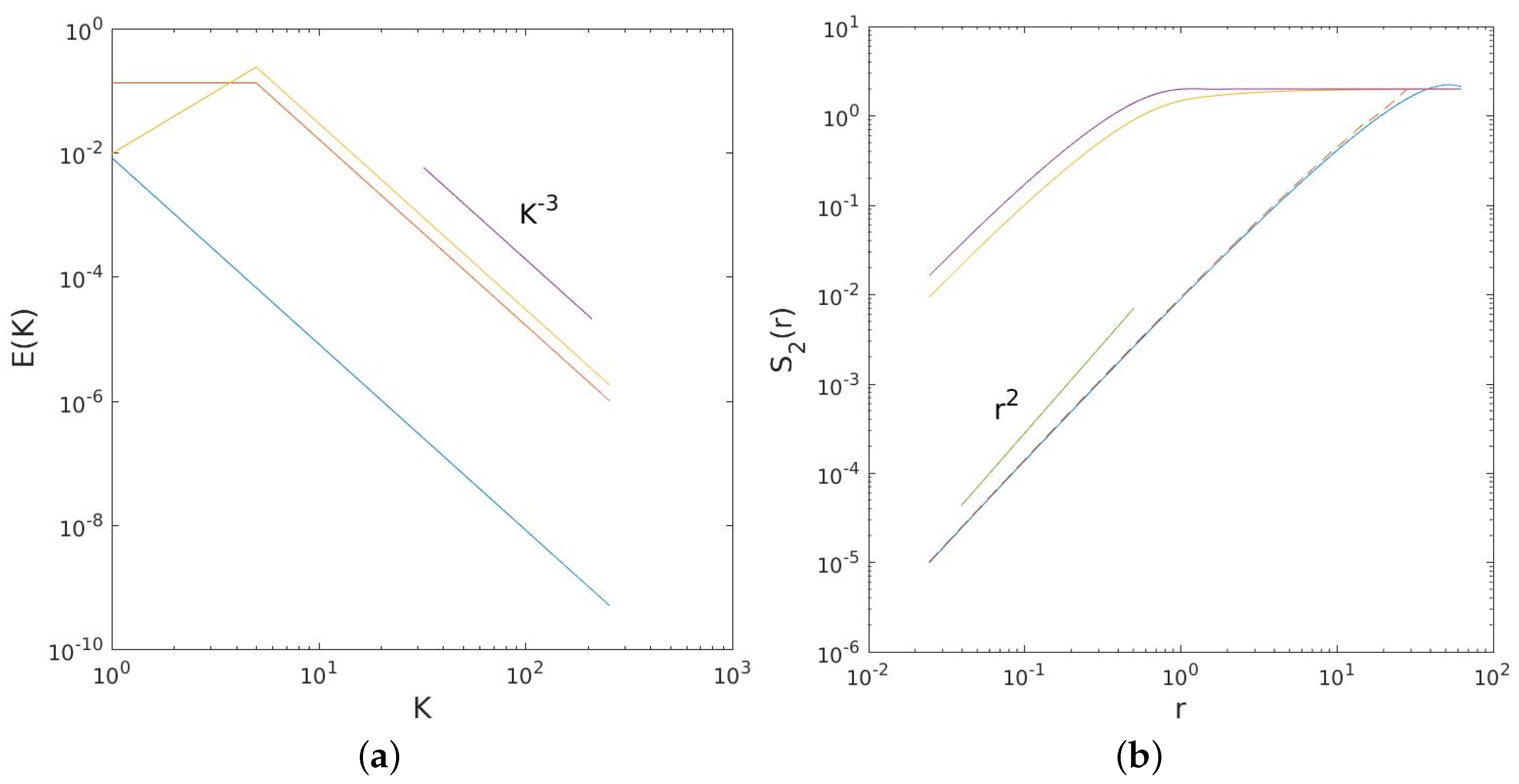
The transform with $\alpha =3$ is shown in Figure 2 (the results with local spectra are qualitatively similar). The case above is plotted in blue in the left panel, with $K_0=1$ and $K_1=256$. The two other spectra peak instead at $K=5$. The structure functions in the right panel were calculated numerically from (14).

The structure function for the spectrum peaked at $K_0$ is shown in blue in the right panel. This increases more slowly than $r^2$, illustrating the effect of having a finite wavenumber range. The two other spectra exhibit a similar increase at small scales but level off sooner, due to having a larger peak wavenumber. Note too that the difference at low wavenumbers between the two spectra with $K=5$ has little impact on the structure functions. This reflects the greater importance of the large wavenumbers in (14).

In addition, there is the dashed curve in Figure 2, the structure function obtained using the approximate filter in (17). This is nearly the same as the structure function obtained using the full filter, which supports using (18) to infer the limiting behavior. The similarity implies that the oscillations due to the Bessel function have little impact on the integrals.

4. The Nastrom and Gage (1985) Spectrum

For a more realistic example, consider a spectrum from the upper troposphere. Nastrom and Gage [18] calculated zonal and meridional wavenumber spectra using data collected from commercial aircraft over the United States. Lindborg [26] subsequently calculated longitudinal and transverse structure functions, using the same data. Lindborg rationalized the structure functions using asymptotic limits appropriate for the two inertial ranges seen in the Nastrom and Gage spectra, specifically $K^{-3}$ for separations from 2000 km to several hundred kilometers, and $K^{-5/3}$ at smaller scales.

However, one can estimate the longitudinal structure function directly from the spectra, using (14). We extracted the zonal and meridional spectra from Figure 3 of [18] (the data were obtained digitally using Engauge digitizer software (http://markummitchell.github.io/engauge-digitizer/)). Assuming the flight tracks were primarily east–west, we used the zonal spectrum to approximate the longitudinal component. We then evaluated (14), numerically.

The resulting second-order structure function is shown in the right panel of Figure 3. The longitudinal structure function of [26] is the dotted curve, and the dashed line indicates twice the zonal kinetic energy. The two structure functions agree well, except at the smallest scales where the predicted $S_{2l}$ is less than the observed. This may reflect deviations from isotropy and/or 2D non-divergence at small scales (e.g., [29]), as noted before. Nevertheless, the overall agreement is very good.

5. Turbulence Spectra

Now, we consider calculating the spectrum from the structure function. For this, we employ data from several 2D turbulence simulations, studied previously by [17]. The numerical code [30,31,32] solves the barotropic vorticity equation:

$$\frac{\partial }{\partial t}\zeta +J(\psi ,\zeta )=\mathcal{F}-\mathcal{D},$$

(22)

where ψ is the velocity streamfunction, such that:

$$(u,v)=(-\frac{\partial \psi }{\partial y},\frac{\partial \psi }{\partial x}).$$

In addition, $\zeta =\frac{\partial }{\partial x}v-\frac{\partial }{\partial y}u={\nabla }^2\psi$ is the relative vorticity, $J(a,b)=\frac{\partial }{\partial x}a\frac{\partial }{\partial y}b-\frac{\partial }{\partial x}b\frac{\partial }{\partial y}a$ is the Jacobian operator and $\mathcal{F}$ and $\mathcal{D}$ are the applied forcing and dissipation. The domain is doubly-periodic, with ${512}^2$ grid points and dimensions $2\pi \times 2\pi$. The forcing is isotropic and applied in specified wavenumber ranges, with random phases in space and time. The amplitude was set so that the final (dimensionless) kinetic energy was approximately $1.0$. For dissipation, we employed linear (Rayleigh) friction:

$$\mathcal{D}=-R\zeta .$$

(23)

The model also has an exponential cut-off filter which removes energy at the smallest scales [33].

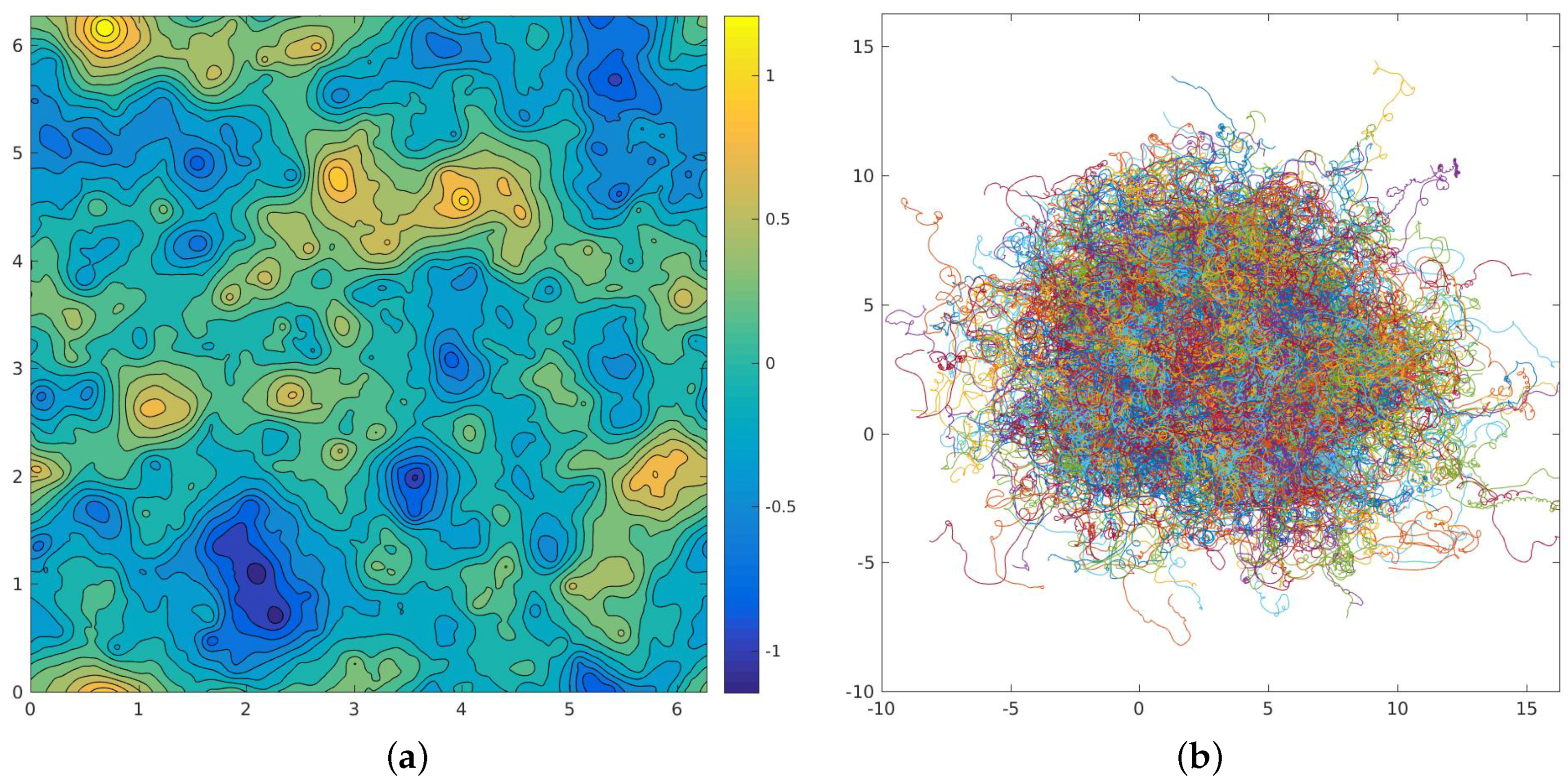
A snapshot of the streamfunction in the equilibrated state from one run is shown in the left panel of Figure 4. The forcing was applied in the wavenumber range $K=[30,35]$ and the Rayleigh coefficient was $R=0.1$. There are numerous large eddies, but smaller scale features are seen as well. The large eddies exceed the forcing scale ($2\pi /30\approx 0.05$), suggesting an inverse energy cascade (e.g., [34]).

When the stationary state was reached, 2000 particles were deployed on a uniform grid and advected with a fourth-order interpolation scheme. The initial particle separation was $r_0=0.01$, comparable to the model grid size. The trajectories are shown in the right panel of Figure 4.

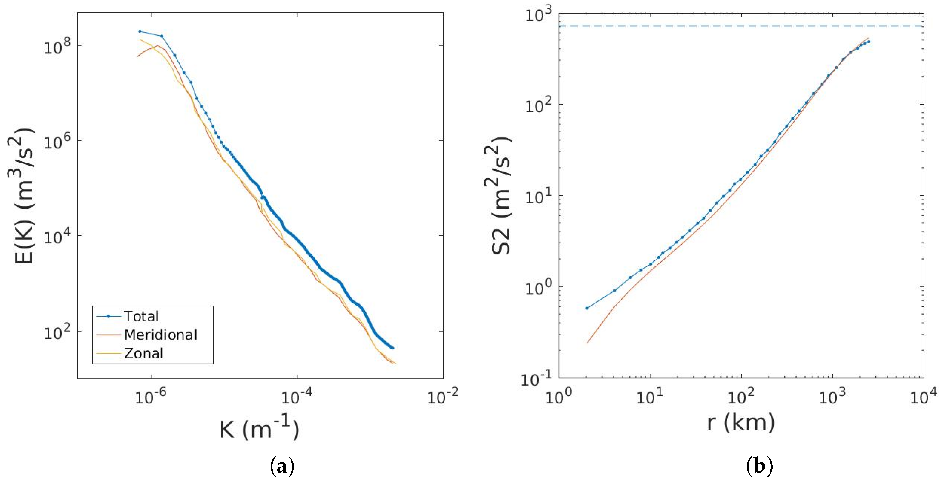
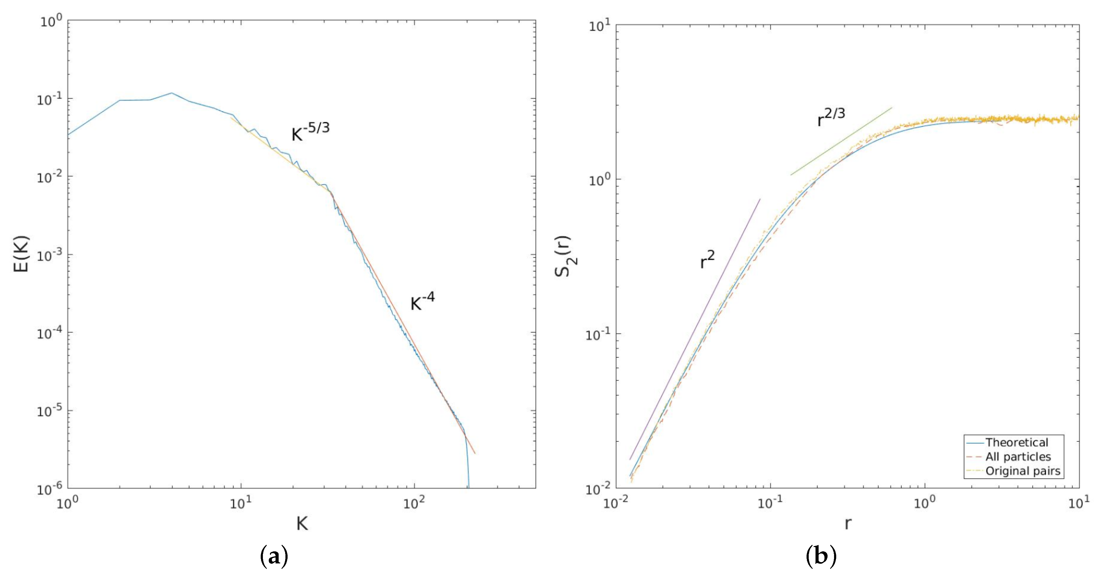
The time-average energy spectrum was shown in Figure 9 of [17] and is reproduced in the panel of Figure 5a. The spectrum is steep from the forcing range ($K=[30,35]$) to roughly $K=200$, where the exponential filter is acting. The slope is nearly $-4$ and is thus greater than the theoretical value ($-3$) for a 2D enstrophy range [35]. This is due to the Rayleigh damping; simulations without this produce a slope closer to $-3$, as seen below. The spectrum is nevertheless non-local above the forcing wavenumber, implying the same impact on pair separations as in an enstrophy range [9]. There is also a short energy range, with a slope of $K^{-5/3}$, from the forcing wavenumbers up to $K=10$. This is in line with an inverse energy cascade, as inferred from Figure 4.

The second-order longitudinal structure functions are shown in the right panel of Figure 5. Three curves are plotted. One (blue solid) is that predicted from the energy spectrum using (14). The second (red dashed) was obtained using velocity differences from all particle pairs in the flow. The third (yellow dash-dot) was calculated using velocities only from pairs deployed together, “original pairs” in the terminology of [13].

The three curves are very similar. All increase nearly as $r^2$ from the grid scale ($r=0.01$) up to the forcing scale ($r=0.1$). The curves flatten out above $r=1.0$. The $r^{2/3}$ dependence expected for an energy range is not seen, due most likely to its limited wavenumber extent. However, all three estimates are very similar. This implies that the choice of original or “chance” pairs does not yield qualitative differences in $S_{2l}$; it merely effects the number of samples (there are many more chance pairs).

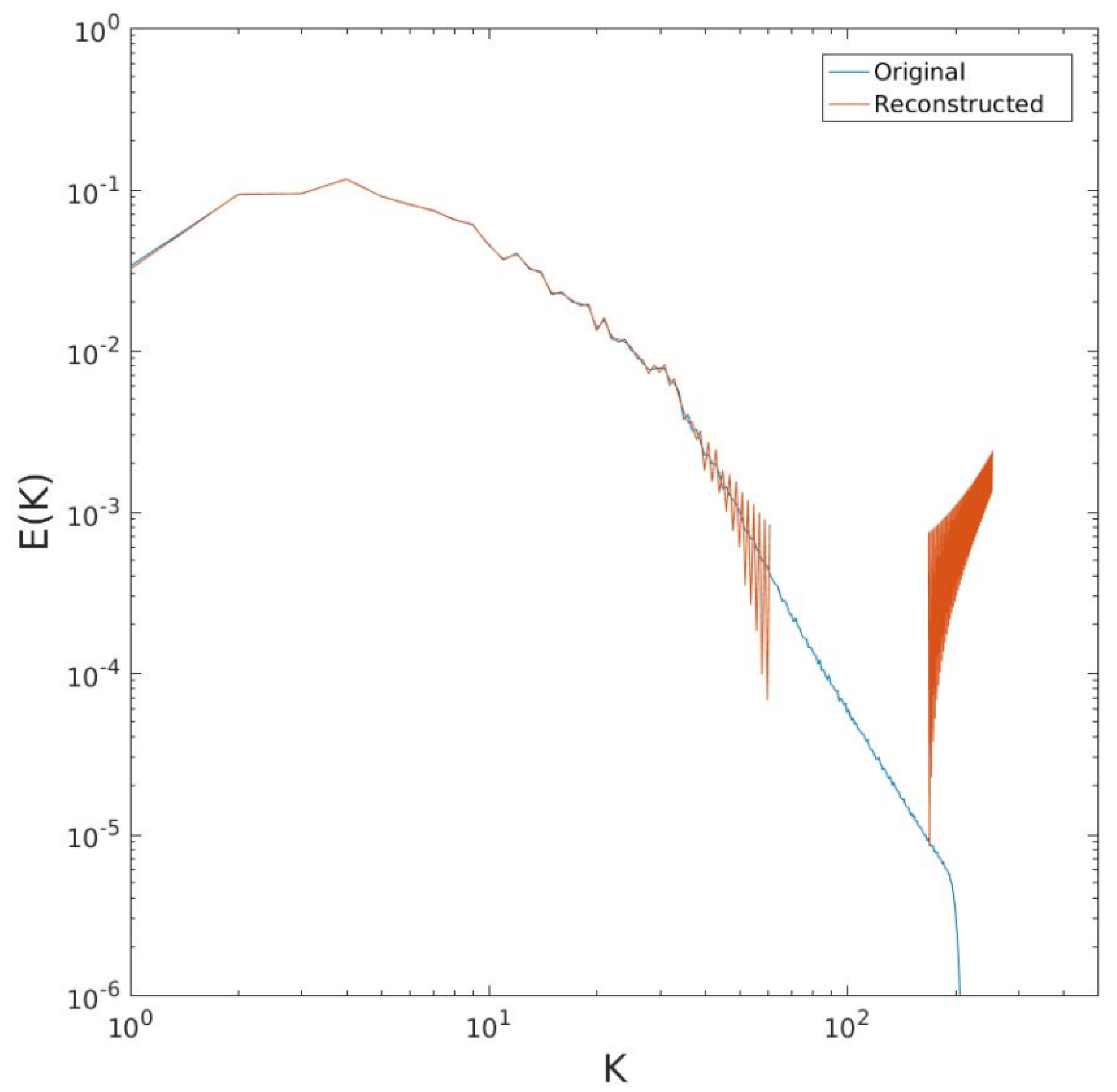
To test the transform (15), we first use the structure function calculated from the energy spectrum. We do this numerically. (Cree and Bones [36] discuss the numerical evaluation of Hankel transforms. In such cases, the transform integral is (necessarily) truncated at a finite upper limit. To accommodate this, the transformed function is assumed to vanish above this scale/wavenumber. Appropriate choices of equally-spaced separations and wavenumbers are also made. We employ Hankel functions which are available in Matlab (www.mathworks.com)). Of course, this is just a test of the invertibility of the Hankel transforms linking the two measures. The result is shown in Figure 6. The reconstruction is good in the wavenumber range below the forcing range, but at higher wavenumbers, the predicted spectrum deviates from the original substantially, even becoming (nonphysically) negative at some wavenumbers.

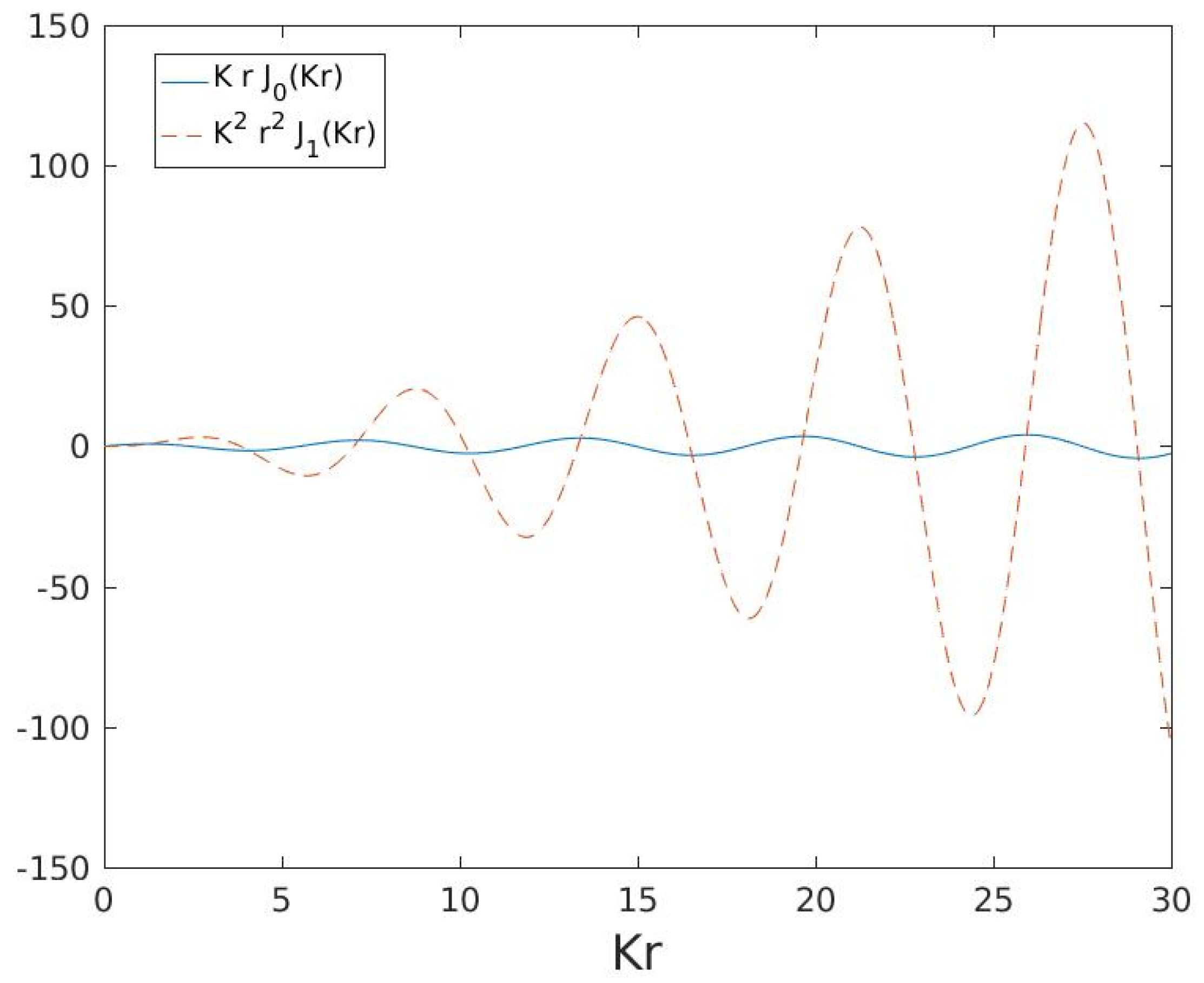
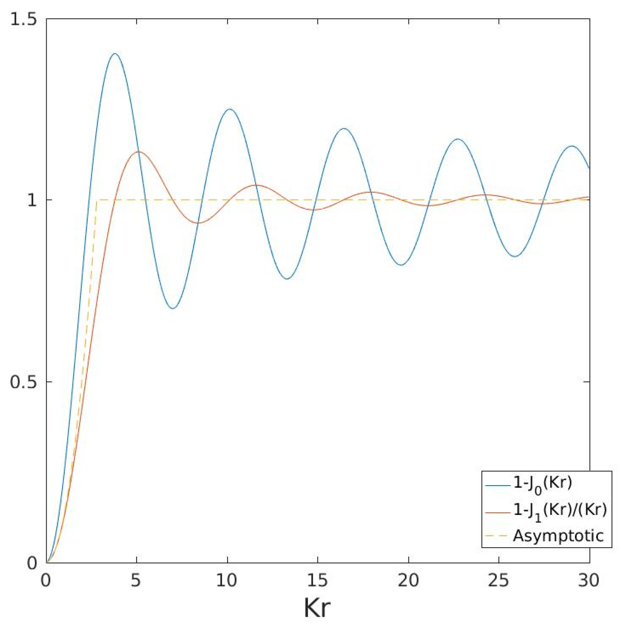
The failure at large wavenumbers is due to the filter function in (15), $K^2{r}^2{J}_1\left(Kr\right)$. As seen in Figure 7, this oscillates and grows with separation, asymptotically as ${\left(Kr\right)}^{3/2}$. Thus, the small wiggles present in the structure function where it levels off (Figure 5) affect the energy spectrum, particularly at large wavenumbers. Note this is not a consequence of integrating the Hankel transform over a finite range of wavenumbers; it is rather due to having a blue filter function, which magnifies noise at large separations.

Thus, we explored an alternate approach. The longitudinal velocity correlation, $f\left(r\right)$, is easily obtained from the second-order structure function from (13). One can then calculate the two-point correlation, $R_{ii}\left(r\right)$, using (8), and the energy spectrum follows from (4). This is preferable to (15) because the filter in (4), $Kr{J}_0\left(Kr\right)$, increases more slowly (Figure 7), asymptotically only as ${\left(Kr\right)}^{1/2}$.

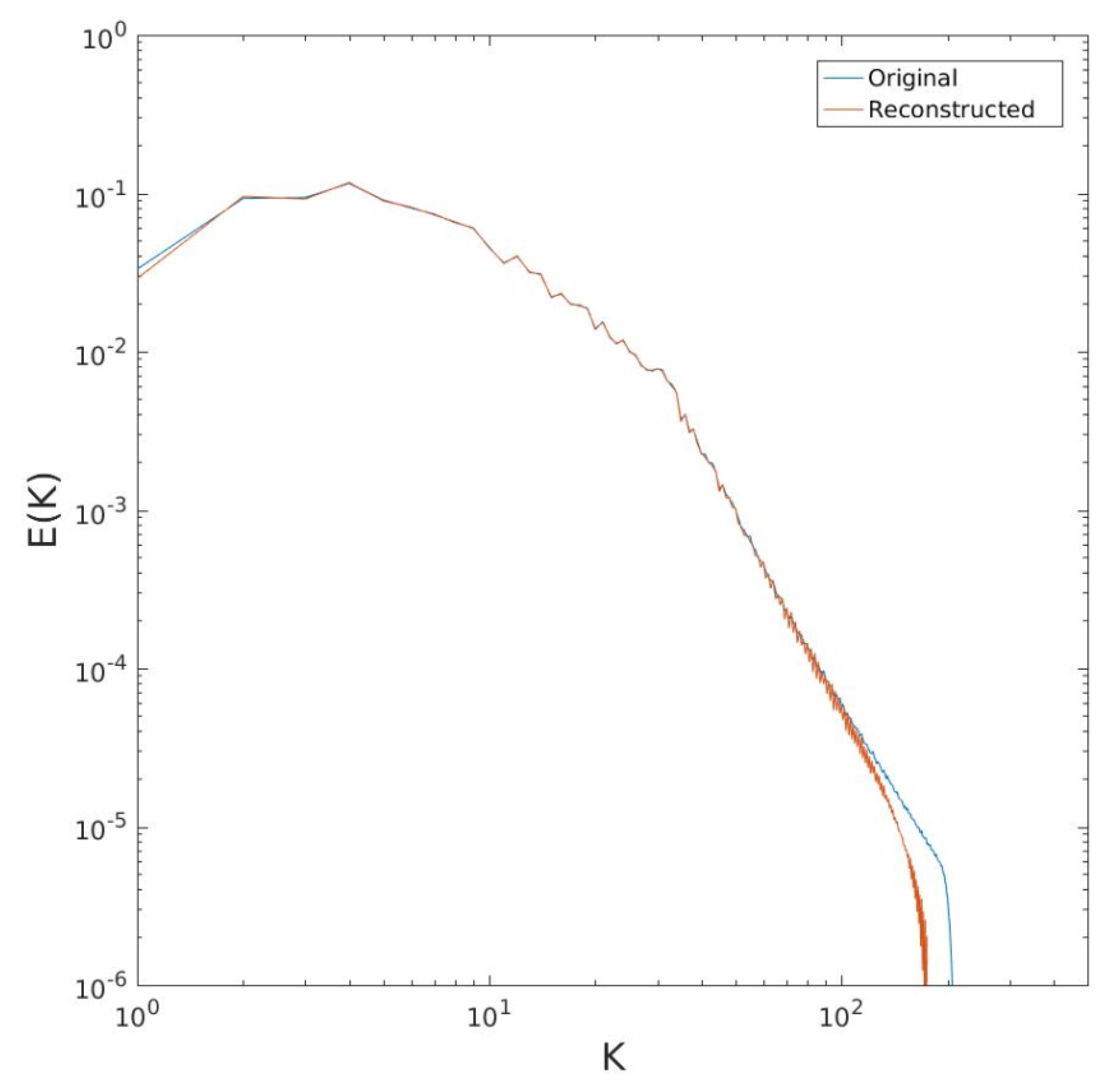
The spectrum obtained using this alternate approach is shown in Figure 8. Now, a greater range of wavenumbers is reproduced, up to roughly $K=100$. Hence, this approach produces a more satisfactory inversion, and we use it hereafter.

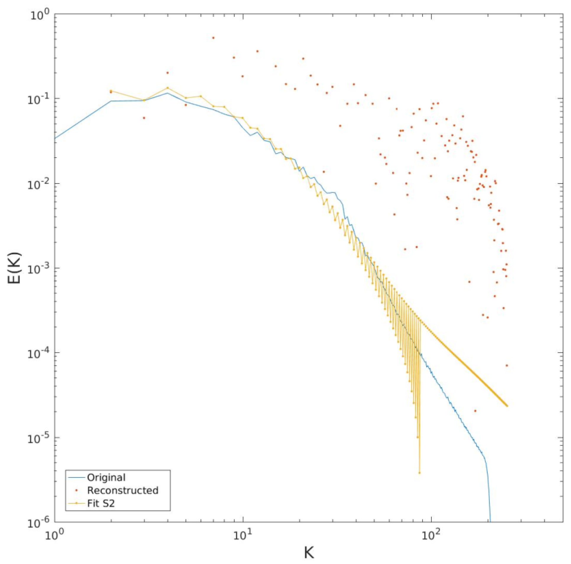
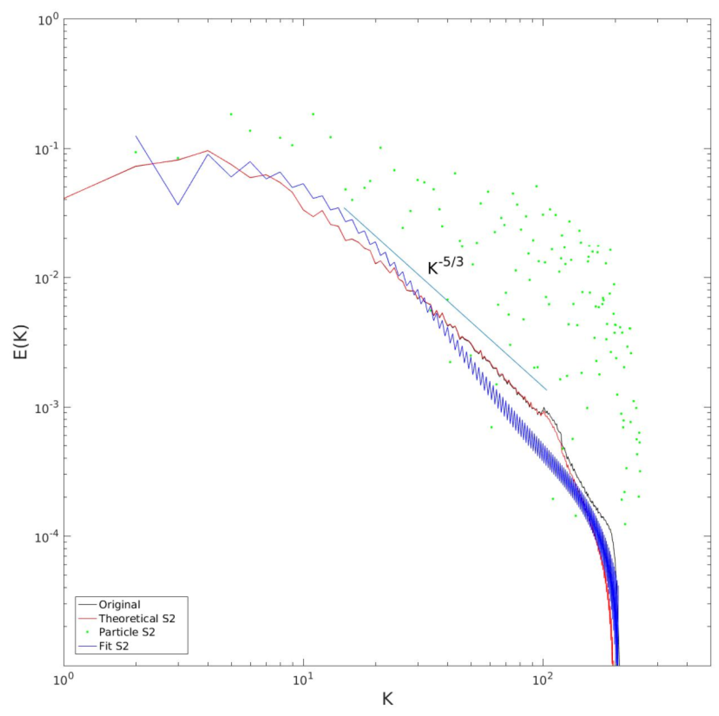
Next, we turn to the particle-derived structure functions. For this, we use the structure function obtained from all particle pairs (the results with the original pairs are similar but noisier). The reconstructed spectrum is very noisy, as indicated by the red dots in Figure 9. The spectrum has energies that are also greatly in excess of the actual values. These contributions are accompanied by negative spectral values, not shown in the figure. This again is due to the inversion (4), amplifying variations in the structure function at large separations. In this case, those variations (which are both positive and negative, as seen below) are large enough to corrupt the spectrum over nearly the entire range of wavenumbers.

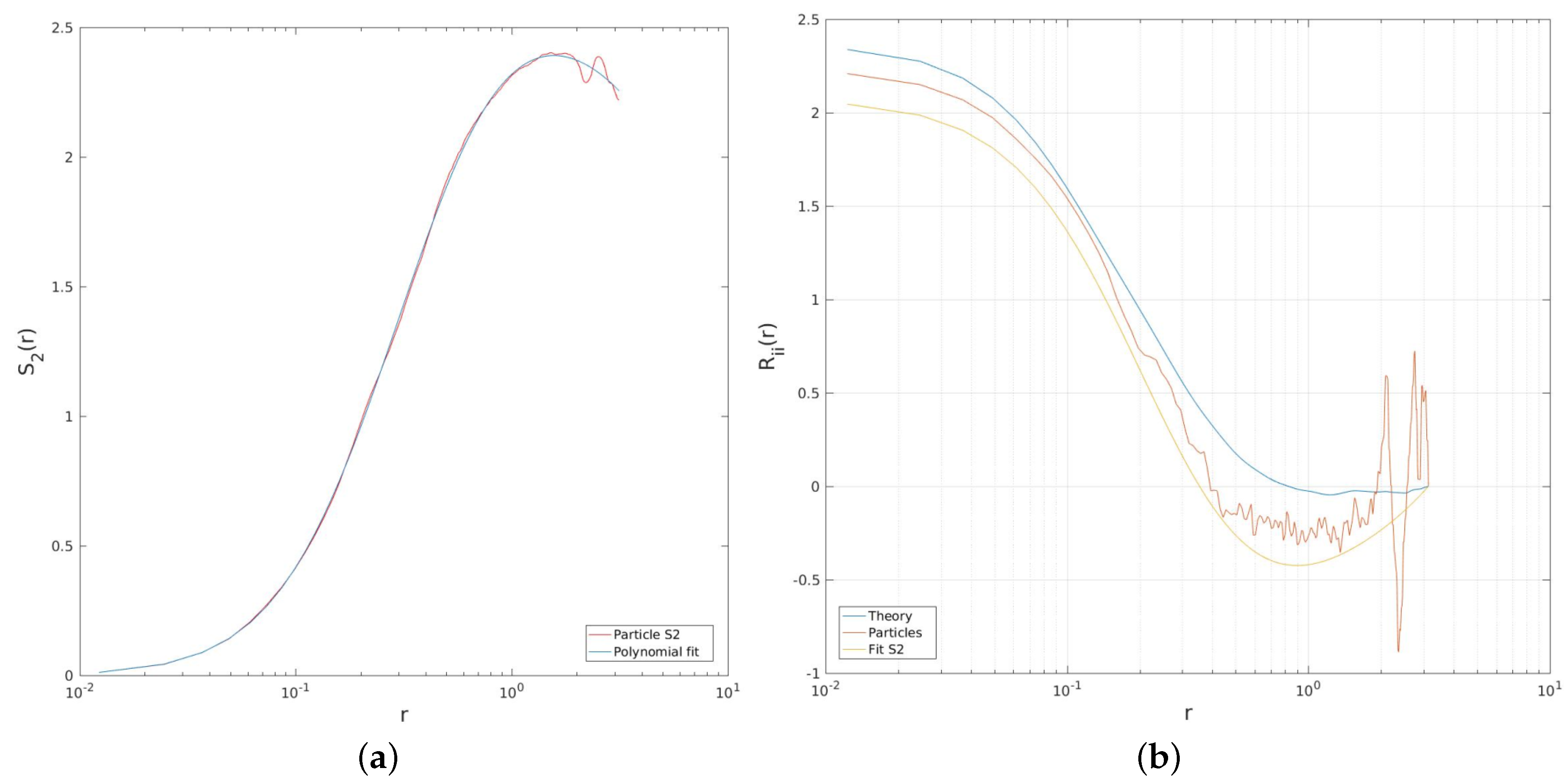
The results are improved if the structure function is fit to a polynomial, to remove oscillations at large separations. We did this by fitting the logarithm of $S_{2l}$ with a sixth-order polynomial, as shown in the panel of Figure 10a. As seen, the behavior at small scales is well captured by the fit while the wiggles at large scales are eliminated.

Shown in the right panel are the two-point correlations, $R_{ii}\left(r\right)$, from the raw particle-derived $S_{2l}$ (in red) and from the polynomial fit (in yellow). Also plotted is the two-point correlation obtained from the transformed $S_{2l}$ (i.e., that obtained from the transform of the spectrum), in blue (all three correlations have been adjusted so that the last value is zero, as expected for the Hankel transform [36]). The particle-derived correlation is similar at small separations but is much noisier at larger separations, oscillating between positive and negative values. These oscillations result in the large positive and negative spectral values in Figure 9. The polynomial fit remedies this somewhat by removing the oscillations. However, the resulting correlation still differs from the curve obtained with the transformed $S_{2l}$.

Using the two-point correlation from the polynomial fit in (4) yields the spectrum plotted in yellow dots in Figure 9. This still exhibits oscillations which grow with wavenumber, but the result is significantly improved over the estimate using the raw structure function. That said, one is not able to detect the two inertial ranges present in the original spectrum (Figure 5).

The results from two other simulations are shown in Figure 11 and Figure 12. The first is for a pure energy cascade, forced in the range $K=[100,120]$, with a Rayleigh coefficient of $R=0.1$. Plotted are the original spectrum (in black), the reconstruction from the transformed $S_{2l}$ (in red), from the raw particle-derived $S_{2l}$ (green dots) and from a sixth-order polynomial fit of the latter (blue). The original spectrum exhibits a well-defined $K^{-5/3}$ inertial range from the forcing range down to $K=10$. The spectrum from the transformed $S_{2l}$ matches the original to roughly $K=100$, as in the previous case. The spectrum from the raw $S_{2l}$ is again noisy, while that from the polynomial fit is closer to the actual spectrum. However, the latter is also steeper than the true spectrum, giving an incorrect estimate of the slope in the inertial range.

The results with a pure enstrophy cascade, forced in the range $K=[1,5]$, are significantly worse (Figure 12). The slope in the inertial range is close to, though slightly steeper than, $K^{-3}$ (there is no Rayleigh damping in this simulation). Significantly, the spectrum from the transformed $S_{2l}$ (red dotted curve) is accurate only at the smallest wavenumbers. It begins to oscillate around $K=10$ and these oscillations increase with wavenumber (the dotted curve indicates the upper branch of the curve, and the lower values are negative). The spectrum derived from the polynomial fit (blue dotted curve) deviates from the original spectrum at even smaller wavenumbers, and exhibits negative values even below $K=10$. The upper branch mirrors that from the transformed $S_{2l}$, but the values are roughly 10 times larger. The spectrum from the raw data (green dots) is again poor.

The results with a non-local spectrum are poorer because the structure function is steeper at the smallest separations, growing nearly as $r^2$ (Figure 2). As such, the larger separations have a proportionally greater impact on the spectral transform than with a local spectrum, degrading the spectrum at smaller wavenumbers.

Averaging the spectral values in logarithmically-spaced bins produced estimates closer to the observed spectrum (not shown), but the results remained fairly poor. Other fits, of both the structure function and the two-point correlation, were also attempted with similar results. Generally, the polynomial fit described above yielded the best results.

Thus, the transform essentially fails for non-local spectra. It may be in the future that more refined methods of filtering the structure functions will be more successful, but the differences between the particle-derived correlation and the theoretical one (Figure 10) suggests this is unlikely.

6. Discussion and Conclusions

Relations between the kinetic energy spectrum and the second-order velocity structure function were derived in two dimensions. These are related to those given by [9] but are specifically applicable to longitudinal structure functions, which are easily measured with pairs of particles. The relations involve Hankel transforms, and can be evaluated with routines found in Matlab.

Structure functions derived from idealized, power-law spectra exhibit power-law dependencies on separation as described previously (e.g., [9,10]). However, the results with inertial ranges of finite extent can differ from those derived assuming infinite ranges. This probably explains why the $r^2$ dependence is rarely observed in situations where the spectra are believed to be non-local (e.g., [37]). We also applied the transform to the kinetic energy spectrum in the upper troposphere of [18]. The resulting second-order structure function closely resembles the longitudinal structure function calculated previously with the same data by [26].

The relations were then applied to data from several 2D turbulence simulations. First, the structure function was calculated from the spectrum using (14), and then the inverse relation (15) was used to recover the energy spectrum. The spectrum was reproduced at small wavenumbers but not at large wavenumbers because the Hankel transform (15) has a filter that magnifies contributions from large separations. However, calculating the two-point velocity correlation first and then using (4) produced a spectrum which matched the original over most of the wavenumber range.

The problems associated with large separations are amplified when using particle-derived structure functions, which are noisy precisely at the largest scales. The spectral estimates are improved if one fits the structure functions with a high-order (6th in this case) polynomial, but they deviate nonetheless from the original spectra. The results also are better when the spectra are local (shallower than $K^{-3}$). The transform functions poorly with non-local spectra because the large separations have a relatively greater contribution to the integrated structure function. It may be that more sophisticated data processing could improve this situation.

Thus, the transform from spectrum to structure function is more robust than the inverse. This follows from the difference in the filtering inherent in the two operations. While the filter asymptotes to one for large separations with the spectral transform (14), it increases with separation for the inverse transform (4). A similar issue pertains in three dimensions, as seen in Equations 3.4.16 of [24]. Thus, it is easier working with the forward transform to assess a given structure function, like that of Lindborg’s, than to do the inverse.

The present results also suggest that it is probably better to examine structure functions with Lagrangian data than to extract energy spectra. As seen here, the structure functions are fairly robust, agreeing well regardless of whether chance or original pairs are used. Nevertheless, structure functions integrate contributions across wavenumber and are certainly not as “clean” as energy spectra.

Several recent studies have examined decomposing energy spectra into rotational and divergent components [29,38,39]. This usefully separates contributions from large-scale balanced motions (e.g., vortices) and small-scale phenomena like waves. A similar decomposition can be applied to structure functions [40,41]. The present relations can be used to test consistency between the two, as shown here in relation to the atmospheric spectra.