Uncertainty Quantification at the Molecular–Continuum Model Interface  ^†

Abstract

Non-equilibrium molecular dynamics simulations are widely employed to study transport fluid properties. Observables measured at the atomistic level can serve as inputs for continuum calculations, allowing for improved analysis of phenomena involving multiple scales. In hybrid modelling, uncertainties present in the information transferred across scales can have a significant impact on the final predictions. This work shows the influence of force-field variability on molecular measurements of the shear viscosity of water. In addition, the uncertainty propagation is demonstrated by quantifying the sensitivity of continuum velocity distribution to the particle-based calculations. The uncertainty is modelled with polynomial chaos expansion using a non-intrusive spectral projection strategy. The analysis confirms that low-order polynomial basis are sufficient to calculate the dispersion of observables.

1. Introduction

Recent years have seen a large number of publications devoted to atomistic–continuum hybrid modelling (for a review, see Teschner et al. [1]). Emerging strategies which combine disparate length and time-scales allow us to tackle numerical limitations and enable better understating of complex physical and biological processes. High-fidelity simulations that aim to accurately describe the fluid flow behaviour are beginning to take advantage of particle-based methods for analysing system properties or detailed physics at interfaces while modelling the bulk of the domain with an efficient Navier–Stokes solver. A major challenge in hybrid modelling is the quality of the information exchanged between domains, as well as the efficiency of the inter-scale communication. Molecular dynamics (MD) is a powerful tool for capturing phenomena at the atomic level [2,3,4,5], but the method relies on the accuracy of the potential (or force-field) with which the inter-atomic forces of a real system can be reproduced [6]. A widely used model of molecular interactions is the Lennard-Jones (LJ) potential, defined for particles located at ${\mathbf{r}}_i$ and ${\mathbf{r}}_j$ as [7]:

$$U\left(r_{ij}\right)=\left\{\begin{array}{cc}4ϵ\left[\begin{array}{c}{\left(\frac{\sigma }{r_{ij}}\right)}^{1}2-{\left(\frac{\sigma }{r_{ij}}\right)}^6\end{array}\right]& r_{ij}<r_c,\\ 0& r_{ij}\ge r_c,\end{array}\right.$$

(1)

where $r_{ij}\equiv \left|{\mathbf{r}}_{ij}\right|$, ${\mathbf{r}}_{ij}={\mathbf{r}}_i-{\mathbf{r}}_j$ and $r_c$ is a cut-off radius beyond which the interactions are neglected. The parameters of the LJ model, the depth of the potential well (ϵ), and the distance of zero inter-potential energy (σ) are estimated through quantum chemistry calculations or fitted to match the experimental data. Large discrepancies in developed force-fields are the main source of uncertainty, resulting in often different predictions; as stated by Ouyang and Bettens [8], the existence of over 40 water MD models indicates the challenge of reproducing the properties of real liquids.

Sullivan [9] describes two common categories of uncertainty in physical and numerical experiments: aleatoric and epistemic. The first type refers to uncertainty due to the physical variability of a system (irreducible), while the latter arises from a lack of knowledge (reducible). The epistemic uncertainty can further be subdivided into model form uncertainty, where the correctness of the strategy is questioned, and parametric uncertainty caused by lack of confidence that the chosen values are the best to represent certain properties. A common objective of uncertainty quantification (UQ) is to analyse a stochastic model’s response to variable inputs (forward propagation) or to determine the value of input parameters which correspond to a given observation (inverse problem). Traditionally, the sensitivity analysis of system parametrisation has been conducted using Monte Carlo sampling. Although very powerful, the convergence rate of the method is slow, $O\left(M^{-1/2}\right)$, where M is a number of realisations/trials, resulting in high computational cost [10]. An alternative approach is based on spectral representations of observables allowing for higher efficiency of the analysis. Parametric uncertainty can be modelled with the polynomial chaos (PC) method [11], which in its generalised form (gPC) [10] describes an expansion of a random variable stochastic process over a probability space $(\mathsf{\Omega },\mathcal{F},\mu )$ with respect to an appropriate orthogonal polynomial basis of $L^2(\mathsf{\Omega },\mu ;\mathbb{R})$. Here Ω defines a sample space which contains all possible outcomes, while $\mathcal{F}$ is a σ-algebra (a set of events), and μ is the probability measure which defines event’s likelihood. Given a functional representation of quantities of interest (QoI), statistical post-processing is then straightforward. In addition, the higher the regularity of the approximated function, the faster the convergence of the truncated expansion.

It is worth noting that there are other surrogate-based methods. The approach used depends not only on computational resources or the problem specifications, but also on particular expertise or background. While polynomial chaos is a popular choice in the applied mathematics and engineering community, different techniques have gained recognition in other fields; for example, Gaussian process emulator [12] or Bayes linear surrogate [13] are principally used in statistics, while a neural network approach [14] is becoming popular among physicists. In our work, we focused on incorporating a polynomial chaos solution in order to validate the results with published studies in the field of fluid mechanics. However, we plan in future to explore different surrogate models for uncertainty quantification analysis. We are particularly interested in a Gaussian process emulator which has recently been reported to outperform the polynomial-based approach [15,16].

Since the work of Xiu and Karniadakis [17], the use of polynomial chaos to represent the uncertainty of the input in Navier–Stokes flow simulations has been growing [18]. However, the application of the probabilistic methodology to particle-based simulations—or atomistic–continuum modelling—is still recent [6]. Rizzi et al. [19] exploited the polynomial chaos expansions and Bayesian inference [20] to develop a framework for sensitivity analysis of MD measures of diffusivity, density, and enthalpy to parameters of the TIP4P water model [21]. Further research on the reliability of MD predictions involved the analysis of parametric uncertainty on the flux of ions through silica nanopores [22,23]. Jacobson et al. [24] applied generalised polynomial chaos to assess the accuracy of a family of coarse-grained water models. A recent study by Salloum et al. [25] focused on a two-way coupling of uncertainty across scales with the use of surrogate models for computational efficiency. The studies showed the benefit of using a polynomial chaos expansion to validate the results and explore the parametric dependence of final predictions, enabling the development of improved fluid modelling. Mentioned works stressed that the main source of uncertainty in molecular dynamics was due to the atomistic force fields, with the intrinsic noise making only a minor contribution. However, filtering particle-based data can lead to more efficient information extraction and intra-scale communication; a review of various signal processing methods for molecular simulations can be found in Zimoń et al. [26,27].

In this work, a non-intrusive strategy of polynomial chaos is used to determine the influence of uncertainty in Lennard-Jones potential on non-equilibrium MD-based viscosity calculation of water (TIP4P/2005 model [28]). Although the UQ analysis of this kinetic property is important for parametrising the forcefield, it has not yet been considered in the literature. In addition, the probability distribution of the viscosity is propagated through the simulation of classical Stokes flow in order to analyse the sensitivity of final velocity prediction. The overall study enables us to verify the previously reported results on polynomial chaos expansion for fluid simulations and contribute to the development of high-fidelity multi-scale modelling. This article is organised as follows. In Section 2, the theory of polynomial chaos is briefly outlined. In Section 3, the simulation set-up and the uncertainty quantification propagation in modelling components are described, followed by results and discussion. Concluding remarks are provided at the end.

2. Mathematical Background

Given the uncertain input—in this study the LJ parameter $ϵ\left(\xi \right)$, where ξ has a certain probability measure μ on $\mathsf{\Omega }\subseteq \mathbb{R}$, a real-valued random variable Y—the MD prediction of QoI can be represented as a PC expansion as follows:

$$Y\left(\xi \right)=\sum _{k=0}^{\infty }{y}_k{\psi }_k\left(\xi \right),$$

(2)

where the basis functions ${\psi }_k$ are orthogonal with respect to measure μ and ${\left\{y_k\right\}}_{k=0}^{\infty }$ is a set of PC coefficients. The study can be extended to the ${\mathbb{R}}^n$-valued random variable, $\mathbf{Y}=\{Y_1,\cdots ,Y_n\}$, where

$$\mathbf{Y}\left(\xi \right)=\sum _{k=0}^{\infty }{\mathbf{y}}_k{\psi }_k\left(\xi \right),$$

(3)

with ${\mathbf{y}}_k=\{y_{1,k},\cdots ,y_{n,k}\}\in {\mathbb{R}}^n$ for each $k\in {\mathbb{N}}_0$; dependence of QoI on multiple sources of uncertainty $\mathit{\xi }=\{{\xi }_1,\cdots ,{\xi }_{\alpha }\}$, can also be considered. In practice, the series expansion is truncated after $P+1=(\alpha +p)!/\alpha !/p!$ terms, where α defines the stochastic dimensionality and p is the order of the corresponding multivariate polynomials, ${\mathsf{\Psi }}_k\left(\mathit{\xi }\right)$. Such representation (including the truncated series) allows for straightforward stochastic post-processing; the measurement of the expected value of Y is simply its zeroth PC coefficient, $\mathbb{E}\left[Y\right]〈{\mathsf{\Psi }}_{0}Y〉={\sum }_{k=0}^P{y}_k〈{\mathsf{\Psi }}_0{\mathsf{\Psi }}_k〉=y_0$, while the variance is defined as

$$\mathbb{V}\left[Y\right]=\mathbb{E}\left[|Y-\mathbb{E}\left[Y\right]{|}^2\right]=\sum _{k=0}^P{y}_k^2〈{\mathsf{\Psi }}_k^2〉.$$

(4)

Wiener [11] introduced PC expansions, where Hermite polynomials were used to model stochastic processes with Gaussian random variables. The extension to generalised PC developed by Xiu and Karniadakis [29] allows for non-Gaussian random processes. In the gPC approach, different orthogonal polynomials in the Askey scheme are incorporated for different distribution types. In this work, the abbreviation PC refers to a generalised formalism of Wiener’s approach.

Considering its practical implementation, there are two main strategies for determining the expansion coefficients, $y_k$, in Equation (2). The PC expression of random variables can be directly introduced to the model equations, and a Galerkin projection is then applied to obtain a stochastic solver [9,10]; hence, the approach is referred to as the intrusive spectral projection (ISP). Xiu [10] explains that although the Galerkin formalism offers the most accurate solutions, it is not suitable for highly complex models. It is also not recommended when the UQ analysis is performed on legacy codes, which are often not amenable to changes. The opposite situation is for non-intrusive methods which rely on individual realisations of Y to determine the response of the system to random inputs. In this approach, the deterministic solution does not need to be modified and can be evaluated at any desired point of the probability space $(\mathsf{\Omega },\mathcal{F},\mu )$. If the normalisation constant, ${\gamma }_k=\langle {\mathsf{\Psi }}_k^2\rangle$, is known, in non-intrusive spectral projection (NISP), the PC coefficients

$$y_k=\frac{〈Y{\mathsf{\Psi }}_k〉}{〈{\mathsf{\Psi }}_k^2〉}=\frac{1}{{\gamma }_k}\int Y\left(\xi \right){\mathsf{\Psi }}_k\left(\xi \right)d\mu \left(\xi \right),k=0,\dots ,P$$

(5)

can be obtained by approximating the integral with quadrature rules. The realisations of Y are used to determine a surrogate model $\tilde{Y}$ for which

$$\tilde{Y}=\sum _{k=0}^P{\tilde{y}}_k{\mathsf{\Psi }}_k\approx Y,$$

(6)

where ${\tilde{y}}_k=\frac{1}{{\gamma }_k}{\sum }_{j=1}^{Q}y\left({\xi }^{\left(j\right)}\right){\mathsf{\Psi }}_k\left({\xi }^{\left(j\right)}\right)w^{\left(j\right)}$, while $\left({\xi }^{\left(j\right)},w^{\left(j\right)}\right)$ are the prescribed nodes and their corresponding weights. If the normalisation constant, ${\gamma }_k$, can be described by polynomials of degree less than or equal to $(2Q-1)/2$, where Q is the number of quadrature nodes, then the PC coefficients can be exactly determined. Sullivan [9] states that if the dimensionality of vector ξ is small and $Y\left(\xi \right)$ is relatively smooth, the Gaussian quadrature approximation (nodes at the roots of μ-orthogonal polynomials) is an optimal choice. In this work, the NISP is performed with the open-source tool Chaospy [30].

3. Problem Description

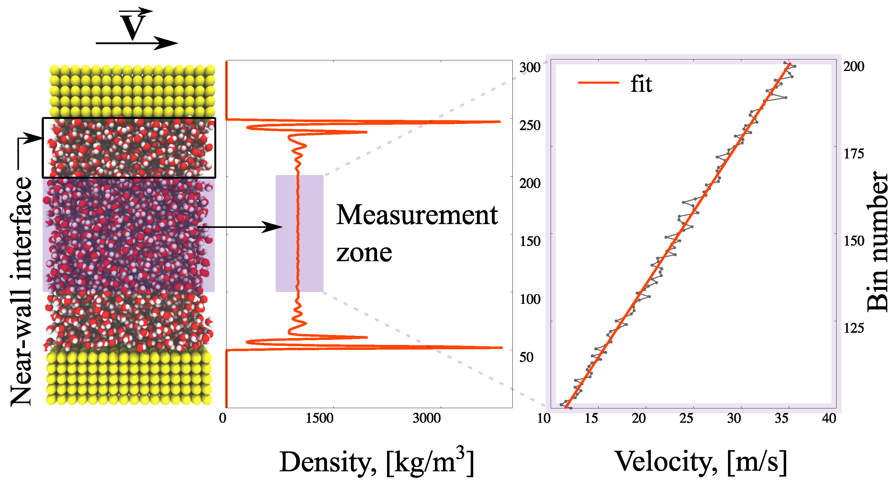
3.1. Viscosity Calculation with Non-Equilibrium Molecular Dynamics (NEMD)

Computational simulations play an important role in the interpretation of experimental results. In many studies, the transport coefficients are assumed to be constant, depending only on the temperature and density of the fluid, without considering local behaviour such as the dependence of shear viscosity on the velocity gradient [7]. Achieving high accuracy and precision measurements of such properties is not a simple task. However, valuable knowledge of a material’s rheological characteristics can be obtained with molecular dynamics. Particle-based modelling offers an ideal environment to analyse the viscous nature of a fluid without some of the constraints of experimental studies [31,32,33].

There are two main strategies for calculating transport coefficients: by performing non-equilibrium molecular dynamics or using the equilibrium Green–Kubo (GK) formalism [34]. The main benefit of the first approach is its fast convergence, making it a popular choice for estimating the shear viscosity. In this work, a sensitivity analysis to the LJ potentials of NEMD calculations is undertaken. The results are obtained by simulating a Couette flow where a constant shear stress is induced in water confined between two parallel silicon walls by the constant motion of the upper boundary. All molecular simulations are performed using the mdFoam solver [35,36] developed in OpenFOAM [37]. A popular TIP4P/2005 water model was chosen for the analysis, as it gives the best prediction of the viscosity for the complete range of temperatures. As previously mentioned, the value of the potential well is assumed to be uncertain, $ϵ\left(\xi \right)$, where $\xi \sim \mathcal{U}({ϵ}_{\min },{ϵ}_{\max })$; the support of the distribution is based on the force-fields of other water models from the TIP4P family, ${ϵ}_{\min }\approx 0.84\times {ϵ}_{OO}$ from TIP4P [38] and ${ϵ}_{\max }\approx 1.14\times {ϵ}_{OO}$ from TIP4P/Ice [39], where ${ϵ}_{OO}=1.287\times {10}^{-21}$ J and ${\sigma }_{OO}=3.1589$ Å are the values of the TIP4P/2005 model introduced by Abascal and Vega [28]. The solid–liquid interaction is modelled following the common Lorentz–Berthelot mixing rule [40], based on the LJ potential of silicon from Ritos et al. [41].

The simulation details are described in Figure 1. The computational domain is divided into a measurement (bulk) zone where the continuum behaviour of the fluid is observed, and interfaces with non-homogeneities caused by the wall presence (note the water layering in Figure 1). The system is modelled as periodic in the x- and z-directions for efficiency. A linear velocity response to the movement of the upper boundary develops in the measurement zone; the calculated shear stress, τ, and velocity gradient, $\delta v/\delta y$, are used to obtain the viscosity coefficient, η

$$\tau =\eta \frac{\delta v}{\delta y}.$$

(7)

Averaged values of observables are measured in 300 horizontal bins of thickness 0.32 nm every $4000\mathrm{\Delta }t$ to avoid redundancy, where the time-step is set to $\mathrm{\Delta }t=2$ fs. The simulations are performed in a (canonical) NVT ensemble (a statistical mechanical ensemble with a fixed number of particles (N), volume (V), and system’s temperature (T)); the temperature of the system is maintained at T = 298 K via the Berendsen thermostat [42]. In order to avoid affecting the velocity calculations, the thermostat is applied only in the z-direction of the flow; the equipartition theorem ensures that each degree of freedom is close to the target temperature. In the equilibration stage, water density is obtained with a FADE controller [43]. After the desired system has developed, the density controller is switched off and the top wall is set to move at $v=47.5$ m/s until a steady-state is reached (high velocities reduce thermal fluctuations); the calculation of velocity takes place in the measurement-zone consisting of 100 bins. The applied shear stress is measured using the Irving–Kirkwood equation [44].

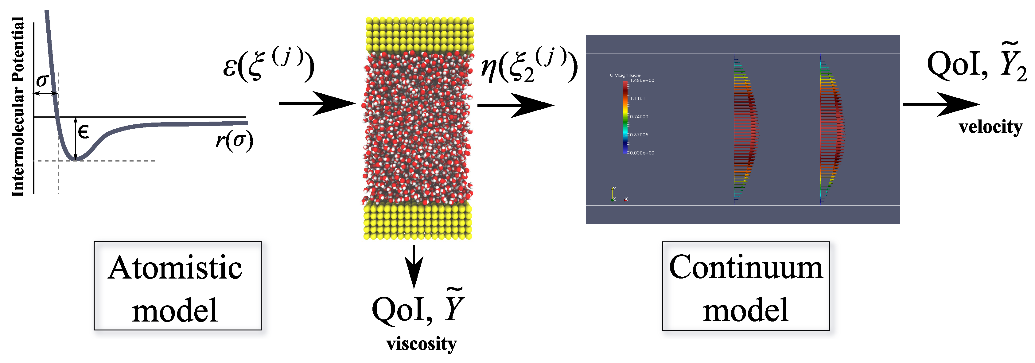
3.2. Non-Intrusive Uncertainty Quantification in Multi-Scale Modelling

As mentioned previously, the potential well parameter has been assigned a uniform probability distribution, $ϵ\left(\xi \right)\sim \mathcal{U}({ϵ}_{\min },{ϵ}_{\max })$. The sample points in probability space for which our MD model is evaluated are specified through $p+1$-order Gaussian quadrature selected for given distribution. Having determined nodes, ${ϵ}_1,\cdots ,{ϵ}_{p+1}$, and corresponding weights, we perform the MD simulations and use viscosity results to describe the stochastic response to the uncertain parameter. Polynomials of order p are computed using a three-term recurrence relation [30]. We then use the basis, quadrature nodes, weights, and model samples to create the surrogate model, ${\tilde{Y}}_{\eta }$.

The surrogate model, ${\tilde{Y}}_{\eta }$, is used to construct a response probability density function (PDF). The cost of the procedure is very low in comparison with evaluating the PDF with the original model, $Y_{\eta }$, which requires a full MD simulation. Ten thousand realisations are selected from the ϵ distributions and plugged into the surrogate model. An empirical histogram—or alternatively a kernel density estimate—can then be used to fit one of the standard distributions, which are subsequently applied in the macroscopic simulations.

Two alternatives could be pursued at this stage. Firstly, the kernel density estimate can be directly used in constructing an orthogonal family for the spectral approximation at the macroscopic level. This approach removes the necessity of a fitting procedure. Another alternative is to use evaluated viscosities as nodes for the macroscopic response quadratures, but this procedure hides the multi-scale interface. Step-by-step analysis gives more insight into the response propagation.

An estimated viscosity PDF is then passed onto the continuum calculation as a random input for NISP, $\eta ({\xi }_2^{\left(j\right)})$. In the continuum model, we use a Navier–Stokes solver (OpenFOAM) to obtain the steady-state laminar solution for a 2D-channel with fixed dimensions and flow rate. For the sake of demonstration, we focus on the spatial development of the center-line velocity profile. Uniform fixed-velocity inlet and no-slip on walls are given as boundary conditions. The center-line velocity profile will reach the fully-developed value more quickly for higher viscosities. For each streamwise point, x, a surrogate model, ${\tilde{Y}}_u\left(x\right)$, is obtained.

The procedure for propagating the uncertainty in this multi-scale framework is summarised in Figure 2.

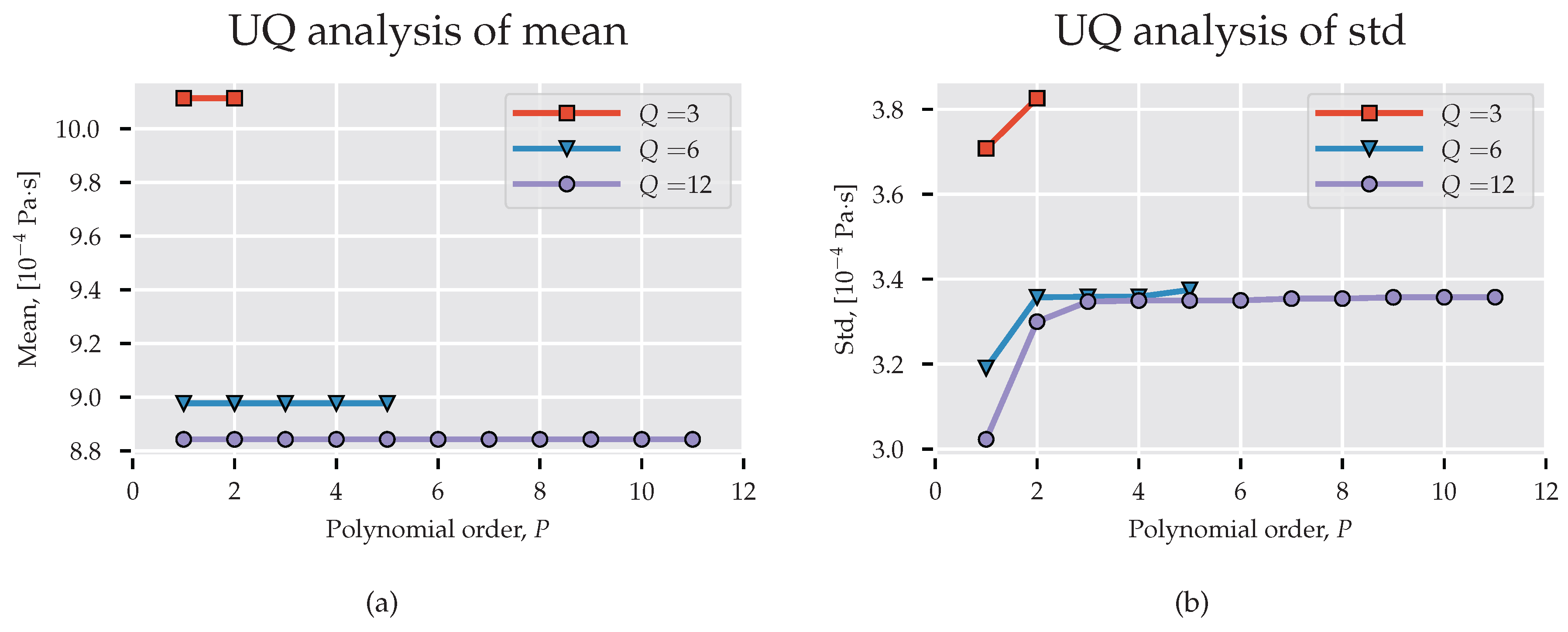
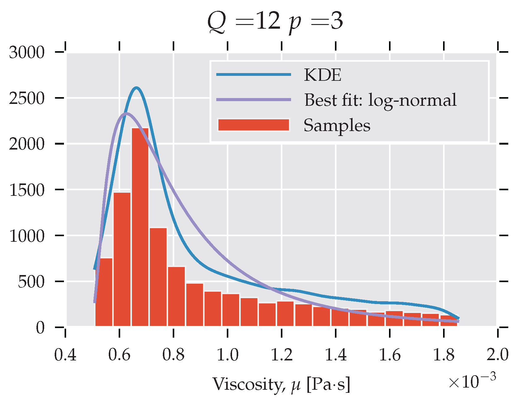
4. Results and Discussion

In the previously mentioned work on UQ in molecular dynamics and multi-scale simulation, it was claimed that low-order polynomials are sufficient to model parametric uncertainty. Rizzi et al. [19] used $Q=7$ quadrature nodes to compute the PC coefficients for density, enthalpy, and self-diffusivity of water with polynomials up to $p=6$. Salloum et al. [25] showed that an expansion order $p=3$ accurately quantifies the uncertainty in molecular dynamics calculation of water velocity. In our study, we consider three PC models of order $p=\{2,3,\dots ,11\}$ with $Q=\{3,6,12\}$ nodes, correspondingly. In Figure 3a,b we present, respectively, mean and standard deviation for spectral projections of increasing order. These pictures verify that a low-order basis is sufficient for determining the stochastic response of the system. Clearly, the first- and second-order statistics measured with $Q=6$ and $Q=12$ are comparable and do not vary significantly for $p\le Q-1$. However, polynomials of order $p=2$ do not provide mean value close to the expected $\eta =8.525\times {10}^{-4}$ Pa·s (the value differs by approximately $4\%$ from the experimental result provided by Harris and Woolf [45] and is within the error bounds of the TIP4P/2005 water model, $8\%$ [46]) obtained with the TIP4P/2005 water model and the standard deviation differs largely from the other estimations.

Subsequently, a third-order polynomial is used to obtain the histogram and kernel density estimates (KDE) describing the viscosity, η. Figure 4 presents the PDF that was obtained for $Q=12$ and $p=3$ with a log-normal fit. Qualitatively similar histograms were obtained for other settings. The histogram exhibits high skewness: the bulk of the mass is situated just below the mean, and large values are vanishing relatively slowly (long tail). This shows that the viscosity estimate is sensitive to the LJ potential parameters. More specifically, a majority of the ϵ from the selected interval underestimates the viscosity, and a large fraction leads to a significant overestimate.

The observation in Figure 4 shows the misrepresentation of the system response in finite order statistics. Even though the mean agrees well with the established value (see Figure 3), the detailed picture provided by the PDF gives a less positive message. The values around the mean are rarely realised if the ϵ parameters are taken from the uniform distribution on the selected interval.

Finally, the identified log-normal distribution is used as an input to a computational fluid dynamics (CFD) analysis. Due to the relatively high skewness of the distribution, the right-most points were only weakly influencing the obtained results. As a result, a quadrature accuracy study was not pursued here, as the fifth order was already reaching machine precision for weights corresponding to larger nodes.

The width of the channel and the velocity at the inlet are fixed to unity, and therefore the center-line velocity varies between 1 and 1.5, with the latter being the fully-developed value. Viscosity affects the distance at which a fully developed value is reached: for high viscosity, the value is reached faster and vice versa. For the lowest viscosity, the channel length of 200 height units was not sufficient to obtain a fully developed velocity profile.

In Figure 5a,b, PDFs for center-line velocity are shown at different spatial positions. The construction follows the same procedure as the PDF for the viscosity, but this time one million samples are used in order to create a smooth transition region. In Figure 5a, each spatial position is normalised with respect to its maximum value to illustrate where the bulk of the mass is situated.

The PDFs derived from PC representations can be used to construct meaningful prediction intervals. As we have seen with the viscosity example, plotting mean and standard deviation as a measure of dispersion could be misleading if the distributions are asymmetrical or multi-modal. Having a PDF allows us to evaluate the relative likelihood of different values in the measured output.

5. Conclusions

In this study, we investigated uncertainty propagation at the interface between molecular and continuum fluid models. Following previous studies, we assume that the potential well coefficient of Lennard-Jones interaction is characterised by a random variable with a uniform distribution. We then characterise the output of the molecular dynamics in terms of standard probability distributions for viscosity and feed that as input to a standard Navier–Stokes solver.

Investigation of increasing quadrature nodes and polynomial order shows that sufficient resolution is reached with low-order bases. The considered polynomial chaos models with $p\ge 3$ result in converged first and second order statistics. With the assumed distribution bounds, standard deviation of molecular observable is approximately $40\%$ of the mean value. These results show how sensitive molecular calculations are to the force field coefficients. Moreover, the PDF of viscosity is asymmetric and highly skewed, suggesting that analysis based solely on an expected value and variance is inadequate.

The study emphasizes the benefits of constructing a surrogate model with an associated stochastic response. It allows an analytical approach to establish confidence in our numerical predictions. A non-intrusive spectral strategy enables this without high computational cost and the need to modify the simulation process. Its significance is particularly visible in hybrid modelling, where additional insight into parametric sensitivity may improve the understanding of multi-scale phenomena.

References

1. Teschner, T.R.; Könözsy, L.; Jenkins, K.W. Progress in particle-based multiscale and hybrid methods for flow applications. Microfluid. Nanofluid. 2016, 20, 1–38. [Google Scholar] [CrossRef]
2. Priezjev, N.V. Effect of surface roughness on rate-dependent slip in simple fluids. J. Chem. Phys. 2007, 127, 144708. [Google Scholar] [CrossRef] [PubMed]
3. Thomas, J.A.; McGaughey, A.J.; Kuter-Arnebeck, O. Pressure-driven water flow through carbon nanotubes: Insights from molecular dynamics simulation. Int. J. Therm. Sci. 2010, 49, 281–289. [Google Scholar] [CrossRef]
4. Piana, S.; Klepeis, J.L.; Shaw, D.E. Assessing the accuracy of physical models used in protein-folding simulations: Quantitative evidence from long molecular dynamics simulations. Curr. Opin. Struct. Biol. 2014, 24, 98–105. [Google Scholar] [CrossRef] [PubMed]
5. Ritos, K.; Borg, M.K.; Mottram, N.J.; Reese, J.M. Electric fields can control the transport of water in carbon nanotubes. Philos. Trans. R. Soc. A 2016, 374, 20150025. [Google Scholar] [CrossRef] [PubMed] [Green Version]
6. Drikakis, D.; Asproulis, N. Quantification of computational uncertainty for molecular and continuum methods in thermo-fluid sciences. Appl. Mech. Rev. 2011, 64, 040801. [Google Scholar] [CrossRef]
7. Rapaport, D.C. The Art of Molecular Dynamics Simulation; Cambridge University Press: Cambridge, UK, 2004. [Google Scholar]
8. Ouyang, J.F.; Bettens, R. Modelling Water: A Lifetime Enigma. CHIMIA Int. J. Chem. 2015, 69, 104–111. [Google Scholar] [CrossRef] [PubMed]
9. Sullivan, T.J. Introduction to Uncertainty Quantification; Springer: Cham, Switzerland, 2015; Volume 63. [Google Scholar]
10. Xiu, D. Numerical Methods for Stochastic Computations: A Apectral Method Approach; Princeton University Press: Princeton, NJ, USA, 2010. [Google Scholar]
11. Wiener, N. The homogeneous chaos. Am. J. Math. 1938, 60, 897–936. [Google Scholar] [CrossRef]
12. Oakley, J.; O’Hagan, A. Bayesian inference for the uncertainty distribution of computer model outputs. Biometrika 2002, 89, 769–784. [Google Scholar] [CrossRef]
13. Goldstein, M. Bayes linear analysis. In Wiley StatsRef: Statistics Reference Online; John Wiley & Sons: Hoboken, NJ, USA, 1999. [Google Scholar]
14. Rojas, R. Neural Networks: A Systematic Introduction; Springer Science & Business Media: Berlin, Germany, 2013. [Google Scholar]
15. Kim, Y.J. Comparative study of surrogate models for uncertainty quantification of building energy model: Gaussian Process Emulator vs. Polynomial Chaos Expansion. Energy Build. 2016, 133, 46–58. [Google Scholar] [CrossRef]
16. Zhou, K.; Hegde, A.; Cao, P.; Tang, J. Design Optimization Toward Alleviating Forced Response Variation in Cyclically Periodic Structure Using Gaussian Process. J. Vib. Acoust. 2017, 139, 011017. [Google Scholar] [CrossRef]
17. Xiu, D.; Karniadakis, G.E. Modeling uncertainty in flow simulations via generalized polynomial chaos. J. Comput. Phys. 2003, 187, 137–167. [Google Scholar] [CrossRef]
18. Montomoli, F.; Carnevale, M.; D’Ammaro, A.; Massini, M.; Salvadori, S. Uncertainty Quantification in Computational Fluid Dynamics and Aircraft Engines; Springer: Cham, Switzerland, 2015. [Google Scholar]
19. Rizzi, F.; Najm, H.N.; Debusschere, B.J.; Sargsyan, K.; Salloum, M.; Adalsteinsson, H.; Knio, O.M. Uncertainty quantification in MD simulations. Part I: Forward propagation. Multiscale Model. Simul. 2012, 10, 1428–1459. [Google Scholar] [CrossRef]
20. Ghanem, R.G.; Doostan, A. On the construction and analysis of stochastic models: Characterization and propagation of the errors associated with limited data. J. Comput. Phys. 2006, 217, 63–81. [Google Scholar] [CrossRef]
21. Jorgensen, W.L.; Chandrasekhar, J.; Madura, J.D.; Impey, R.W.; Klein, M.L. Comparison of simple potential functions for simulating liquid water. J. Chem. Phys. 1983, 79, 926–935. [Google Scholar] [CrossRef]
22. Rizzi, F.; Jones, R.; Debusschere, B.; Knio, O. Uncertainty quantification in MD simulations of concentration driven ionic flow through a silica nanopore. I. Sensitivity to physical parameters of the pore. J. Chem. Phys. 2013, 138, 194104. [Google Scholar] [CrossRef] [PubMed]
23. Rizzi, F.; Jones, R.; Debusschere, B.; Knio, O. Uncertainty quantification in MD simulations of concentration driven ionic flow through a silica nanopore. II. Uncertain potential parameters. J. Chem. Phys. 2013, 138, 194105. [Google Scholar] [CrossRef] [PubMed]
24. Jacobson, L.C.; Kirby, R.M.; Molinero, V. How short is too short for the interactions of a water potential? Exploring the parameter space of a coarse-grained water model using uncertainty quantification. J. Phys. Chem. B 2014, 118, 8190–8202. [Google Scholar] [CrossRef] [PubMed]
25. Salloum, M.; Sargsyan, K.; Jones, R.; Najm, H.N.; Debusschere, B. Quantifying sampling noise and parametric uncertainty in atomistic-to-continuum simulations using surrogate models. Multiscale Model. Simul. 2015, 13, 953–976. [Google Scholar] [CrossRef]
26. Zimoń, M.; Reese, J.; Emerson, D. A novel coupling of noise reduction algorithms for particle flow simulations. J. Comput. Phys. 2016, 321, 169–190. [Google Scholar] [CrossRef]
27. Zimoń, M.; Prosser, R.; Emerson, D.; Borg, M.; Bray, D.; Grinberg, L.; Reese, J. An evaluation of noise reduction algorithms for particle-based fluid simulations in multi-scale applications. J. Comput. Phys. 2016, 325, 380–394. [Google Scholar] [CrossRef]
28. Abascal, J.L.F.; Vega, C. A general purpose model for the condensed phases of water: TIP4P/2005. J. Chem. Phys. 2005, 123, 234505. [Google Scholar] [CrossRef] [PubMed]
29. Xiu, D.; Karniadakis, G.E. The Wiener—Askey polynomial chaos for stochastic differential equations. J. Sci. Comput. 2002, 24, 619–644. [Google Scholar] [CrossRef]
30. Feinberg, J.; Langtangen, H.P. Chaospy: An open source tool for designing methods of uncertainty quantification. J. Comput. Sci. 2015, 11, 46–57. [Google Scholar] [CrossRef]
31. Hess, B. Determining the shear viscosity of model liquids from molecular dynamics simulations. J. Chem. Phys. 2002, 116, 209–217. [Google Scholar] [CrossRef]
32. Sofos, F.; Karakasidis, T.; Liakopoulos, A. Transport properties of liquid argon in krypton nanochannels: Anisotropy and non-homogeneity introduced by the solid walls. Int. J. Heat Mass Transf. 2009, 52, 735–743. [Google Scholar] [CrossRef]
33. Holland, D.M.; Borg, M.K.; Lockerby, D.A.; Reese, J.M. Enhancing nano-scale computational fluid dynamics with molecular pre-simulations: Unsteady problems and design optimisation. Comput. Fluids 2015, 115, 46–53. [Google Scholar] [CrossRef] [Green Version]
34. Allen, M.P.; Tildesley, D.J. Computer Simulation of Liquids; Oxford University Press: Oxford, UK, 1989. [Google Scholar]
35. Macpherson, G.B.; Reese, J.M. Molecular dynamics in arbitrary geometries: Parallel evaluation of pair forces. Mol. Simul. 2008, 34, 97–115. [Google Scholar] [CrossRef] [Green Version]
36. Borg, M.K.; Macpherson, G.B.; Reese, J.M. Controllers for imposing continuum-to-molecular boundary conditions in arbitrary fluid flow geometries. Mol. Simul. 2010, 36, 745–757. [Google Scholar] [CrossRef] [Green Version]
37. Weller, H.G.; Tabor, G.; Jasak, H.; Fureby, C. A tensorial approach to computational continuum mechanics using object-oriented techniques. Comp. Phys. 1998, 12, 620–631. [Google Scholar] [CrossRef]
38. Mahoney, M.W.; Jorgensen, W.L. A five-site model for liquid water and the reproduction of the density anomaly by rigid, nonpolarizable potential functions. J. Chem. Phys. 2000, 112, 8910–8922. [Google Scholar] [CrossRef]
39. Abascal, J.; Sanz, E.; Fernández, R.G.; Vega, C. A potential model for the study of ices and amorphous water: TIP4P/Ice. J. Chem. Phys. 2005, 122, 234511. [Google Scholar] [CrossRef] [PubMed]
40. Boda, D.; Henderson, D. The effects of deviations from Lorentz–Berthelot rules on the properties of a simple mixture. Mol. Phys. 2008, 106, 2367–2370. [Google Scholar] [CrossRef]
41. Ritos, K.; Dongari, N.; Borg, M.K.; Zhang, Y.; Reese, J.M. Dynamics of nanoscale droplets on moving surfaces. Langmuir 2013, 29, 6936–6943. [Google Scholar] [CrossRef] [PubMed] [Green Version]
42. Berendsen, H.J.; Postma, J.V.; van Gunsteren, W.F.; DiNola, A.; Haak, J. Molecular dynamics with coupling to an external bath. J. Chem. Phys. 1984, 81, 3684–3690. [Google Scholar] [CrossRef]
43. Borg, M.K.; Lockerby, D.A.; Reese, J.M. The FADE mass-stat: a technique for inserting or deleting particles in molecular dynamics simulations. J. Chem. Phys. 2014, 140, 074110. [Google Scholar] [CrossRef] [PubMed] [Green Version]
44. Irving, J.; Kirkwood, J.G. The statistical mechanical theory of transport processes. IV. The equations of hydrodynamics. J. Chem. Phys. 1950, 18, 817–829. [Google Scholar] [CrossRef]
45. Harris, K.R.; Woolf, L.A. Temperature and volume dependence of the viscosity of water and heavy water at low temperatures. J. Chem. Eng. Data 2004, 49, 1064–1069. [Google Scholar] [CrossRef]
46. Markesteijn, A.; Hartkamp, R.; Luding, S.; Westerweel, J. A comparison of the value of viscosity for several water models using Poiseuille flow in a nano-channel. J. Chem. Phys. 2012, 136, 134104. [Google Scholar] [CrossRef] [PubMed]
Figure 1. Schematic representation of viscosity measurement in non-equilibrium molecular dynamics (NEMD) modelling.
Fluids 02 00012 g001
Figure 2. Workflow for uncertainty quantification in multi-scale simulation. QoI: quantity of interest.
Fluids 02 00012 g002
Figure 3. Statistics derived from surrogate MD model. (a) Expected value; (b) Standard deviation. UQ: uncertainty quantification.
Fluids 02 00012 g003
Figure 4. PDF analysis of viscosity.
Fluids 02 00012 g004
Figure 5. (a) PDFs as a function of streamwise position. PDF for each x is normalised with respect to its maximum value; (b) PDFs for three selected positions.
Fluids 02 00012 g005