1. Introduction
The analysis of the flow regimes of an incompressible, viscous fluid contained in a circular Couette system with independently rotating cylinders is a typical problem in fluid mechanics that has been extensively studied since the pioneering work of Taylor [
1]. In particular, Taylor investigated the stability of the Couette flow and detailed the onset of axisymmetric Taylor vortices. Later, Coles [
2] studied co-rotating and counter-rotating cylinders highlighting several, very distinctive flows of increasing complexity from the classical Couette flow up to the spiral turbulence. Since then, many contributions have followed, e.g. the works of Snyder [
3], Benjamin [
4,
5], Benjamin and Mullin [
6], King and Swinney [
7], and King et al. [
8]. These studies highlighted the dependence of the obtained flow types, both qualitatively and quantitatively, from geometrical and operating parameters like radius ratio (η), aspect ratio (Γ), inner and outer Reynolds number (Re
i and Re
o) as well as time, and top-bottom effects in short cylinders. Definition of these parameters is reported in nomenclature.
The presented work is based on low-Reynolds simulations, below 1000, that were typically studied during the 1980s although the fact of considering strongly counter-rotating cylinders is a more recent trend. Andereck et al. [
9] experimentally extended the work of Coles [
2] and showed the complexity of such a problem. A useful result of the work is a detailed map of distinctive and stable flow types that has been traced depending on inner- and outer-cylinder Reynolds numbers.
As will be detailed later, Taylor vortices, wavy vortices, and modulated wavy vortices are the more relevant flow structures related to the present work. Many other flow types also exist, including all of the possible various combinations, until the fully turbulent flow is reached. An extensive and well-organized literature review is presented also in the work of Grossmann et al. [
10], where research trends are also related to a temporal evolution.
The physical characteristics deriving from the various flow types obtainable have been considered for many industrial applications. For example, since the presence of Taylor vortices increases the mixing within the cylinders’ gap, such systems have been considered for filtration and polymerization processes as well as for applied bioengineering applications such as liquid state blood storing. Recently, Taylor-Couette flows found an innovative application in the production of optical fiber nanotips, to be used in molecular biology and medical diagnostic fields [
11]. The main advantage in using such a new technology is that, in principle, it is possible to overcome some of the drawbacks of the established production techniques. Moreover, some of these specific applications has motivated and driven the research towards more realistic analysis. An example of this interaction is represented by the work of Ali et al. [
12], where the linear stability analysis accounts for the effects of a dilute suspension of spherical particles, inspired by rotating filtration devices, and by the work of Barucci et al. [
13], where the setup of a realistic fibers nanotips production device is numerically simulated.
Fiber-optic nanoprobes have opened up new applications in the field of molecular biology and medical diagnostics: biophotonics is one of the most interesting examples [
14]. Due to their small size, these type of nanosensors are important tools for minimal invasive analysis. Since their performance is highly related to the aperture size, the control of the shape and dimension is essential to obtain high-quality products. The traditional procedures to produce optical fiber nanotips are essentially the heating and pulling method and the chemical etching procedure, included their variations. The first kind of technique requires expensive equipment and complex manipulations to control the geo-metrical parameters. On the opposite, chemical etching (called also static etching) is a low-cost method based on etching glass fibres at the meniscus between hydrofluoric acid (HF) and an organic overlayer. The tip is formed due to the decreasing meniscus dimension as the fibre is corroded by the etchant. Static etching is widely employed but has a high sensitivity to environmental influences during the etching procedure, resulting in difficulties in the control of the production process. Thus, all methods for nanotips fabrication share the same goal of finding a way to precisely controlling aperture size, taper shape, and roughness.
The innovative method called mechanical-chemical etching (or dynamic etching) [
11] is based on a combination of mechanical movements, which, coupled with chemical etching, allows better control of the shape and roughness of a fiber optical nanoprobe (for more details see [
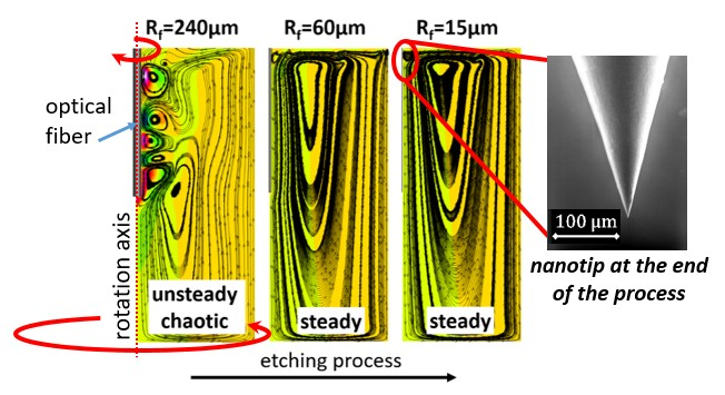
13]). The basic idea is to use rotation movements to generate different kinds of flows inside a vial, which, modifying the shear stresses acting on the fiber due to fluid viscosity and the diffusivity of the system, should allow to control shape and surface characteristics of the obtained nanotip, formed on the fiber inserted into the vial. Results have shown potential in terms of characteristics control.
Figure 1, which derives from a previous work by the same research group [
13], shows the comparison between different regimes of fiber and vial rotation, generically referred to as slow and fast rotation (these generically fast and slow rotation regimes are not to be confused with the TCN1 and TCN2 cases that will be further introduced).
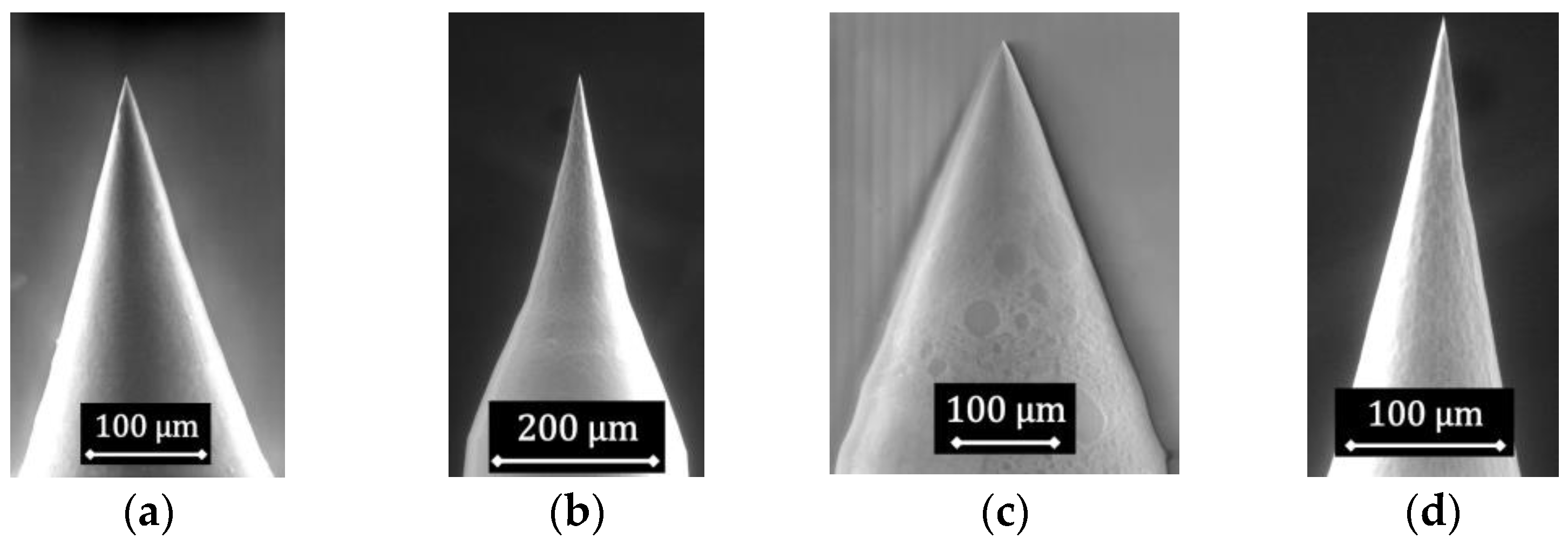
Figure 1a,b show a linear and a curved profile obtained respectively by slow and fast rotation.
Figure 1c,d show the cone angle variation from 50° to 25° obtained respectively for the slow and the fast case. Rotational velocity influences also surface roughness: lower ripples are present in the fast rotation case, with a decrease from 10 nm to 7 nm in the averaged root-mean-square roughness with respect to the slow case.
The present work proposes an extension of the research described in [
13], hereafter referred to as previous work, where the innovative methodology for fibers nanotips production was introduced and a preliminary fluid dynamic analysis of the system performed. The aim is to use Computational Fluid Dynamics (CFD) to improve the knowledge about the fluid dynamic behavior of the mechanical-chemical etching apparatus based on Taylor-Couette systems characterized by unconventional radius ratios with respect to what is found in literature (for the present case, radius ratio and aspect ratio before the etching process are respectively η = 0.0417 and Γ = 1.27). The system is composed of two coaxial and independently rotating cylinders; the internal one is the optical fiber while the external one is the vial. The vial is filled with three stratified fluids: air, oil, and an aqueous solution of hydrofluoric acid (HF). The three stratified fluids with very different physical properties resulted in a big challenge to be managed, particularly because no information of what to expect, in terms of flow structures, length scales and time behavior, was available. The lack of information has been overcome by means of an accurate numerical simulation setup, based on grid sensitivity analysis, time step testing and by means of comparison of the available surface tension models, always having regard of the final objective of the work that consists in the analysis of the obtained flow regimes and their physical characteristics. In the previous work, two different rotational speeds, characteristics of the operating range of the system were selected for the purpose and will be hereafter referred to as test case number 1 (TCN1) for the slow case, and test case number 2 (TCN2) for the fast one. In the present work, some of the main outcomes of the previous work are initially treated in order to make clear to the reader what the starting point of the present research is. A novel analysis of the effects of the mechanical-etching process on the flow characteristics has been then performed in order to evaluate the expected flow regimes representative of the temporal evolution of the process itself. Finally, the flow regimes between the two characteristic rotational speeds previously defined have been explored. The analysis allows the evaluation of the thresholds between different flow types and gives producers the instruments to be able to select a specific regime to be tested and to improve the opportunity to control of the process.
2. Preliminary Analysis
A preliminary analysis of the system has been performed in order to evaluate the expected flow features. Such analysis is in fact necessary to enable adequate selection of the model parameters. For example, the opportunity to select a simplified 2D fluid model instead of a complete 3D one is related to the expected flow regimes. Moreover, the preliminary analysis enables to correctly set up the numerical procedure.
At the beginning of the work, no information was available about the flow regimes that characterize the investigated Taylor-Couette system; therefore, a literature survey has been performed in order to derive some preliminary indications. The geometrical parameters of the proposed system are different from all of the works found, included the works by Andereck et al. [
9] and the more recent ones by Ostilla-Mónico et al. [
15] and Grossman et al. [
10]. In terms of radius ratio, the work by Ostilla-Mónico et al. [
15] is the closest to the present case but Reynolds number values are much higher than the ones relative to our analysis. However, some preliminary considerations have been made. Considering the work of Andereck et al. [
9], the expected HF flow regimes are respectively a Couette flow for TCN1 and a wavy vortex flow or modulated waves for the TCN2 case. Mahamdia et al. [
16] evidenced that, as the aspect ratio decreases, wavy flow generation tends to be disabled. Moreover, the test case is expected to be highly sensitive to top and bottom effects due to its low vial height. In conclusion, since no information about the flow regimes expected have been found for the geometrical parameters similar to the ones of the present model, a complete 3D domain seems to be the more suitable choice for the preliminary analysis, in order to allow capturing the tangential fluctuations if allowed to be triggered. The inner- and outer-cylinder Reynolds numbers, defined for the HF with respect to the tangential velocity and shown in
Table 1, for TCN1 case are respectively—9 and 210 while for the TCN2 case are −880 and 630 with counter-rotating fiber and vial.
3. Description of the Test Case
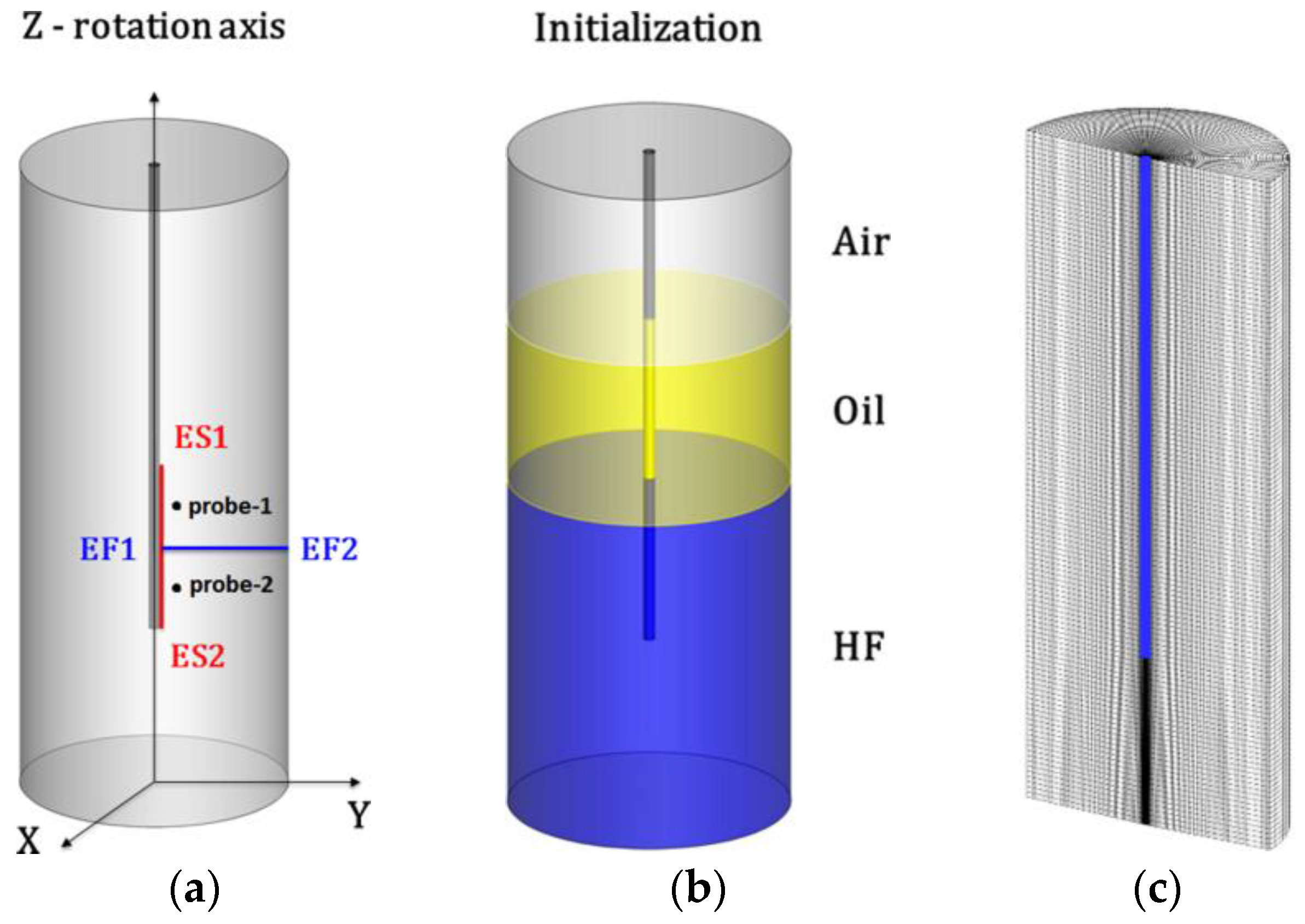
The geometrical model used for the CFD analysis is shown in
Figure 2a,b. As previously stated, it is a 3D closed domain with rotating boundaries that reproduces the experimental setup of [
13]. Half of the vial is filled with an aqueous solution of hydrofluoric acid (HF) which has a density of 970 kg/m
3 and a dynamic viscosity of about 0.00092 Pa·s. A quarter is filled with oil, with a density of 950 kg/m
3 and a dynamic viscosity of about 0.019 Pa·s, with the function of protecting the stem of the fiber from the corrosive HF vapor. The top quarter is filled with air at atmospheric pressure and temperature. The fiber is immersed in the HF for a third of its total height (0.007 m). The radius ratio η between fiber and vial is 0.0417 and the aspect ratio Γ referred to the third of the fiber immersed in HF is 1.27. The height of the vial is 0.028 m while the height of the fiber is 0.021 m. In the TCN1 case, fiber and vial rotate at the same absolute angular velocity of 6.28 rad/s while in the TNC2 case the fiber rotates at 628 rad/s and the vial at 18.85 rad/s. Fiber and vial are always counter-rotating for both cases. The obtained results have been extracted along the line EF1-EF2 for the fluid variables and along the line ES1-ES2 for the fiber stress data, both shown in
Figure 2a. EF1-EF2 is a radial segment positioned axially at half of the portion of the fiber immersed in the HF. ES1-ES2 is an axial segment, positioned on the external radius of the fiber, that covers all the part of the fiber immersed in the HF.
4. Numerical Approach and Model Assessment
Numerical simulations have been carried out with the commercial code ANSYS® Fluent® on a structured grid. Unsteady calculations have been performed with a second-order upwind scheme for the spatial discretization. The Green-Gauss cell-based method has been used for gradients evaluation. The pressure-based solver has been chosen with the segregated algorithm (PISO) for the pressure-velocity coupling and the PRESTO scheme has been selected for the pressure interpolation.
The Volume Of Fluid (VOF) model, specific for stratified/free-surface flows, has been used with the explicit integration scheme and a Courant number of 0.25. The VOF approach is widely used when two or more immiscible fluids are analyzed. Its implementation in ANSYS
® Fluent
® has been successfully validated in real case studies, showing reliable predictions of experimental data (e.g., [
17]). The Compressive Interface Capturing Scheme for Arbitrary Meshes (CICSAM) [
18], which is suitable especially for fluids with a remarkable difference in dynamic viscosity, was used for the volume fraction interpolation.
No turbulent closure models have been chosen due to the low inner- and outer-cylinder Reynolds numbers considered, as discussed previously.
The counter-rotating movement of fiber and vial is obtained by means of moving walls. The tangential velocities corresponding to the rigid motion of fiber and vial along to their axes have been imposed as boundary conditions on the walls, which are treated as no-slip boundaries. Therefore, at the wall, the flow has zero axial and radial velocity, while it is characterized by a tangential velocity component in the absolute frame of reference. Time-dependent wall velocities have been assigned in ANSYS® Fluent® by means of User’s Defined Functions (UDF).
In terms of model assessment, three different levels of simulations with increasing model accuracy have been tested for both swirling cases in order to understand the effects of model characteristics on the results. The base level, referred to as MOD1, does not account for surface tension (ST) and wall adhesion (WA). The second level, referred to as MOD2, accounts only for surface tension via the Continuum Surface Force method (CSF) of Brackbill et al. [
19]. The third one, referred to as MOD3, accounts for both surface tension (via CSF method) and wall adhesion (WA). A value of 0.047 N/m has been set for the surface tension at the HF-oil interface while the static value of the adhesion angle at the fiber has been set at 17° in the HF domain [
20].
Table 1 shows the simulation matrix with geometrical features, operating conditions and selected numerical models. Simulations have been started at rest conditions, with initialization conditions shown in
Figure 2b, and accelerated through a one-second numerical transient to reach the nominal rotational regime.
The time step has been chosen as a fraction of the revolution period of the fiber in the TCN2 case. A preliminary analysis has been initially performed on MOD1 considering three different time steps equal to 1/100, 1/10 and equal to the period itself. No remarkable differences have been detected for the three cases, thus allowing the selection of a time step equal to the fiber revolution period (0.01 s).
It can be underlined that a lower time step has also been selected as a function of the numerical setup, as reported in
Table 1. In fact, in order to decrease the intensity of spurious currents, which are characteristics of the available surface tension models, the time step in tests 03, 04, 05, and 06 has been reduced to 10
−5 s. Good results have been accomplished for model MOD2 almost reaching the suppression of the spurious currents while MOD3 resulted to be yet affected although with a reduced parasitic currents intensity.
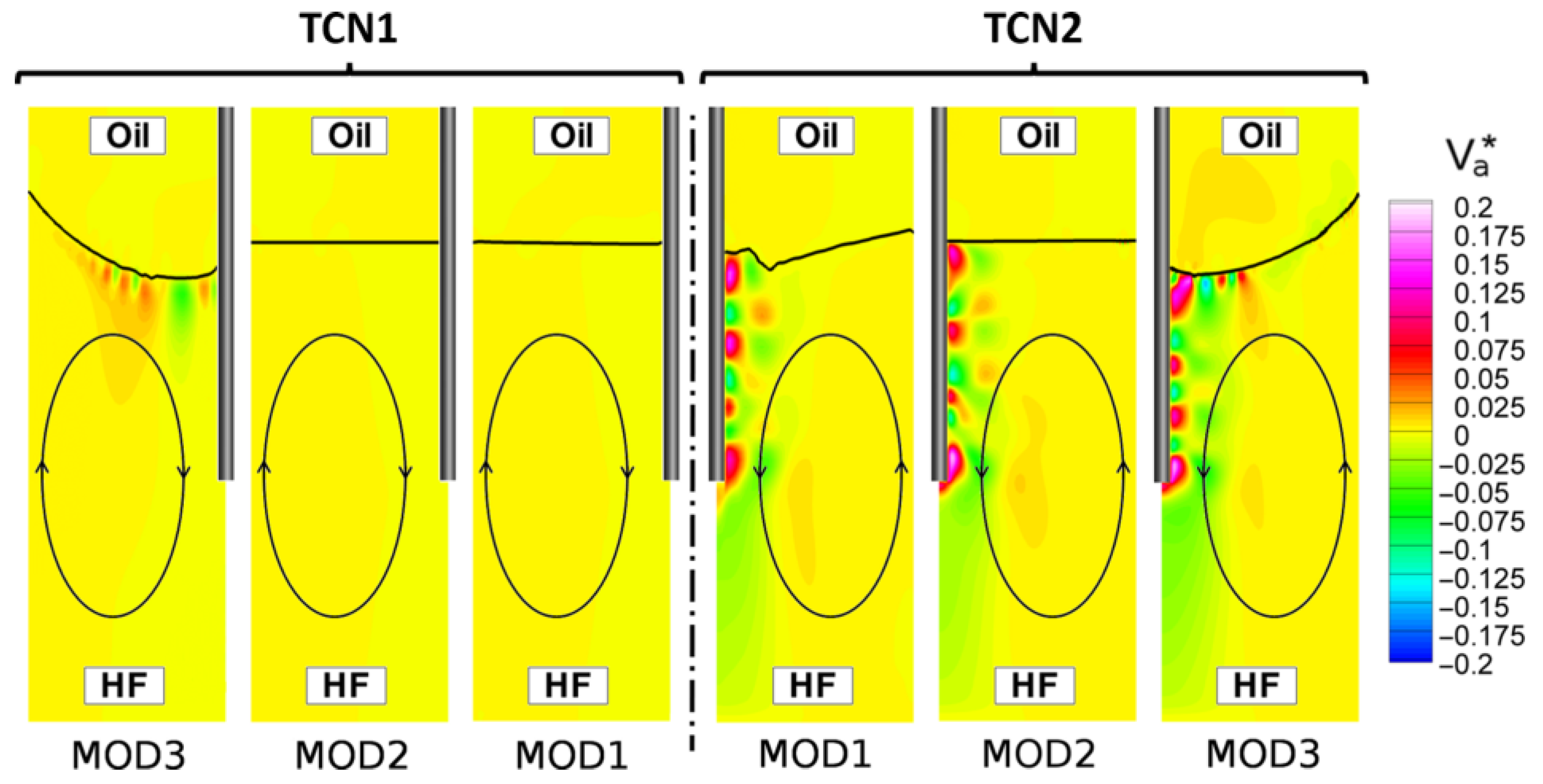
The three models MOD1, MOD2 and MOD3 have been compared in order to evaluate the effects of the increasing accuracy. The comparison, reported in
Figure 3, has shown significant differences in terms of shape of the interface surface, with a more physical reconstruction obtained by model MOD3, and of numerical spurious currents, which in contrast are found in MOD3, the most suffering model. This numerical problem affects the solution in a region confined closely to the fluids interface and its consequences are mainly involving the surface shape. General flow fields seem in fact to be only locally affected by spurious currents.
Although the highlighted differences are quite significant, global results, to be intended as stresses along the fiber and vortical structures, are not affected by the choice of the model. Same qualitative flow conditions are in fact obtained with and without ST and WA models both for TCN1 and TCN2 cases.
In particular, vial driven core flows (highlighted via a black elliptical line in
Figure 3) are evidenced for both the TCN1 and TCN2 conditions, although with a difference in terms of vortex intensity due to the different boundary conditions. These core vortices result to be generated by the so-called Ekman pumping effect, related to the rotation of the bottom end of the vial.
The high-speed case (TCN2) show more complex flow structures superimposed on the mentioned core vortex. In fact, high-intensity vortices are generated closely to the fiber by its rotation. As will be evidenced later such vortices develop in the flow region influenced by the fiber motion that averagely extend for about 20% of the gap between fiber and vial.
In conclusion, except for the effects of the spurious currents and for the shape of the interface, the same differences between the two operating conditions can be evidenced among the three numerical models (MOD1, MOD2, MOD3). In particular, since the analysis intend to focus mainly on flow regimes and on the stresses acting along the part of the fiber immersed in HF, results can be considered independent from the accuracy level of the selected model. However, since MOD1 offers an enormous save of computational time, it has been selected for all of the simulations described further except where a precise positioning of the interface between oil and HF is needed. That is the case of the study of the effects of fiber radius reduction treated in
Section 7.
5. Grid Dependence Analysis
A steady state grid dependence analysis has been performed in order to evaluate the spatial discretization accuracy. Four structured grids have been generated by means of the commercial software ANSYS
® ICEM-CFD
TM. Starting from the coarse grid, referred to as ID1, the other 3 grids have been generated doubling the number of elements axially, radially and tangentially at each step, obtaining the finer grids respectively named ID2, ID3, and ID4. The geometrical model used for the grid dependence analysis is the same previously described but the vial is completely filled with HF and the fiber is long enough to be completely immersed in it, in order to obtain the maximum number of vortices. For the same reason the rotation regime selected for the purpose is TCN2 with its more complex flow features. Results, in terms of non-dimensional fiber torque (that is an aggregate parameter for the evaluation of the stresses acting on the fiber) are shown in
Table 2 together with the main features of the grids.
The optimal grid emerged from the sensitivity analysis is ID3, with its 720892 elements against 5767136 of the ID4. A substantial reduction in terms of computational costs is paid by only a 0.7% difference in the evaluation of the torque acting on the fiber (C
f/C
ref,f) with respect to the finest grid (ID4). The same considerations can be extended to the vial, where a slightly higher value of C
v/C
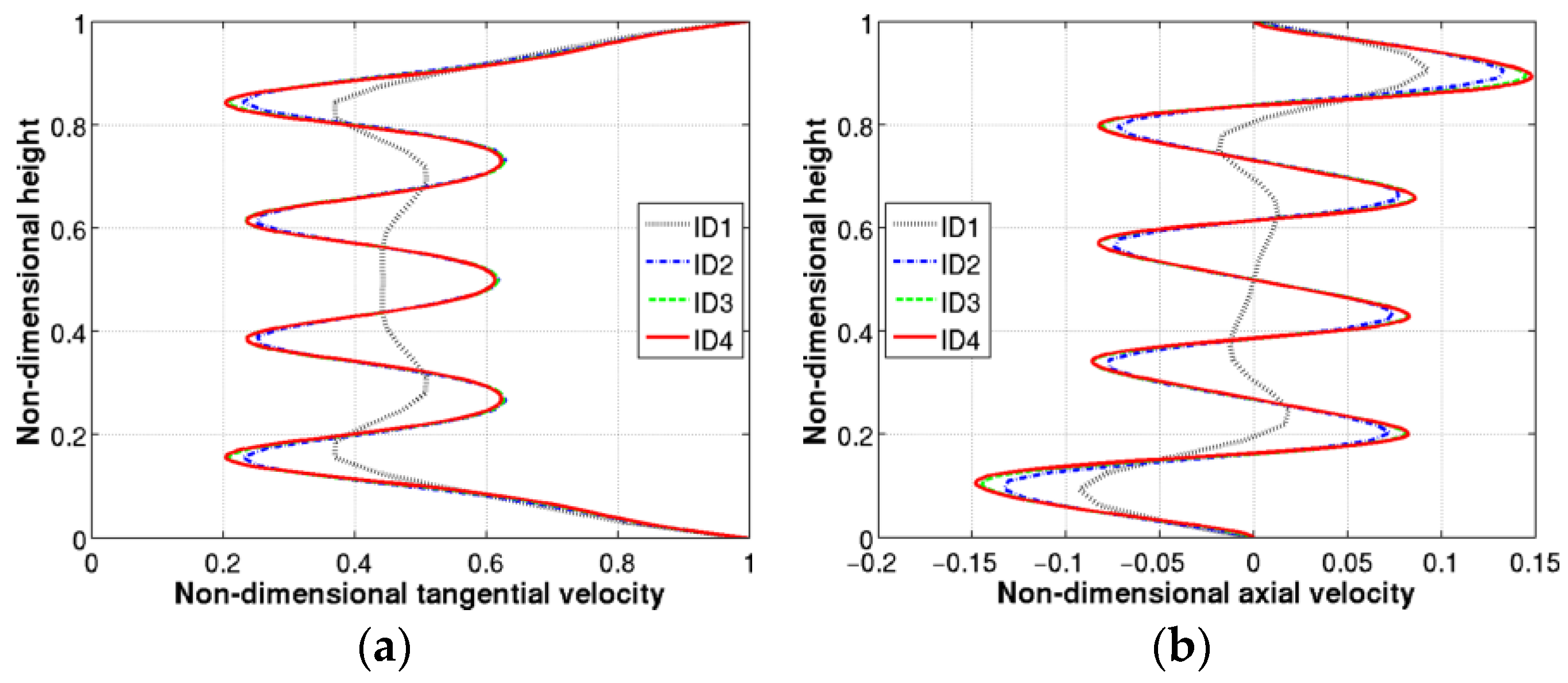
ref,v is obtained. Same accuracy in the reconstruction of vortical structures is also achieved between the two grids ID3 and ID4 as shown in
Figure 4a,b, respectively referred to tangential and axial flow fields. Velocity data used for the grid dependence analysis are extracted along a vertical line in the middle of the gap between fiber and vial. Non-dimensional tangential and axial velocities are defined as V
t/U
ref and V
a/U
ref, being U
ref the tangential velocity of the fiber:
Based on the results of grid sensitivity analysis, the same resolution has been applied to the actual case (
Figure 2a). The obtained grid is shown in
Figure 2c.
6. TCN1 and TCN2 Flow Regimes
A description of the characteristics of the flow regimes relative to TCN1 and TCN2 cases is reported in this section. Results will be shown in terms of non-dimensional values. The reference values for velocities and stresses are respectively the tangential velocity of the fiber U
ref defined in Equation (1) and the tangential stress, obtained in the HF, considering the nominal variation in tangential velocity over the cylinders’ gap:
Both the reference values U
ref and τ
ref have been evaluated for the TCN2 case.
6.1. Time-Dependent Behavior
The first main difference between the two cases is that, after reaching the nominal rotation regimes (i.e., the transient on boundary conditions is over), TCN1 reaches a steady state condition after about 13 s, while TCN2 shows instead an unsteady behavior. Since no periodicity has been found for the TCN2 case, although a long time of numerical data acquisition has been considered, the simulation has been interrupted with the following criterion. The window of acquisition was long enough to obtain representative data of the process but not too long to introduce discrepancies between the geometry of the numerical model and the real fiber geometry during the process. In fact, the fiber shape changes due to the etching procedure and induces a modification of the flow regime as will be described in
Section 7. Since no reproduction of chemical etching of the fiber is considered for the present part of the work, the error in reproducing the fiber geometry increases with time. The limit for such error has been imposed in order to be of the same order of magnitude of the error done on torque evaluation deriving from the selection of the ID3 grid instead of the ID4, which is 0.7% as previously explained.
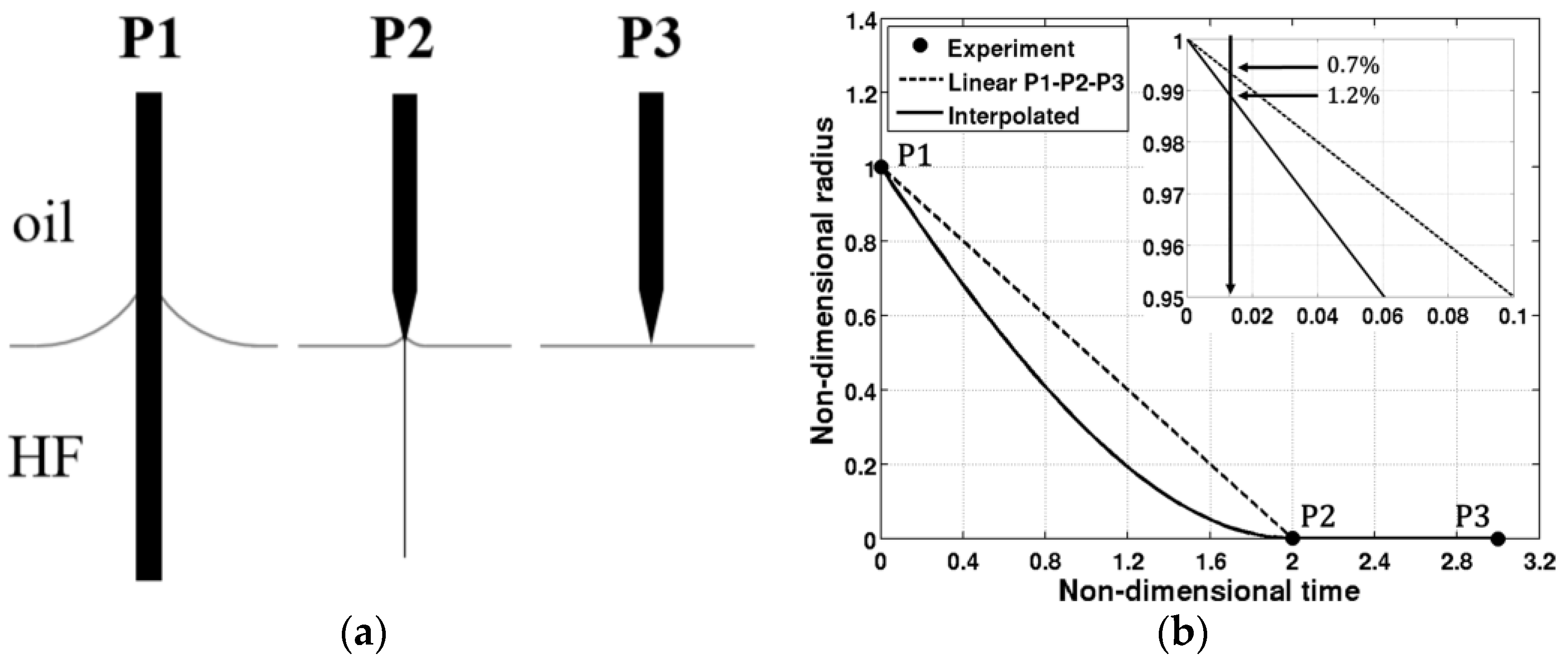
Figure 5a shows schematically the process of formation of the tip which is quantified in
Figure 5b in terms of non-dimensional quantities. Non-dimensional radius is defined as the ratio between the actual fiber radius relative to the part immersed in the HF and the radius of the intact fiber. Non-dimensional time is defined as t/t
ref with t
ref equal to one hour. Two curves based on the available experimental data aim to represent this mechanical-chemical etching process. Only two experimental points are available. Point P2 in
Figure 5 when the fiber is almost completely etched and point P3 in the same figure that represents the end of the process. This allows two different available reconstructions of the etching process, as shown in
Figure 5.
For the first evaluation, mechanical-chemical etching process is approximated via two linear etching rates: a faster one from P1 to P2 and a slower one from P2 to P3. The second evaluation is obtained by means of quadratic interpolation represented by the curve connecting points P1, P2, and P3. In the authors’ opinion, the most physical behavior is represented by the interpolated curve whose shape account for different etching rates related to the variation of dynamical diffusivity and acid concentration. Anyhow, having no information about the actual path between points P1 and P2, a conservative choice has been done and the linear P1-P2-P3 line has been used as a reference. Thus, maintaining the geometrical error lower than 0.7% implies that 47 seconds of simulation give a coherent superior time bound for TCN2 (with this temporal window, the interpolated line would induce a 1.2% geometrical error).
6.2. Zones of Influence of Fiber and Vial
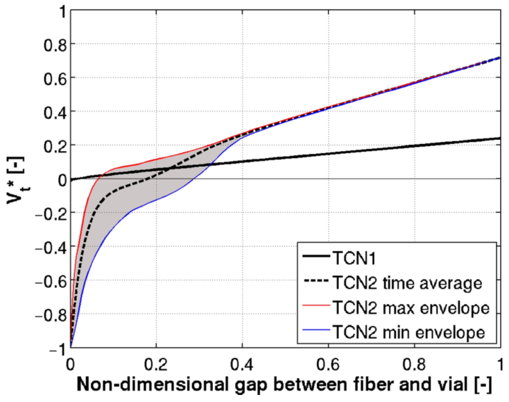
The evaluation of tangential velocity fields along the line EF1-EF2 in
Figure 2a allows an estimation of the influence areas of fiber and vial (i.e., the zones where rotation of one boundary is dominant with respect to the other). Such influence areas can be defined respectively as the ones where local tangential velocity is concordant with wall rotation.
Figure 6 compares the two reference operating conditions in terms of non-dimensional tangential velocity. Since TCN2 is unsteady, a time average value is reported together with the envelope curves of the maximum and minimum values.
It is evident that, under TCN1 conditions, the area of influence of the fiber is almost negligible and hence the fluid is completely driven by the vial, resulting in the rotating core flow previously cited. TCN2 instead shows an area from about 6% up to 29% (averagely 18%) of the gap between fiber and vial where the flow is driven by the high swirling velocity of the fiber.
6.3. Vortices Configurations
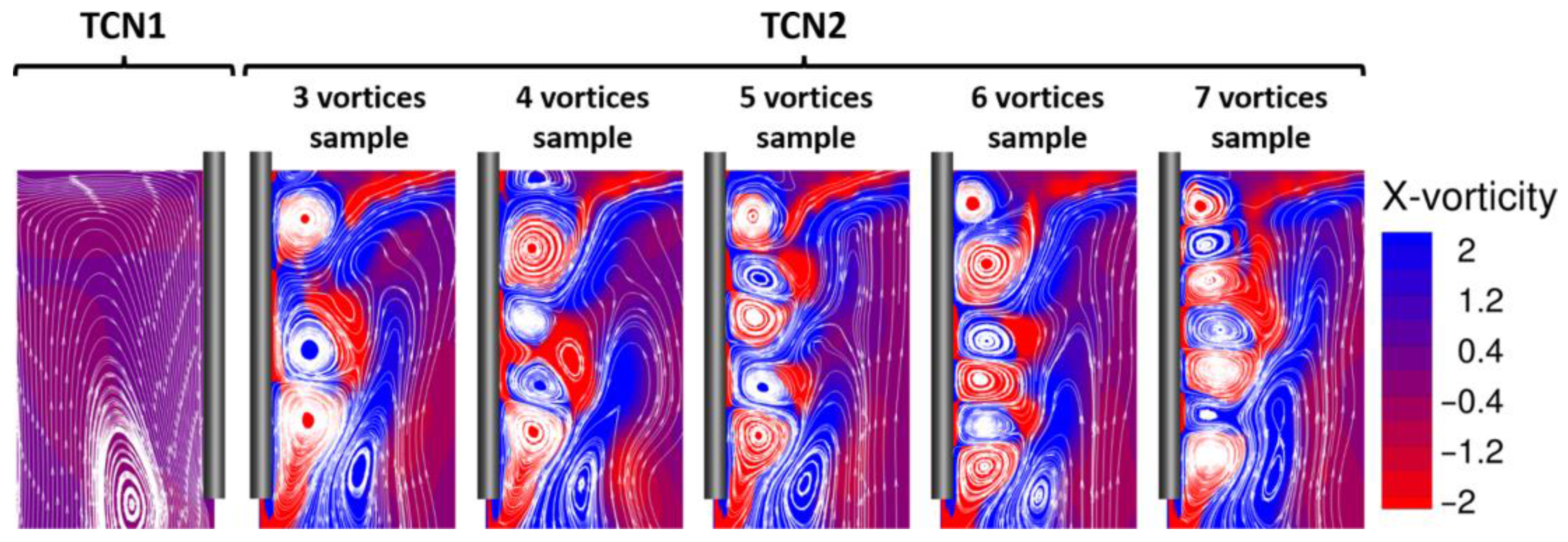
Figure 7 shows the vortical structures characteristic of the two reference configurations. For an easy individuation of the vortices, streamlines, highlighted in white, are superimposed on the contours of
X-axis vorticity. The steady core flow of TCN1 is shown on the left of
Figure 7. In contrast, the flow structure of TCN2 is highly unstable. Vortices are continuously and chaotically generated during the evolution of the flow and five typical configurations have been individuated. A different number of vortices adjacent to the fiber, ranging from three to seven, characterizes such configurations, and samples thereof are reported in the right part of
Figure 7.
TCN1 case is substantially a vortical core driven by Ekman pumping effect related to the vial rotation. Instead, TCN2 case has aggressive vortices generated by the centrifugal action of the swirling fiber. These vortices interact with the fiber and the core flow driven by the vial.
It has also been observed that when the number of vortices is odd the vertical structure is more stable, especially the five-vortices configuration, while even ones have a shorter life due to their intrinsic instability. Configurations with an even number of vortices are in fact characterized by co-rotating vortices interactions that provides suppression (or merging) of the weaker ones.
It has been experimentally demonstrated that rotational regimes are correlated with the nanotips shapes. As evidenced above, the two tested operating conditions correspond to very different flow regimes with remarkable differences in shear stress intensity and flow structures. Since mechanical-chemical etching is influenced by these latter characteristics, it is possible to conclude that the different shapes obtained can be directly linked to the flow regime generated inside the vial.
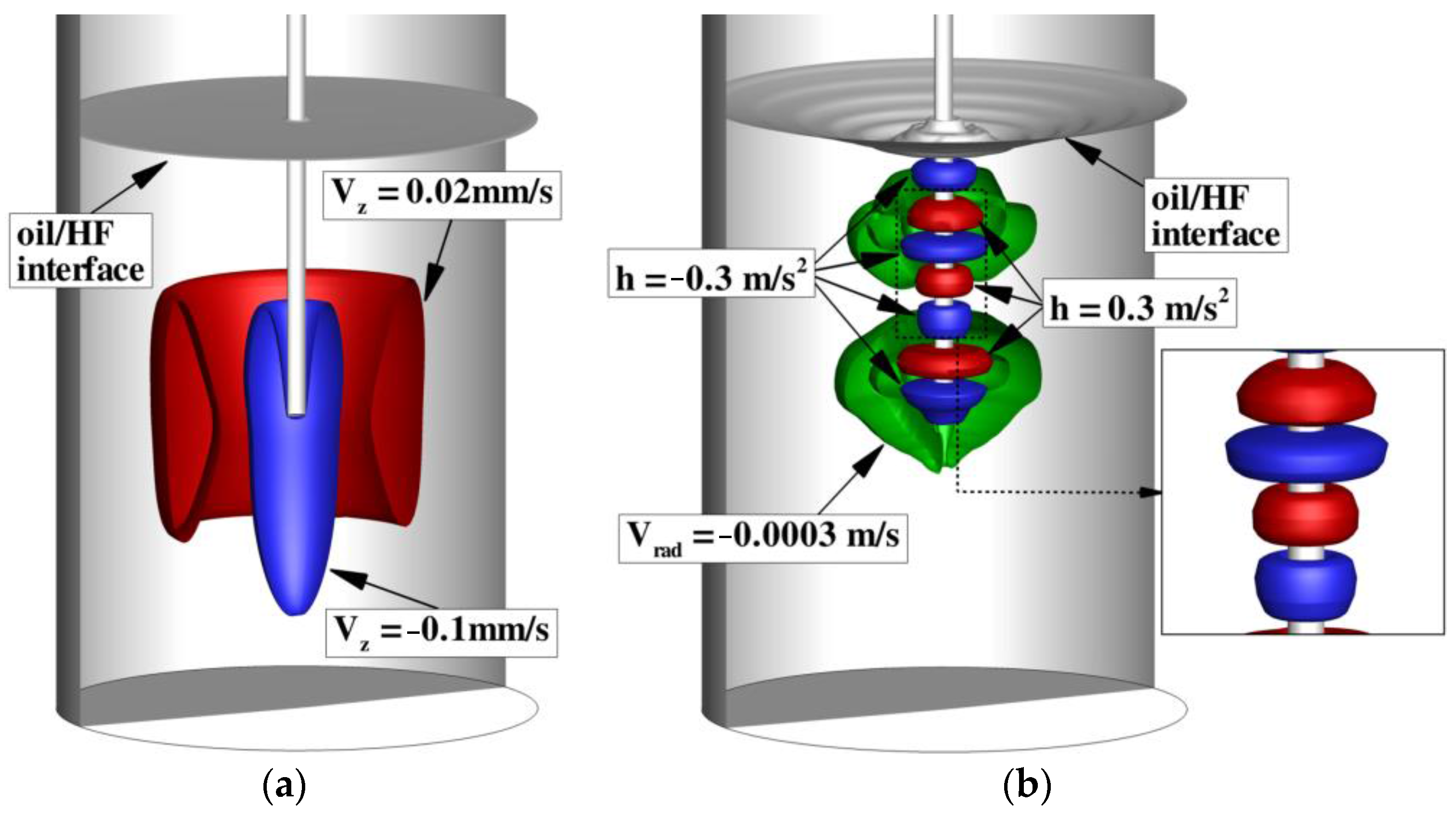
It is worth underlining that the flow structures observed for TCN1 and TCN2 are axisymmetric. A representation of such axial symmetry is provided in
Figure 8, where a section of the lower half of the analyzed Taylor-Couette system is reported. The section shown is extended from the bottom of the vial to about half of the oil layer (i.e., about 0.003 m above the HF-Oil interface). For the TCN1 case, the axial symmetry is represented through isosurfaces of constant axial velocity. For the TCN2 case, a generic instantaneous 7-vortices configuration (different from the one reported in
Figure 7) is presented. The symmetry of the vortical structures is evidenced through isosurfaces of constant helicity density (
h). Helicity density is defined as the scalar product between the local velocity and the vorticity vector:
A positive helicity density shows a vortical structure characterized by the projection of the vorticity vector along the local flow velocity direction having the same orientation of the velocity field itself. The alternation of vorticity direction clearly appears from
Figure 8b.
6.4. Shear Stresses Along the Fiber Surface
Tangential and axial shear stresses along the fiber surface have been evaluated and compared for TCN1 and TCN2. Stress data are extracted along the ES1-ES2 line shown in
Figure 2a. ES1 corresponds to the position of the meniscus that generates the nanotip. Non-dimensional tangential shear stress is about −0.7 for the TCN1, while TCN2 has an average value of −46, with a maximum of −175 and a minimum of −28, thus two to three orders of magnitude difference are present between the two cases in terms of tangential stresses.
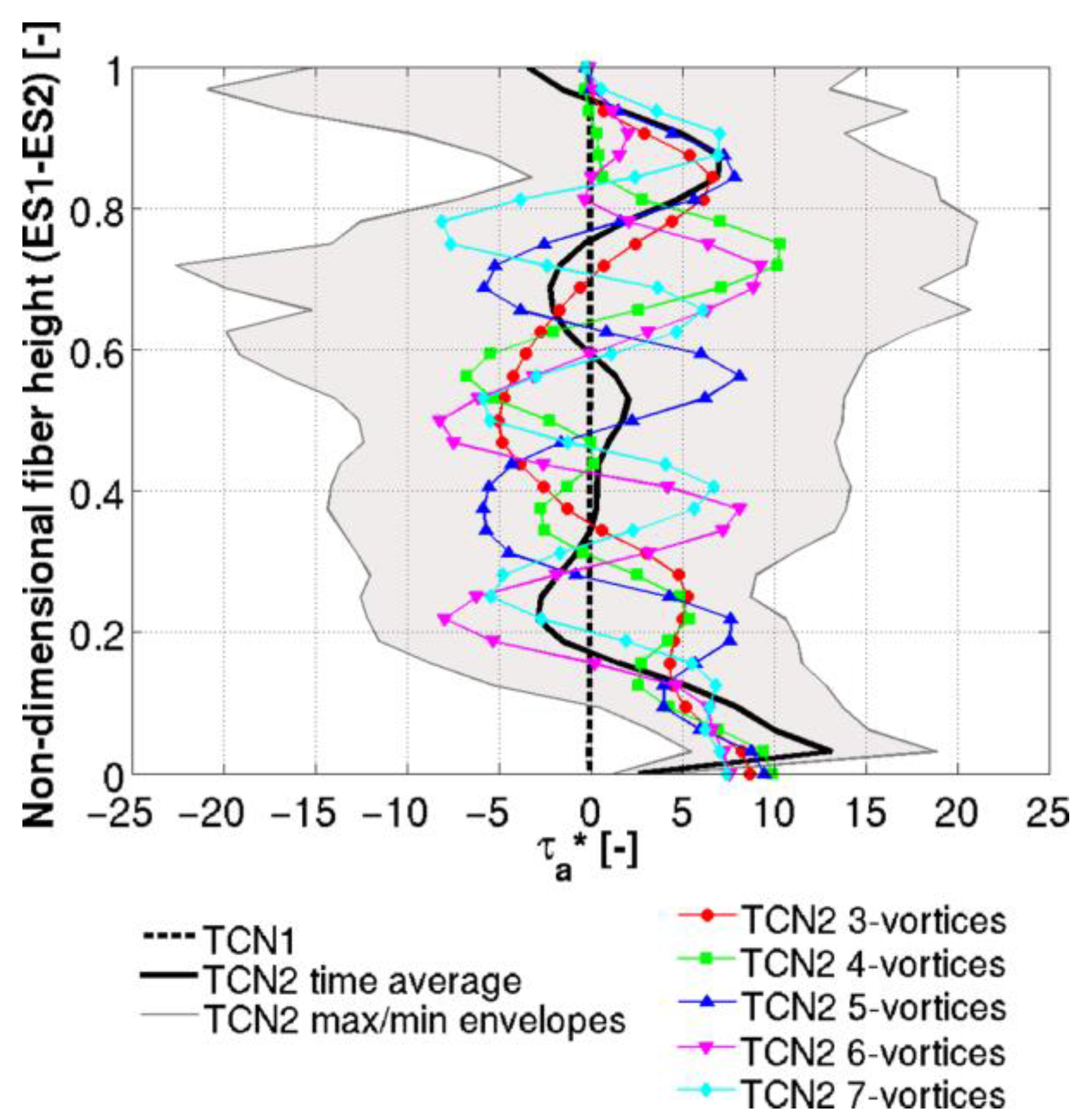
Figure 9 reports a synoptic presentation of the axial shear stresses acting on the fiber skin. Again, orders of magnitude are completely different: TCN1 is characterized by a steady-state non-dimensional axial shear stress of about −0.005 while the time average value for TCN2 ranges from −25 to −23. The solid black line of
Figure 9, that represents the time average axial stress for TCN2, shows a structure of five vortices that resulted to be the more stable and more frequent condition in the TCN2 chaotic motion. Such remarkable difference in terms of stresses, acting contemporarily with the etching process, could be responsible to play a major role in determining the production time of the nanotips. In fact, experimental tests evidenced that the fast case resulted in a lower production time (about −20%) with respect to the slow case, highlighting the role of shear stresses on the mechanical-chemical etching process. The lack of accuracy of the model in providing the meniscus shape and the absence of chemical etching in the model do not allow drawing conclusions about the consequence that such different characteristic shear stresses have on the nanotip shape.
The colored curves of
Figure 9 show the axial shear stresses for the TCN2 case corresponding to the samples of vortices configurations showed in
Figure 7. The gray band reported, which contain all the other curves, corresponds to the envelope of maxima and minima for the TCN2 case. The instantaneous axial stresses acting on the fiber for all of the vortex configurations oscillate around the averaged value as expected. The main difference is highlighted at the lower end of the immersed fiber, where the time average value, ranging from 0 to 5, is lower than all the instantaneous samples reported, that are between 7 and 10. This apparent incoherence is due to the mechanism that drives vortices formation. Vortices are mainly generated in correspondence of the lower fiber end with ascendant axial shear stress but, during the transition phases between the various configurations reported in
Figure 7, a descendant axial shear stress can be produced.
Finally, since none of the cases touch an envelope curve, it is reasonable to state that the maximum and minimum values of shear stresses are reached during the transition phases between the various vortices configurations reported.
7. Variation of Flow Regimes for TCN1 and TCN2 Due to Fiber Etching
During the nanotip production process, HF chemically attacks the fiber surface in combination with the action of tangential and axial shear stresses induced by the flow. Consequently, a certain etching rate is obtained and the fiber is gradually consumed until the nanotip is created at the end of the process. Therefore, the key non-dimensional geometrical parameters (radius ratio and aspect ratio), as well as Re
i and Re
o, changes during the etching process due to the variation of fiber radius. Since Taylor-Couette systems are very sensitive to the aforementioned parameters, a variation of the flow regimes is expected. For the investigation of such phenomenon, the operating conditions TCN1 and TCN2 have been analyzed considering two different phases of the manufacturing process, after the start of the etching process. Flow regimes individuated in
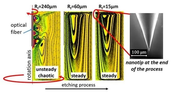
Section 6 allowed the use of two-dimensional simulations due to the absence of azimuthal non-uniformities. Two etched fibers having radius of 60 μm and 15 μm, respectively equal to 1/4 and 1/16 of the radius of the intact fiber (240 μm), have been considered for the analysis. Two new two-dimensional computational grids, with the same resolution described before, have been generated considering the radius reduction for the part of the fiber immersed in HF. Above of the oil/HF interface position the fiber radius has been kept unaltered. In addition to the reduction of the fiber radius, also a reduction of fiber height has been considered at its bottom end of the same amount of radial reduction. The part of the fiber immersed in HF is cylindrical and is connected with the upper part (immersed in air and oil) through a truncated cone which opening angle is imposed to be 40° for the TCN1 case and 25° for the TCN2 case (
Table 3). The truncated cone divides the etched part of the fiber (immersed in HF) from the intact part and is located in correspondence of the nominal oil/HF interface. Time resolved simulations have been performed on the new geometrical configurations using the MOD2 approach for considering the effect of surface tension in maintaining the interface position and taking advantage from the higher time step allowed. Simulations were started from initialization conditions of
Figure 2b and considering a time interval long enough to obtain a fully developed flow regime. It is worth underlining that no chemical process is modeled but etching is reproduced simply by means of a reduction of radius of the fiber geometry between the simulations.
The variation of non-dimensional parameters due to fiber etching is reported in
Table 3. Due to their definitions, aspect ratio and outer Reynolds number undergo limited relative changes with respect to the values calculated in case of intact fiber. In contrast, radius ratio and inner Reynolds number are strongly modified by the reduction of fiber radius for both TCN1 and TCN2. Considering that a reduction of the Reynolds number bring to a reduction of the possibility of insurgence of unsteady effects, it is possible to expect that TCN2 is subjected to the most intense flow structure variation. In support of such consideration, it should also be considered that the unsteady structures of TCN2 are located in the area of influence of the fiber, which is associated to the most relevant change in Reynolds number. Unfortunately, the new non-dimensional characteristic parameters do not match any literature work in authors’ knowledge.
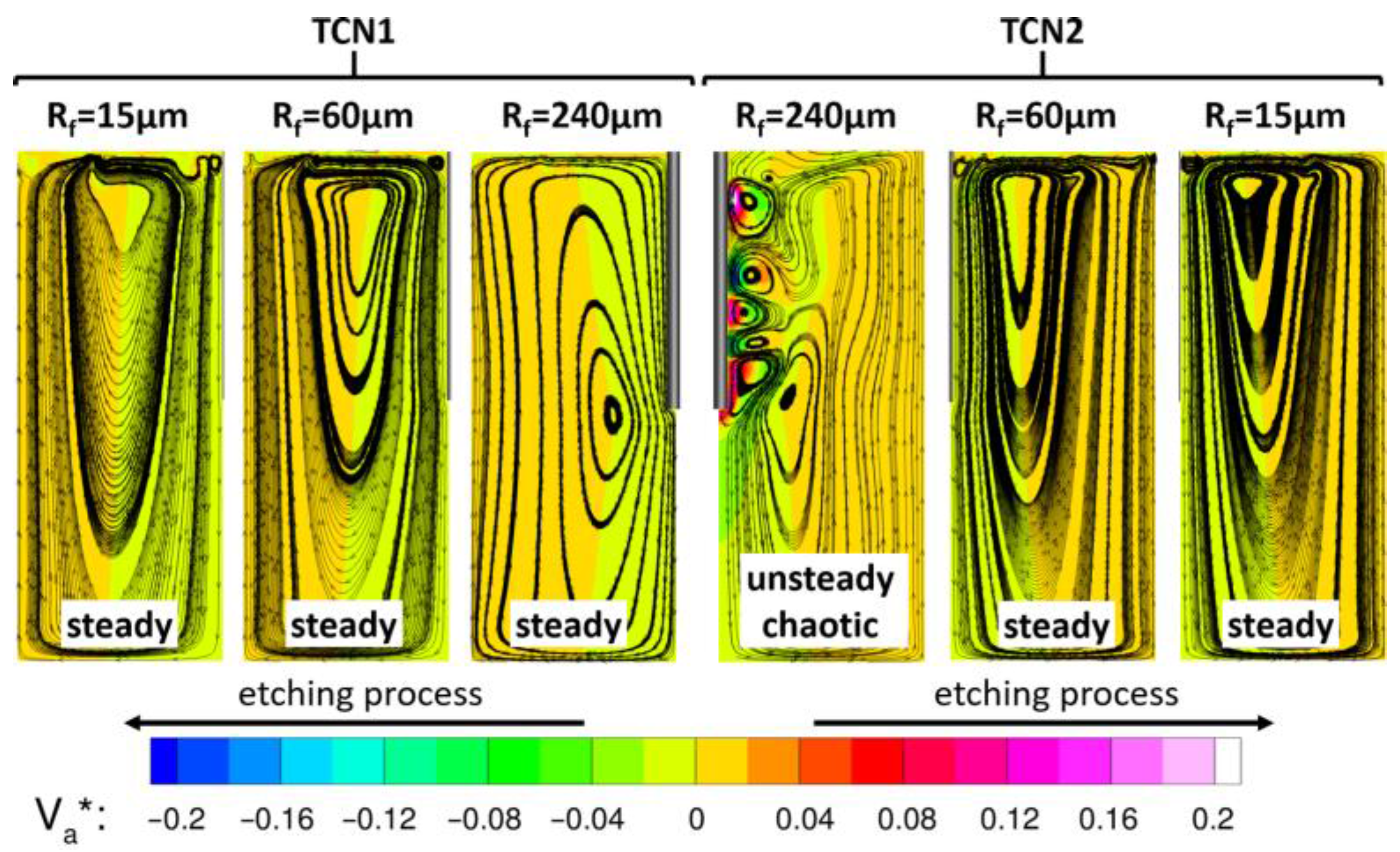
Figure 10 reports the flow structures that characterize the various phases of the etching process for TCN1 and TCN2 operating conditions. As it is possible to observe, for the TCN1 case, all the investigated fiber radii generate a steady flow field. TCN2 undergoes a transition phase from unsteady chaotic to steady motion passing from the intact fiber to a radius of 60 μm and remains steady for 15 μm. For both TCN1 and TCN2, the core vortex located initially about in correspondence of the height of the bottom end of the fiber, moves upwards with the reduction of the fiber radius.
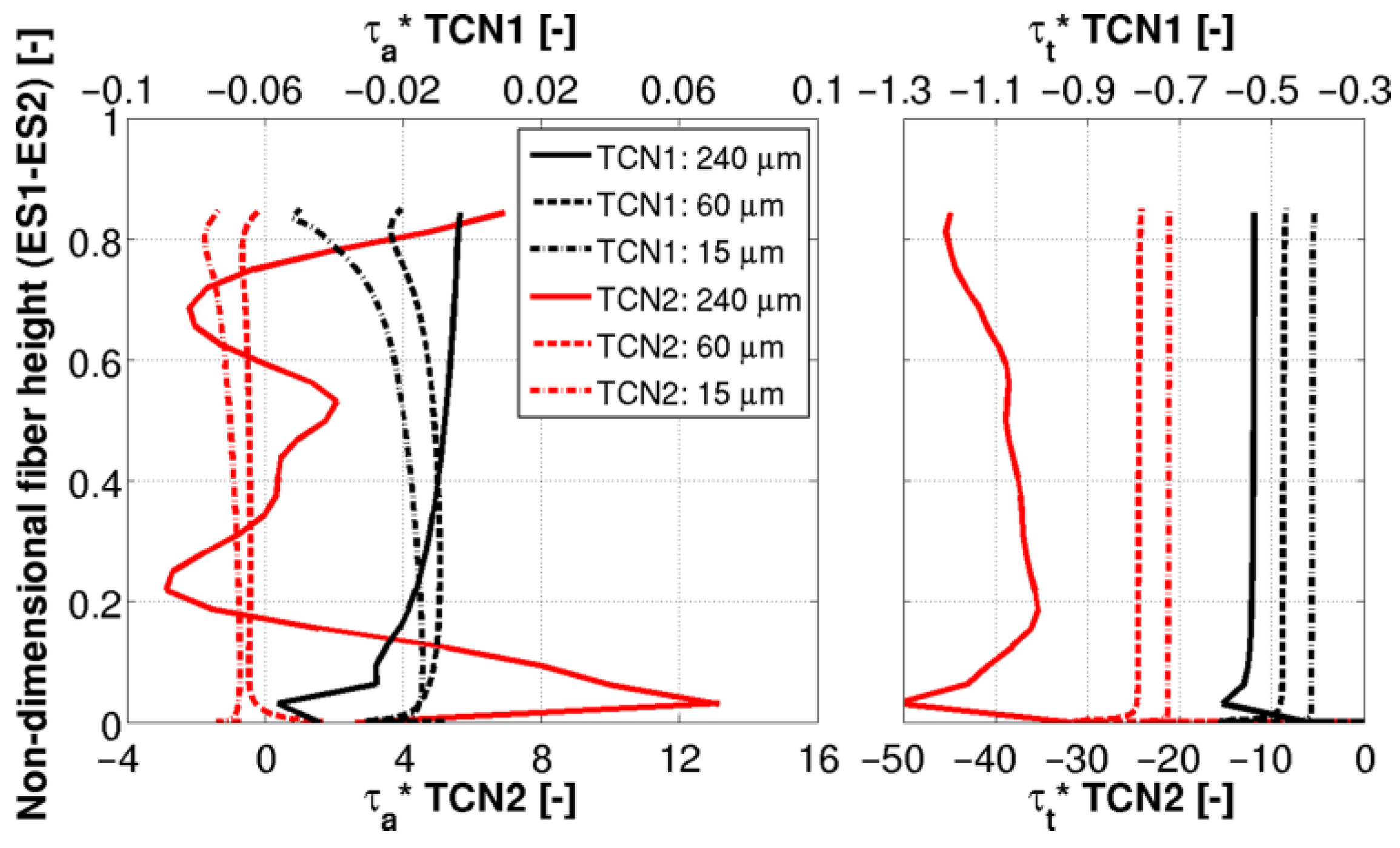
The modification of flow regime encountered during the etching process generates variations of the shear stresses along the fiber surface, which in turn influence the etching rate. The distributions of non-dimensional axial and tangential shear stresses along the part of the fiber immerged in HF (ES1-ES2 line of
Figure 2a) are reported in
Figure 11. Shear stresses relative to TCN1 are significantly lower than the one associated with TCN2 both for intact and etched fiber. Except the axial pressure gradient due to gravity (equal in the two cases), there are no other external axial pressure gradients acting on the system that can induce torque reductions [
21]. Differences on shear stresses are only ascribable to the different rotation regimes.
Looking at the tangential stress (right part of
Figure 11), a monotone reduction of its magnitude can be observed with radius reduction for both TCN1 and TCN2 but this latter is characterized by a stronger relative reduction passing from 240 μm to 60 μm due to the aforementioned regime transition. Considering axial shear stresses (left part of
Figure 11), interesting behaviors can be highlighted for both the operating conditions. For the TCN1 case, consequently to the upward movement of the core vortex commented before (see
Figure 10), the high-stress zone located at the bottom end of the intact fiber moves upward when the fiber radius is reduced. For the TCN2 case, due to the suppression of vortical structures close to the fiber, the spatial fluctuation of the average axial shear stress disappear passing from 240 μm to 60 μm. Moreover, although the dominant component of stress is the tangential one, for both TCN1 and TCN2, the absolute value of axial shear stress increases passing from 60 μm to 15 μm. Such behavior could be ascribed to the aforementioned upward movement of the core vortex that implies stronger radial gradients of axial velocity in the upper part of the HF.
8. Flow Regimes Obtainable Through Variation of Rotational Speeds of Fiber and Vial between TCN1 and TCN2
This section proposes an in-depth analysis of the flow regimes characterizing the system when different inner and outer rotational speeds are imposed. Such an analysis is mainly directed to fiber producers and allows highlighting the operating ranges to be used for a better control of the process.
The range of rotational speeds explored in this work is selected by means of a linear variation between the two reference cases, i.e., TCN1 and TCN2. Such a choice, together with the choice of maintaining constant fiber and vial’s acceleration, thus varying the transient time necessary to reach regime motion, has been considered in accordance with current trends in fiber nanotips production. Results presented in this section have been obtained using the MOD1 configuration and, as for
Section 7, by means of two-dimensional simulations.
The bisection method has been used to identify the expected thresholds between the different flow regimes observed. The threshold identification has been retained completed when the relative change in terms of fiber’s rotational speed is below 3% with respect to its local value. Such a procedure entailed 45 simulations to be carried out in order to scan the whole selected range. Operating parameters of the simulations are reported in
Table 4.
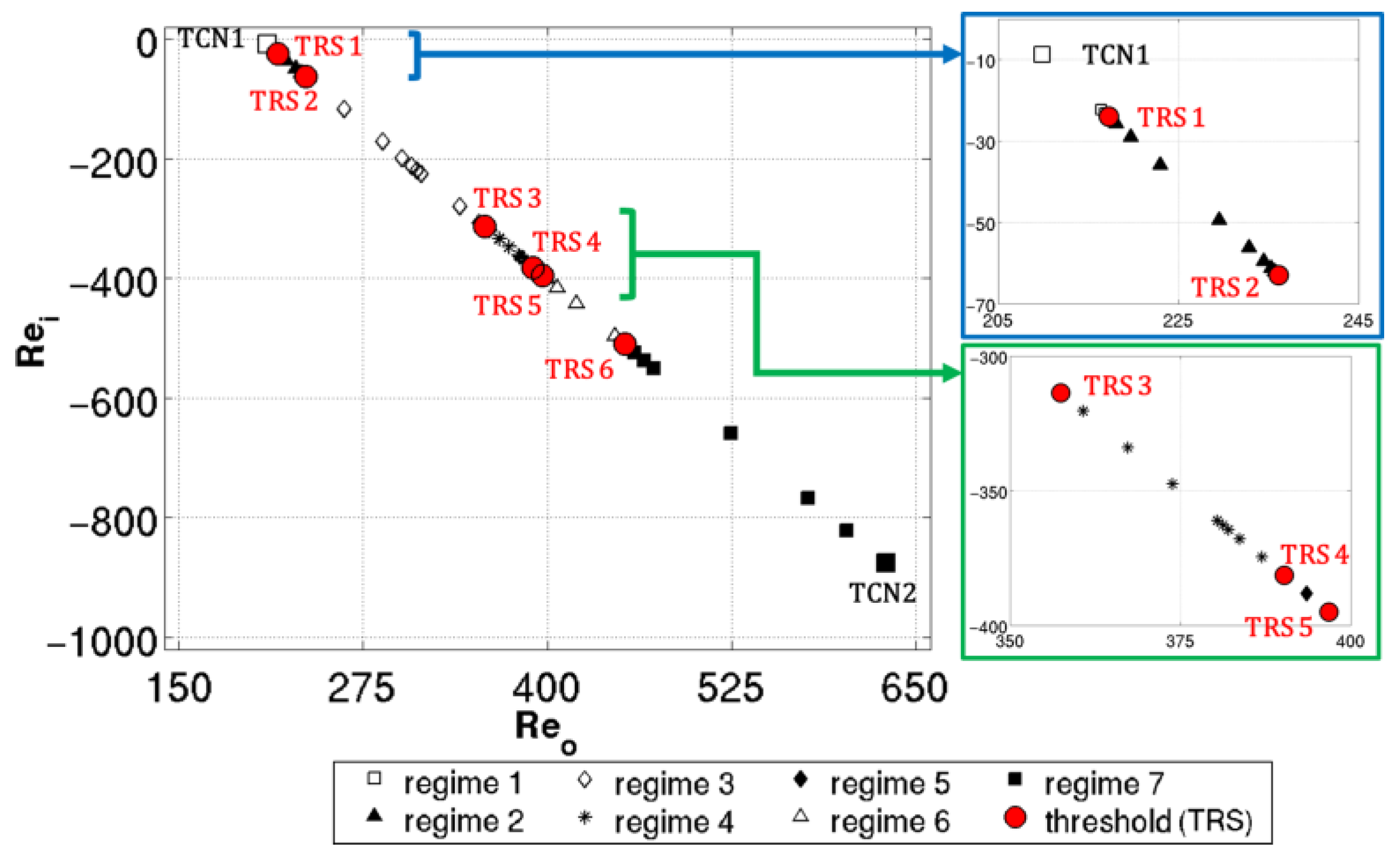
Figure 12 and
Figure 13 show the results of the proposed analysis. In particular,
Figure 12 shows the tested points in a Re
i – Re
o plane, highlighting six thresholds (TRSs) separating seven characteristic flow regimes, including the reference ones (i.e., the extremes points of the explored field).
Figure 13 shows the non-dimensional axial velocity field with superimposed streamlines representative of each of the evidenced classes of flow features.
As proposed in the analysis of the reference regimes the first characteristic to be evidenced is the time-dependent behavior. Between TCN1 and TRS4 (Re
i = −381, Re
o = 390) all of the simulations, after reaching the nominal rotation regimes, obtained a steady state condition. In contrast, above the previously cited threshold (from TRS4 to TCN2), unsteady conditions are highlighted, with both chaotic and periodic behavior. This latter occurs between TRS5 and TRS6 and could be of particular interest for producers since its cyclic nature could allow a better control of the tip formation, at least in the first part of the mechanical-chemical etching process, and the consequent reduction of uncertainty of the produced fibers. Due to the mentioned opportunity, particular focus will be given to periodic cases in
Section 8.1.
About the flow structures, shown in
Figure 13, it is possible to observe an increasing number of vortices in the fiber’s influence area moving from regime 1, that is representative of TCN1 kind of flows, to regime 7, representative of TCN2 kind of flows. This was obviously expected considering the characteristics of the reference cases previously detailed.
In particular, when TRS1 is overtaken, a very small vortex at the bottom of the fiber is induced maintaining the core vortex typical of regime 1. After a further slight increase of rotational speeds, two vortices are generated: one at the interface between oil and HF and the other at the bottom end of the fiber. The first two thresholds results are close to the TCN1 case while the two-vortices configuration is maintained along a larger Reynolds extension up to TRS3 (Rei = −314, Reo = 357). Overtaking TRS3, an additional vortex is induced at about 1/3 of the length of the fiber immersed in HF from its bottom end. All of the highlighted vortices are counter-rotating with respect to the core vortex.
A further increase of rotational speed drives the system across TRS4 thus in the region of unsteady flow types. The first flow type encountered is an unsteady chaotic motion switching from a three- to four-vortices configuration, with all of the vortices yet counter-rotating with respect to the core one. Since TRS4 and TRS5 are very close, only one test highlighted the existence of such a flow type due to the selected convergence criterion of the bisection method. Moving towards faster regimes, above TRS5, the periodic unsteady field is explored. The time-dependent behavior (i.e., periodic versus chaotic) is not the only difference among flows across TRS5: above the threshold and up to TCN2 case both counter-rotating and co-rotating vortices are produced in the influence area of the fiber while only counter-rotating vortices are produced below. The periodic zone, i.e. regime 6, is the third more extended region in the explored range after respectively regime 7 (TCN2 kind of flows) and regime 3 (two- vortices steady configuration). It extends from TRS5 (Rei = −395, Reo = 397) to TRS6 (Rei = −510, Reo = 453) and has been investigated by means of 4 tests that will be detailed in the next section. Finally, above TRS6 all of the flows evidenced a chaotic unsteady behavior similar to the TCN2 case. All of these TCN2 kinds of flows showed an increasing vortices number and intensity moving from TRS6 to the TCN2 extreme.
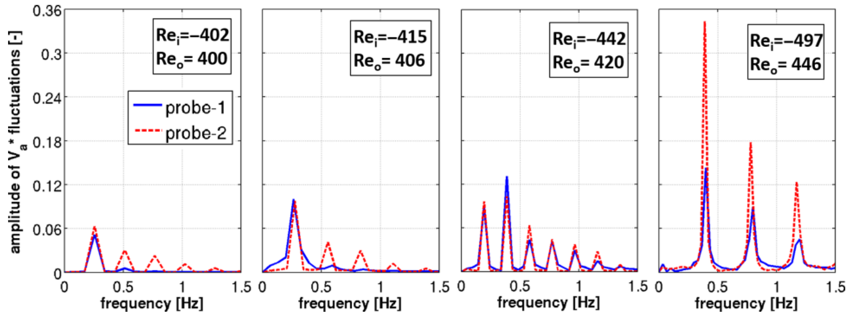
8.1. Details of the Periodic Cases
As previously stated, between TRS5 and TRS6 simulations show an unsteady periodic behavior. The four tests representative of such a behavior have been analyzed by means of the Fast Fourier Transform (FFT) of the non-dimensional axial velocity fluctuations and by means of visual observation of the cyclic flow structures formation and interaction. The signal analysis has been conducted with respect to the data extracted in two points, referred to as probe-1 and probe-2 in
Figure 2a, immersed in the fiber’s influence region. Probe-1 and probe-2 are positioned at a radial coordinate equal to twice the radius of the intact fiber. Probe-1 is located axially 0.00175 m below the oil/HF interface while probe-2 is 0.00175 m above the bottom end of the intact fiber. Results are shown in
Figure 14 for all of the four tests respectively referred to their inner and outer Reynolds values. It is possible to observe that the periodic behavior is obtained when similar absolute values of inner and outer Reynolds numbers are encountered. Moreover, the amplitude of fluctuations increases from lower Reynolds values towards larger due to the increase in intensity of the co- and counter-rotating vortices adjacent to the fiber. In contrast, no correlation has been found among the rotational speed increase and the extension of the period. In fact, moving from left to right in
Figure 14, rotational speed increases while period is respectively of about 3.9 s, 4 s, 5 s and 2.5 s. A slight difference is highlighted among the two probes peak frequencies for the test with Re
i = −415 and Re
o = 406 where a 4s period is given by probe-1 and a 3.6 s long period is found for probe-2.
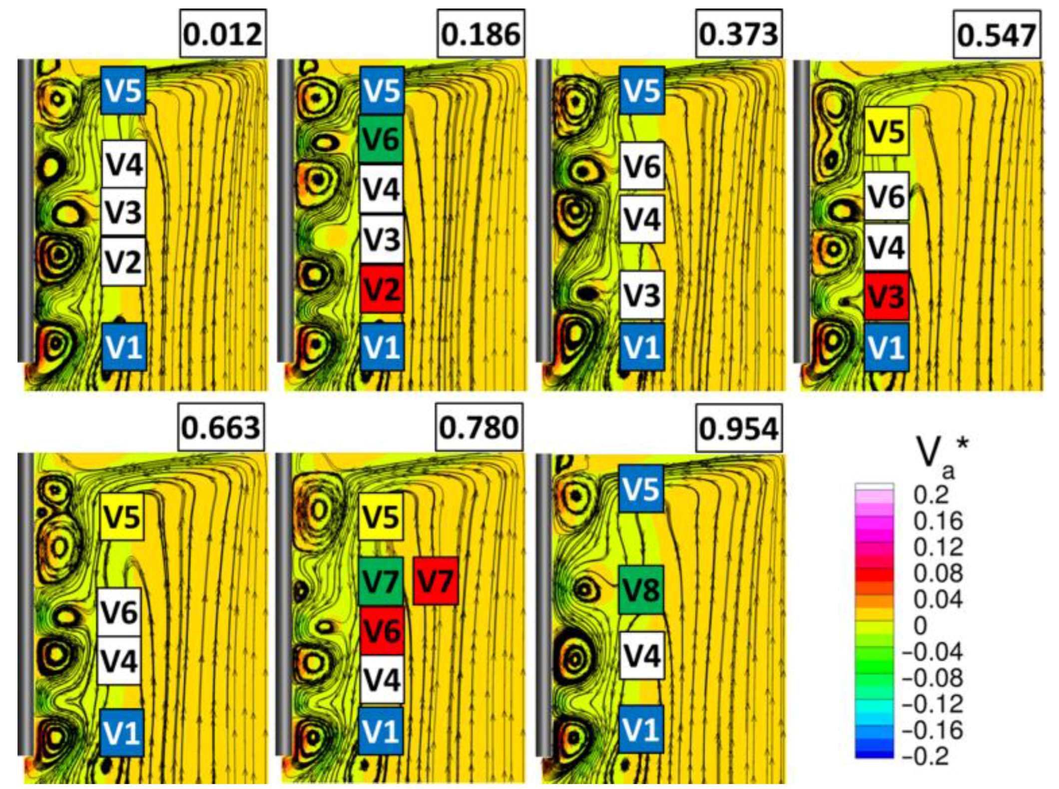
Details of the flow structures of the simulation related to Re
i = −442 and Re
o = 420 are shown in
Figure 15. The case has been selected since it induces the lowest frequency among all of the evaluated cases (i.e., maximum period and number of harmonics). The complex cyclic flow structures highlighted are referred to the non-dimensional period, where the reference one is calculated on the lowest obtained frequency. Vortex 1 (V1) and V5, respectively located at the bottom end of the fiber and at the oil-HF interface, show a slight pulsating behavior in terms of axial extension but substantially remains unchanged through the whole period (blue background color). This description perfectly fits V1 while V5, from 54.7% to 78% of the period, shows a not successful attempt of splitting, with the inception of a very small vortex that is immediately suppressed (yellow background color).
Considering the vortices between V1 and V5, the common trend is a downward movement (white background color), this drives the suppression of V2 and the generation of V6 at 18.6% of the period (respectively highlighted with red and green background colors). The descent of the vortices continues inducing the suppression of V3 and driving the opportunity for V5 to extend, as previously described. When V5 retracts (78% of the non-dimensional period), V7 is generated and acts in the way of suppress and be suppressed by V6. The space left by the mutual suppression of V6 and V7 induces the generation of V8. Finally, V4 and V8 move downward at 95.4% of the period entailing the birth of what was referred to as V4 at the beginning of the process.
9. Conclusions
A numerical campaign has been performed in order to asses and evaluate the fluid dynamics of the innovative setup used for the mechanical-chemical etching process for the fabrication of optical nanoprobes with geometrical and operational parameters different from all the other cases found in literature. Due to a lack of experimental data for the specific case, to be used for validation, particular attention has been given to the reliability of the numerical simulations.
Initially, two characteristics operating conditions (TCN1 and TCN2) have been compared for this purpose. Then, the effects of fiber etching and variation of inner and outer rotational speeds on flow structures have been investigated.
A steady grid dependence analysis has been previously accomplished in order to select an accurate discretization level for the geometrical model. Then, three different models with increasing accuracy and consequently increased computational cost have been tested. Except for the interface surface shape and for the spurious currents development, the three models have shown same global results.
Differences between the two operative cases analyzed here have been highlighted in terms of time-dependent behavior, flow structures and order of magnitude for both flow field intensity and stresses. TCN1 has shown a steady state behavior while TCN2 a chaotic one. About flow structures, TCN1 resulted in a low-intensity vial-driven core flow while TCN2, although with a similar core flow, showed also high-intensity vortical structures in the fluid region close to the fiber.
TCN2 shows averagely three orders of magnitude more intense fiber stresses and higher intensity flow structures than TCN1. This supports the experimental evidence that reduced production times were observed for the high-speed cases tested.
The work allowed determining a flow regime transition during the production process itself due to the reduction of the fiber radius produced by etching. TCN1 remains steady during all the production process but, TCN2, initially unsteady chaotic, becomes steady, at least after the fiber radius becomes 1/4 of the intact one.
An in-depth study of the flow regime determined by choosing different rotational speeds with respect to TCN1 and TCN2 has been performed. Seven different families of flow regimes have been individuated with six thresholds between them. Four regimes resulted to be steady with increasing vortices number and intensity coherently with an increase of the absolute value of Reynolds numbers. Two of the three remaining regimes resulted to be unsteady chaotic, similarly to TCN2 and one evidenced an unsteady periodic behavior. This latter aspect represent a very interesting finding since authors think that it could allow controlling the uncertainty on nanotips geometry.
Future research on such a topic could be simply done extending the range of the explored regimes out of the linear relation here selected, in order to identify novel flow structures and to create a map of regimes that could be used to improve the control of the process. A more complex and exciting frontier is also suggested in order to overcome the main limitation to the development of this kind of analysis. In fact, authors found a lack of knowledge about the mechanical-chemical etching process. In particular, the effect of shear stress on the chemical etching should be investigated in order to allow the temporal simulation of the whole process, although with a great computational effort due to the very different length scales. In the simulation of mechanical-chemical etching process, particular attention should be dedicated to the last part of the transient (i.e., from point P2 to point P3 of
Figure 5) due to its influence on the characteristics of the final nanotip.


 ,
, 


