
Evolutionary Optimization of Colebrook’s Turbulent Flow Friction Approximations


1
European Commission, Joint Research Centre, 21027 Ispra VA, Italy
2
Faculty of Mechanical Engineering, University of Niš, 18000 Niš, Serbia
*
Authors to whom correspondence should be addressed.
Fluids 2017, 2(2), 15; https://doi.org/10.3390/fluids2020015
Submission received: 1 March 2017
/
Revised: 28 March 2017
/
Accepted: 1 April 2017
/
Published: 6 April 2017
(This article belongs to the Special Issue Turbulence: Numerical Analysis, Modelling and Simulation)
Abstract
:This paper presents evolutionary optimization of explicit approximations of the empirical Colebrook’s equation that is used for the calculation of the turbulent friction factor (λ), i.e., for the calculation of turbulent hydraulic resistance in hydraulically smooth and rough pipes including the transient zone between them. The empirical Colebrook’s equation relates the unknown flow friction factor (λ) with the known Reynolds number (R) and the known relative roughness of the inner pipe surface (ε/D). It is implicit in the unknown friction factor (λ). The implicit Colebrook’s equation cannot be rearranged to derive the friction factor (λ) directly, and therefore, it can be solved only iteratively [λ = f(λ, R, ε/D)] or using its explicit approximations [λ ≈ f(R, ε/D)], which introduce certain error compared with the iterative solution. The optimization of explicit approximations of Colebrook’s equation is performed with the aim to improve their accuracy, and the proposed optimization strategy is demonstrated on a large number of explicit approximations published up to date where numerical values of the parameters in various existing approximations are changed (optimized) using genetic algorithms to reduce maximal relative error. After that improvement, the computational burden stays unchanged while the accuracy of approximations increases in some of the cases very significantly.
1. Introduction
In this paper, more accurate explicit approximations of Colebrook’s equation are presented. The Colebrook Equation (1) relates hydraulic flow friction (λ) through the Reynolds number (R) and the relative roughness (ε/D) of the inner pipe surface, but in an implicit way; λ = f(λ, R, ε/D) [1,2,3,4,5,6,7,8,9,10,11,12,13,14,15,16,17,18]. On the other hand, to express flow friction (λ) in an explicit way, a number of approximations can be used; λ ≈ f(R, ε/D) [19,20,21,22,23,24,25,26,27,28,29,30,31,32,33,34,35,36,37,38,39,40,41,42,43,44]. Such approximations carry a certain error compared with the iterative solution of the original equation. Increased accuracy of the approximations is achieved using genetic algorithms where the numerical values of the parameters in various existing approximations are changed (optimized) with the goal to reduce error [45,46,47,48,49,50,51,52].
The Colebrook equation is empirical, and hence, its accuracy can be disputed; it is still accepted in engineering practice as sufficiently accurate. It is still widely used in petroleum, mining, mechanical, civil and in all branches of engineering that deal with fluid flow.
Hydraulic resistance: Hydraulic resistance in general depends on the flow rate [53,54,55,56,57,58,59]. To make things even more complex, hydraulic resistance is usually expressed through the flow friction factor, such as Darcy’s (λ), where further pressure drop and flow rate are correlated with the well-known formula by Darcy and Weisbach. In the non-linear Darcy–Weisbach law for pipe flow, Darcy’s friction factor (λ) is variable and always depends on flow. This assumption stands also if Fanning’s friction is in use, since its physical meaning is equal to Darcy’s friction (λ) with the difference that Fanning used the hydraulic radius while Darcy used the diameter to define the friction factor. Darcy’s friction factor, known also under the names of Moody or Darcy–Weisbach, is four-times greater than Fanning’s friction factor. The Fanning friction factor is more commonly used by chemical engineers and those following the British convention.
Colebrook equation: To be more complex, as already said, the widely-used empirical and nonlinear Colebrook’s Equation (1) for calculation of Darcy’s friction factor (λ) is iterative, i.e., implicit in the fluid flow friction factor since the unknown friction factor appears on the both sides of the equation [λ0 = f(λ0, R, ε/D)] [2]. This unknown friction factor (λ) cannot be extracted to be on the left side of the equal sign analytically, i.e., with no use of some kind of mathematical simplifications. Better to say, it can be expressed explicitly only if approximate calculus takes place.
λ0 denotes the high precision iterative solution of Colebrook’s equation, which is treated here as accurate; R denotes the Reynolds number; while ε/D denotes the relative roughness of the inner pipe surfaces. All three mentioned values are dimensionless.
The Colebrook equation is also known as the Colebrook–White equation or simply the CW equation [1,2]. This equation is valuable for the determination of hydraulic resistances for the turbulent regime in smooth and rough pipes including the turbulent zone between them, but it is not valid for the laminar regime. It describes a monotonic change in the friction factor (λ) during the turbulent flow in commercial pipes from smooth to fully rough. Moody’s and Rouse’s charts [3,4] represent the plots of the Colebrook equation over a very wide range of the Reynolds number (R from 2320 to 108) and relative roughness values (ε/D from 0 to 0.05). Besides some of its shortcomings [54], today, Colebrook’s equation is accepted as the informal standard of accuracy for the calculation of the hydraulic friction factor (λ).
Accuracy: As already noted, the Colebrook equation is empirical, and therefore, its accuracy can be disputed; the equal sign “=” in “λ0 = f(λ0, R, ε/D)”, i.e., in Equation (1), instead of the approximately equal sign “≈”, can be treated as accurate only conditionally [48]. In this paper, the iterative solution of Colebrook’s equation (λ0) after enough iterations is treated as accurate and is used for comparison as the standard of accuracy where the accuracy of the friction factor (λ) calculated using the shown approximations will be compared with it.
Lambert W-function: The Colebrook equation can be rearranged in explicit form only approximately [λ ≈ f(R, ε/D)], where the approach with the Lambert W-function can be treated as a partial exemption from this rule [6,7,8,60,61,62], but also, further evaluation of the Lambert W-function function is approximate.
Looped network of pipes: The use of the accurate explicit approximations should be prioritized over the use of the iterative solution in the calculation of looped networks of pipes, since in that way, double iterative procedures, one for the Colebrook equation and one for the solution of the whole looped system of pipes, can be avoided [63,64,65,66,67].
Goal of the study: The goal is to increase the accuracy of the already available explicit approximation of Colebrook’s equation. This is accomplished using genetic algorithms.
2. Genetic Algorithm Optimization Technique
Methodology: Genetic algorithms are one of the evolutionary computational intelligence techniques [45,46], inspired by Darwin’s theory of biological evolution. Genetic algorithms provide solutions using randomly-generated strings (chromosomes) for different types of problems, searching the most suitable among chromosomes that make the population in the potential space of solutions. Genetic optimization is an alternative to the traditional optimal search approaches, which make it difficult to find the global optimum for nonlinear and multimodal optimization problems. Thus, genetic algorithms have been successful for example in solving combinatorial problems, control applications of parameter identification and control structure design, as well as in many other areas [47,48,49,50,51,52].
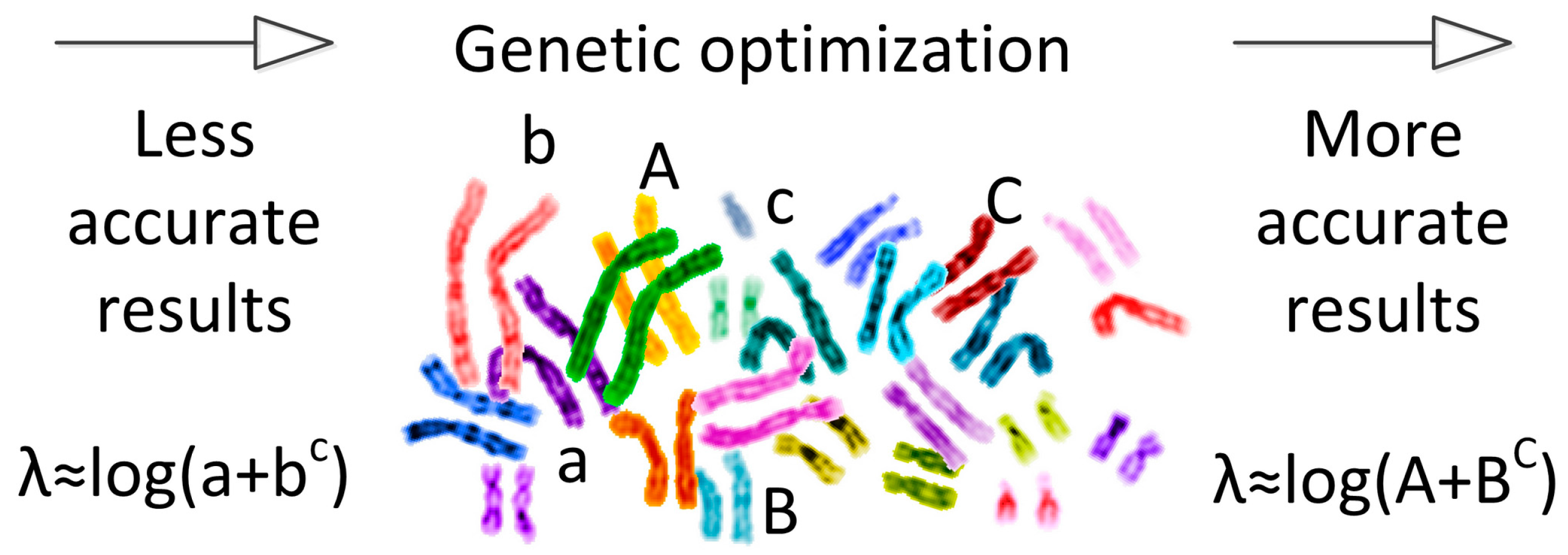
The used optimization approach: Here, the approach with genetic algorithms is implemented to optimize the parameters of the available approximations of the Colebrook equation for the hydraulic friction factor determination in order to improve their accuracy, at the same time retaining the previous complexity and computational burden of approximations. Small letters in the equations throughout the paper correspond to the numerical values before, while capital letters to the numerical values after optimization through genetic algorithms, as is picturesquely presented in Figure 1.
Genetic algorithms are very powerful tools for optimization. Samadianfard [47] uses genetic programming, a sort of genetic algorithm, to develop his own explicit approximations to the Colebrook equation. Furthermore, genetic algorithms can be used together with some other techniques of artificial intelligence, such as neural networks [50,51,52].
Real coded genetic algorithms are used in this paper. The real coded genetic algorithms use the optimization designed cost function that minimizes maximal relative error, δmax, as follow (2):
In (2), δ denotes relative (percentage) error, λ0 denotes the high precision iterative solution of Colebrook’s equation, which is treated as accurate here, λ denotes the hydraulic friction factor solution calculated by each approximation considered and n denotes number of pairs of λ0 and λ used for optimization (in our case, n = 90,000).
The fitness function is evaluated in a large number of 90 thousand points uniformly distributed in domains of the Reynolds number (R) and the relative roughness (ε/D). These domains correspond to those from the Moody diagram [3]; i.e., 2320 < Re < 108, 106 < ε/D < 0.05, where roughness ε usually for PVC and plastic pipes is 0.0015–0.007 mm, copper, lead, brass, aluminum (new) 0.001–0.002 mm and for steel commercial pipe 0.045–0.09 mm. The subjects of genetic optimization are coefficients in approximations, i.e., numeric coefficients in each approximation are changed by genetic algorithms in order to minimize the fitness function (2). In that way, approximations are changed in order to match the accuracy of the iterative solution of Colebrook’s equation as much as possible. Simultaneous optimization of all coefficients in each approximation is attempted, while the range of values of parameters in which optimal solutions are searched is always in the arbitrary neighborhood of the initial values. Here, we chose to present the results obtained with the fitness function (2) in order to reduce the maximal error of each approximation as much as possible (assuming that the reduction of the maximal relative error is of the highest importance for the practical use of approximations). Genetic algorithms’ performance depends on their parameter values, so genetic algorithm parameters were carefully selected by conducting numerous experiments. In the implemented algorithm, a real-coded population of 100 individuals, an elitism of 10 individuals and a scattered crossover function are used. All of the members are subjected to adaptive feasible mutation except for the elite. The individuals are randomly selected by the Roulette method. Optimization with genetic algorithms was carried out in MATLAB R2010a by MathWorks (Natick, MA, USA). The practical domain of the Reynolds number (R) and relative roughness of inner pipe surface (ε/D) are covered by a mesh of n = 90,000 points for this optimization. In these 90 thousand points, the iterative solution of the implicitly-given Colebrook equation, λ0, and the non-iterative solution for every single observed approximation, λ, are calculated. The optimization of every single approximation lasts several hours. All evaluations of error were performed in MATLAB, with further confirmations in MS Excel to maintain full comparability with the study of Brkić [10] (for the use of iterative calculus in MS Excel Ver. 2007, see Brkić [11]; in Brkić and Tanasković [68], MS Excel is also used for other extensive, but non-iterative calculations). The mesh in MS Excel over the practical domain of the Reynolds number (R) and relative roughness of the inner pipe surface (ε/D) consists of n = 740 uniformly-distributed points.
Alternative optimization approaches: The main goal of the optimization in our case is to reduce the maximal error (δmax) of the every single observed approximation. This means that sometimes, the average (mean) relative error in the practical range of the Reynolds number (R) and the relative roughness of inner pipe surface (ε/D) increases compared to the model of the observed approximation with initial, non-optimized values of the parameters. Of course, using genetic algorithm optimization with the function defined to reduce maximal error, this error is reduced more or less efficiently, which at the same time does not mean that average error is necessarily increased or decreased. Although the minimization of average error is not set as a goal by Equation (2), it can be reduced also during the optimization. Instead of the here already shown fitness function Equation (2), it can be redefined to simultaneously reduce average and maximal error Equation (3). In that way, both errors, i.e., maximal relative error and average (mean) relative error, can be reduced simultaneously for sure. This requires more one-off computational efforts compared with the approach in which only one type of error is reduced; in our case, maximal relative error, δmax, while the fitness function is defined by Equation (2). In Equation (3), the first term reduces average (mean) relative error, δavr; the second term reduces maximal error δ; while weights k1 and k2 can be used to signify one of the terms and reduce the influence of other. In that case, a compromise between the reduction of the maximal and average relative error is obtained.
Furthermore, the fitness function can be set to reduce simultaneously the mean square error δMSE and maximal relative error δ, as in Equation (4). As already noted for Equation (3), the ratio between weight coefficients k3 and k4 determines the influence of the mean square error δMSE and the maximal relative error δ in the optimization. According to many different criteria, the values of coefficients in the existing explicit approximation to the Colebrook equation can be used. Using many computational resources, all three errors shown in our paper can be simultaneously reduced Equation (5), but such a procedure seems to be quite elusive.
3. Explicit Approximations of Colebrook’s Equation
Colebrook’s Equation (1) [2] suffers from being implicit in the unknown friction factor (λ). It requires an iterative solution where convergence to the final accuracy of the observed approximation typically requires less than seven iterations. As Brkić [10] proposed, here is used even a few thousand iterations to be sure that a sufficient value of accuracy for the friction factor, λ0, is reached.
As already stated, the implicit Colebrook’s equation cannot be rearranged to derive the friction factor directly in one step, while iterative calculus can cause a problem in the simulation of flow in a pipe system in which it may be necessary to evaluate the friction factor hundreds or thousands of times. This is the main reason for attempting to develop a relationship that is a reasonable and an as accurate as possible approximation for the Colebrook equation, but which is explicit in the friction factor. These approximations are used for the calculation of the friction factor (λ), which is compared with the very accurate solution (λ0) calculated using the iterative procedure.
In this paper, 25 approximations are optimized: Brkić [19,20], Fang et al. [21], Ghanbari et al. [22], Papaevangelou et al. [23], Avci and Karagoz [24], Buzzelli [25], Sonnad and Goudar [26], Romeo et al. [27], Manadilli [28], Chen [29], Serghides [30], Haaland [31], Zigrang and Sylvester [32], Barr [33], Round [34], Shacham (available from [35]), Chen [36], Swamee and Jain [37], Eck [38], Wood [39] and Moody [40]. Ćojbašić and Brkić [42] already optimized the numerical values of the parameters by Romeo et al. [27] and by Serghides [30].
The accuracy of existing approximations of Colebrook’s equation was thoroughly checked by many researchers [10,11,12,13,14,15,16]. Yıldırım [14] conducted a comprehensive analysis of existing correlations for single-phase friction, but he used Techdig 2.0 software to read the date from the Moody diagram, which caused remarkable reading error. One must be always aware that the Moody diagram [3] was constructed using Colebrook’s equation [2] and not opposite. After all, the main conclusion of all papers [10,11,12,13,14,15,16] is that the relative error, δ, is non-uniformly distributed over the domain of the Reynolds number (R) and the relative roughness (ε/D).
The relative error δ is defined in Equations (2)–(4) of this paper, the average (mean) relative error δavr in Equation (3) and the mean square error δMSE in Equation (4). All three types of error are used in further text for the estimation of the accuracy of the examined explicit approximations of the Colebrook equation, but the accent is on the minimization of the maximal relative error, δmax.
Using the shown genetic algorithm optimization technique, the values of existing parameters of the explicit approximations are improved compared to the iterative solution of Colebrook’s equation. This means that the error of approximations decreases while the computational burden stays unchanged. In this section, new parameters are shown, and the reduction of the maximal relative error, δmax, is estimated. The relative errors of the approximations shown in further text of this paper are calculated as δ = [(λ − λ0)/λ0]·100%, where λ is the Darcy friction factor calculated using the observed approximation, while λ0 is the iterative solution of Colebrook’s equation, which can be used as accurate after enough iterations (here, set to the maximal available number of iterations in MS Excel, which is 32,767, as explained in [10]).
Each of the 25 observed approximations is supplied with three diagrams; the first is the distribution of the relative error over the practical domain of applicability in engineering practice; the second is the same as the first, but with the relative error distribution after optimization; and the third is a comparative diagram. For the first two mentioned diagrams, the entire practical domain of the Reynolds number (R) and the relative roughness of the inner pipe surface (ε/D) is covered with a 740 point-mesh (diagrams produced in MS Excel). For the first two figures with approximations, same pace of error is used for non-optimized and for the optimized approximation, to provide a more easy comparison with the exceptions of Approximation (Appr.) 10; Equation (15), Appr. 11; Equation (16) and Appr. 14; Equation (19), where the optimization was extremely successfully performed. The mesh of 740 points is formed in MS Excel using 20 values of the relative roughness (ε/D) (shown in the related figures) and using 37 values of the Reynolds number (R); from 104–105 with a pace of 104, from 105–106 with a pace 105, from 106–107 with a pace of 106 and from 107–108 with a pace of 107.
According to Winning and Coole [16], using the value of mean square error δMSE defined in (4), all approximations can be classified into four groups (the very small error is lower than 10−11; small is between 10−11 and 10−8; medium is between 10−8 and 5 × 10⁻⁶; and large is above 5 × 10⁻⁶). This criterion is also used in further evaluation.
Regarding accuracy, it should be noted that the inner roughness of the pipe, ε, cannot be determined easily [17], so the physical interpretation of the relative roughness of the inner pipe surface (ε/D) is not the subject of this study.
For genetic algorithm optimization, MATLAB 2010a by MathWorks is used. For this purpose, a mesh of 90 thousand points over the entire practical domain of the Reynolds number (R) and the relative roughness of the inner pipe surface (ε/D) is generated. For these 90 thousand pairs of Reynolds number (R) and the relative roughness of inner pipe surface (ε/D), the friction factor (λ0) is very accurately calculated to be used as a pattern during the procedure of optimization. Although genetic optimization allows for virtually all coefficients in each and every formula considered to be optimized in the search for the best result, which can be considered as an important advantage of the presented technique, the selection of the coefficients included in the optimization for each formula was the object of careful consideration. Not only the inclusion of more coefficients significantly widens the search space to be covered, it appears also that some approximations are highly sensitive to the changes of some coefficients. Therefore, subsets of coefficients to be optimized within each formula were selected on the basis of multiple trials, approaches considered by other authors and our own vast experience. The number of digits in each optimized coefficient was also limited as a tradeoff of the desired punctuality of approximation and the practical usability of the formula.
The efficiency of computing in the computer environment stays unchanged between non-optimized and related optimized approximations, since the model of the approximation stays unchanged; i.e., the number of logarithmic and power expressions stays unchanged [9,18]. Only the change of integer power to non-integer power in some approximation can increase the computational burden, but even then not significantly.
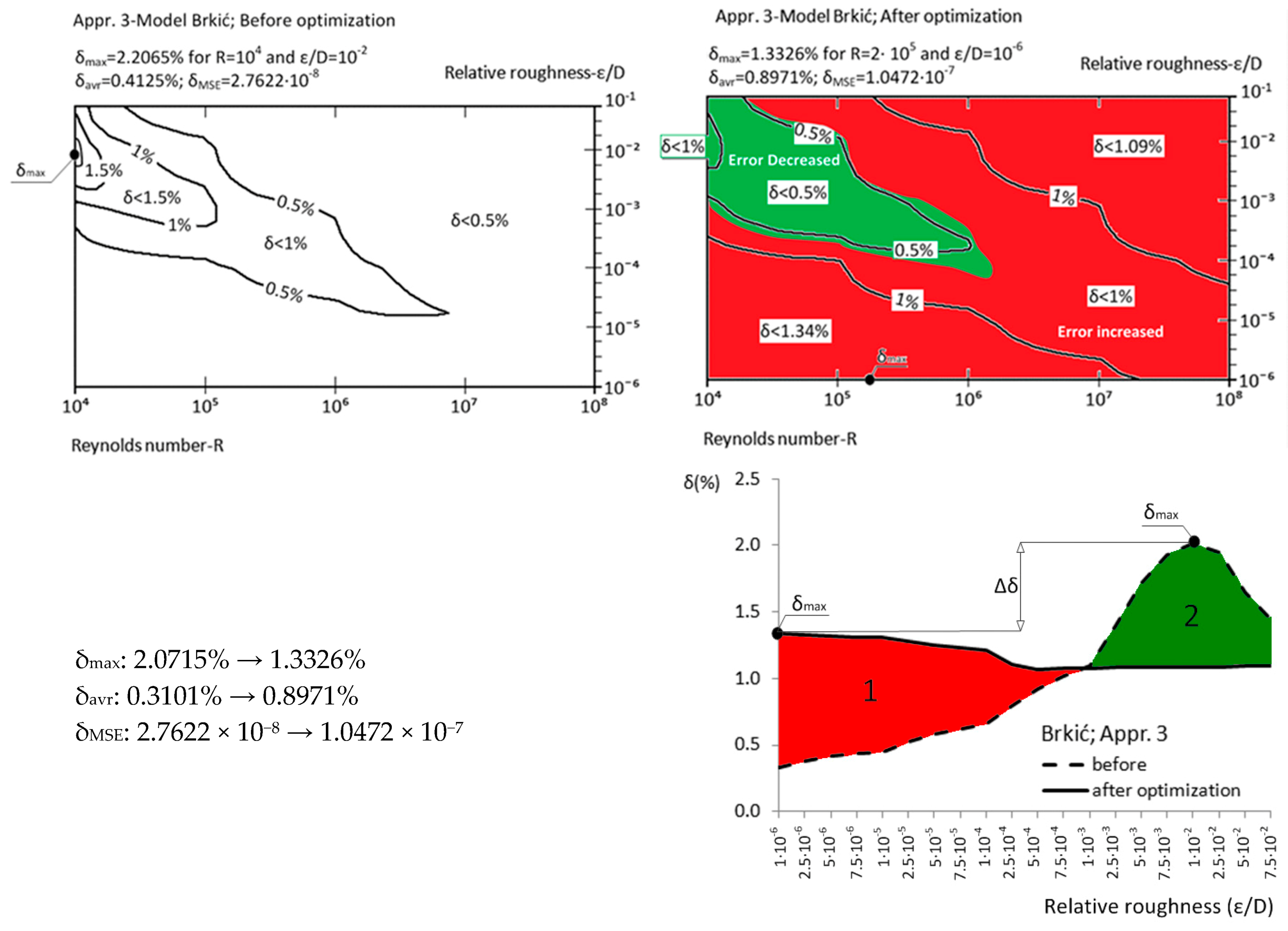
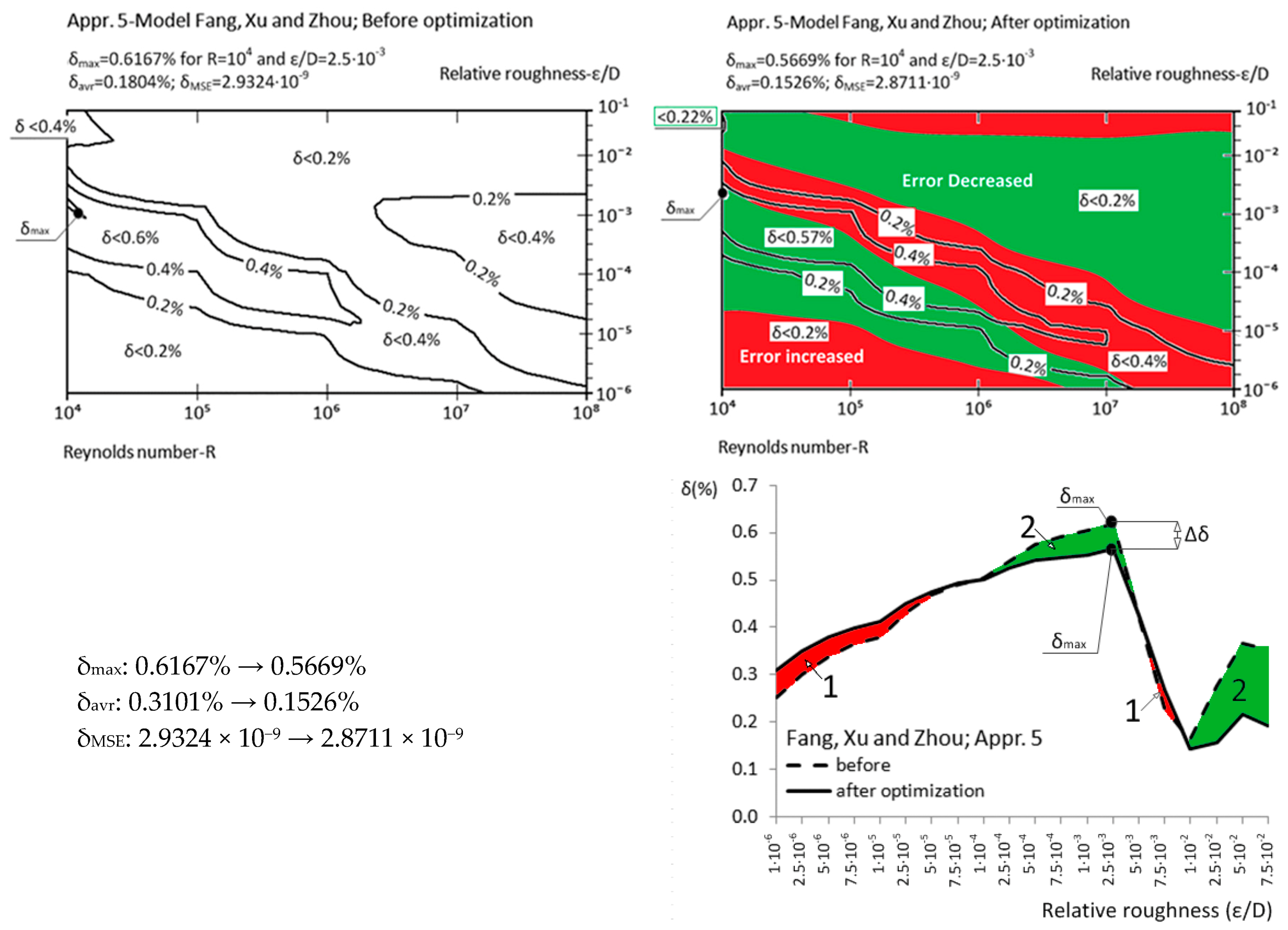
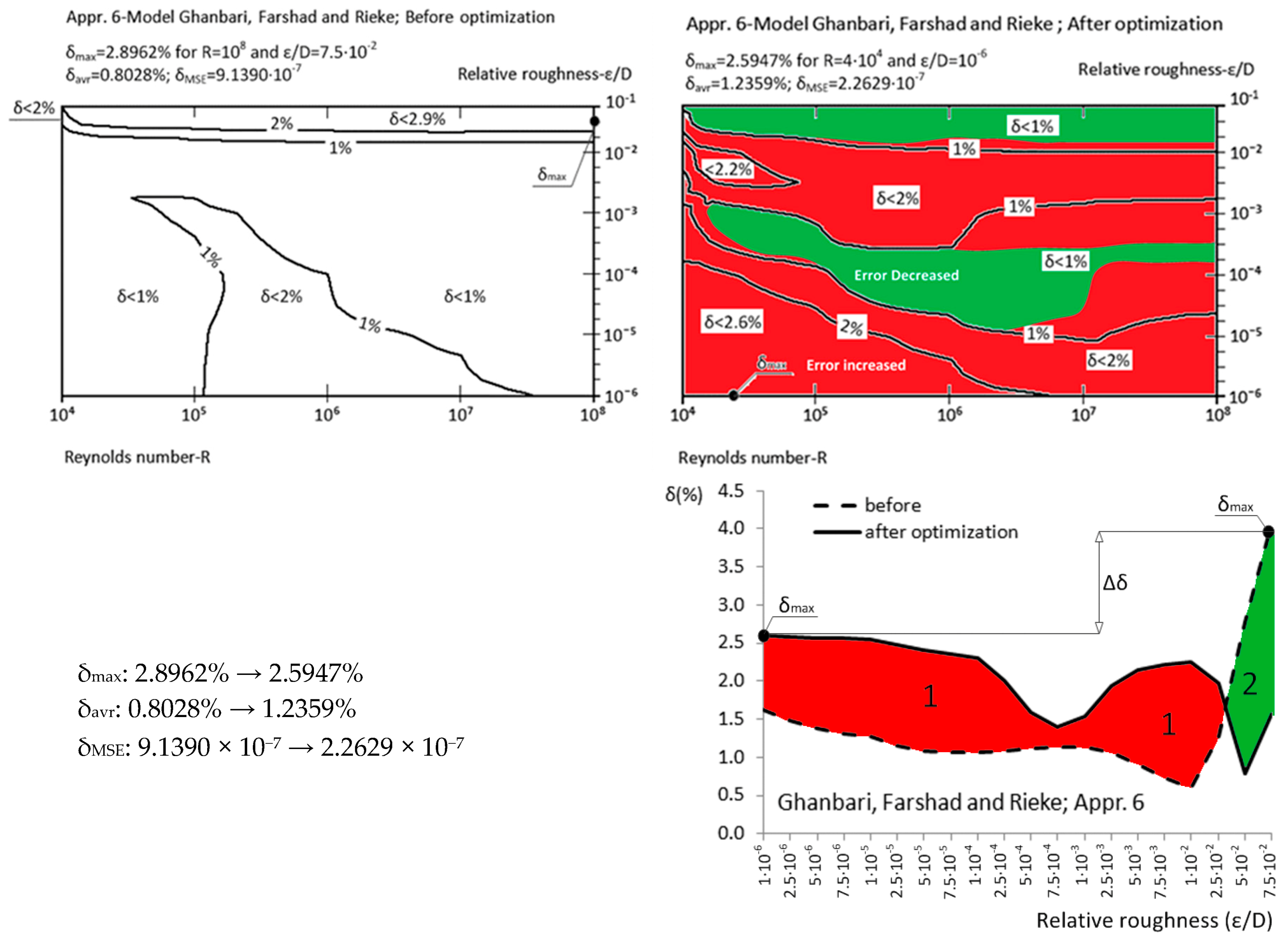
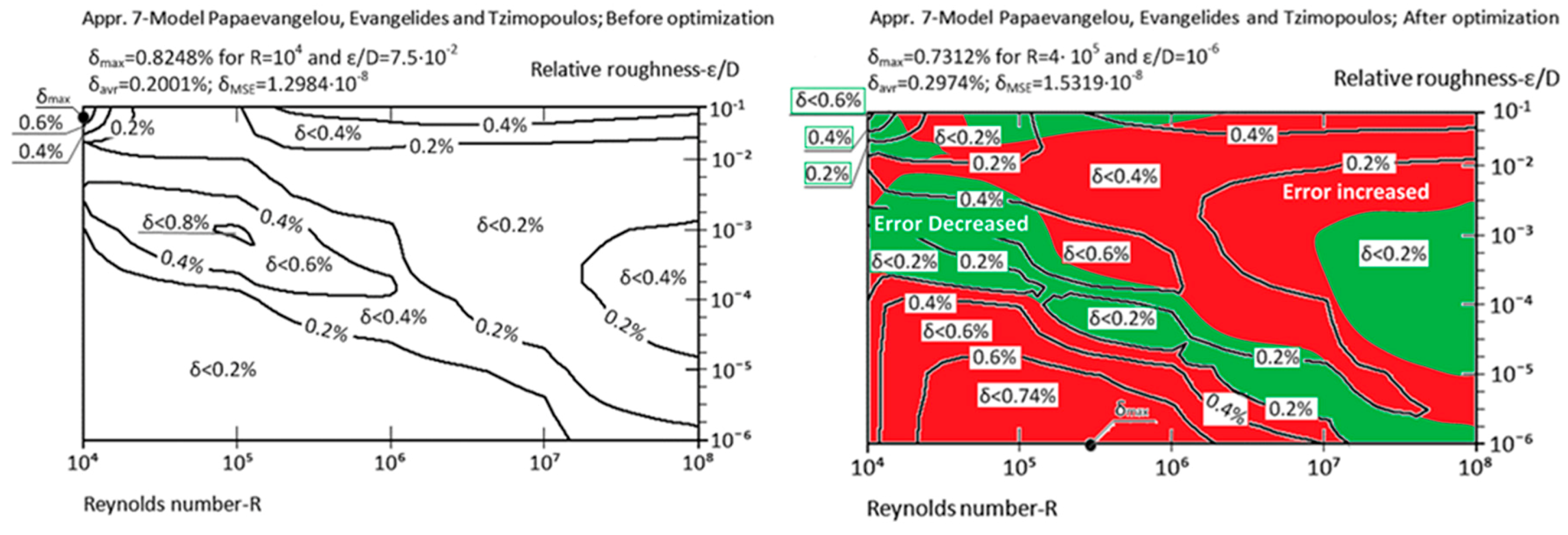
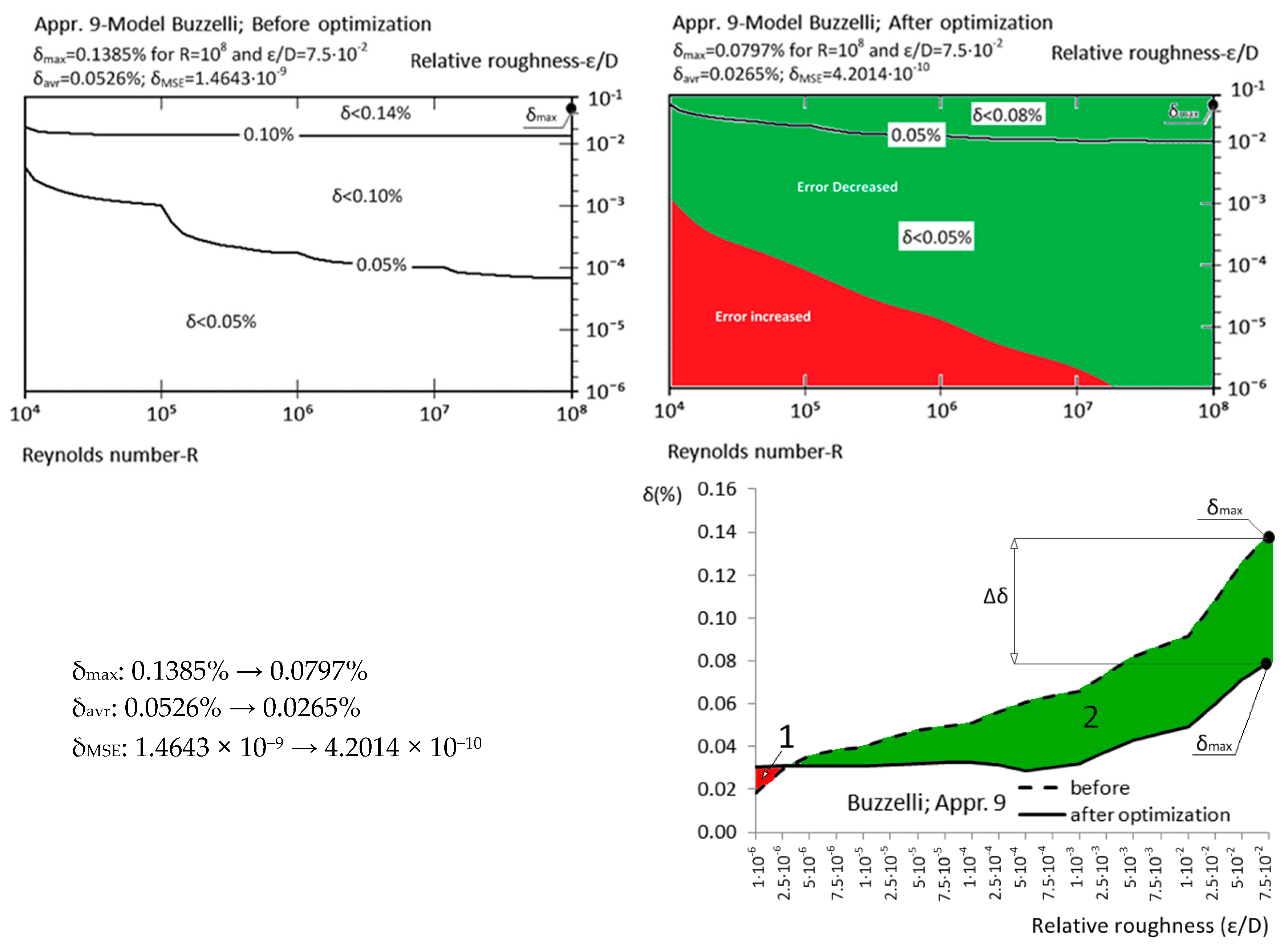
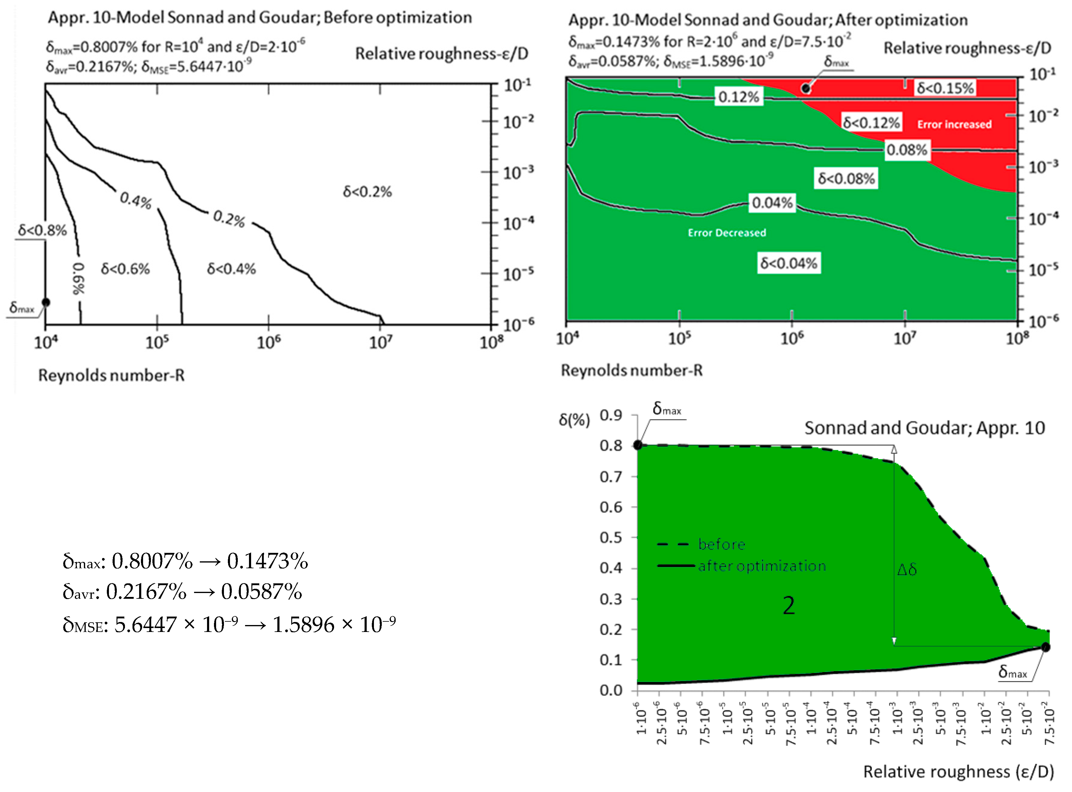
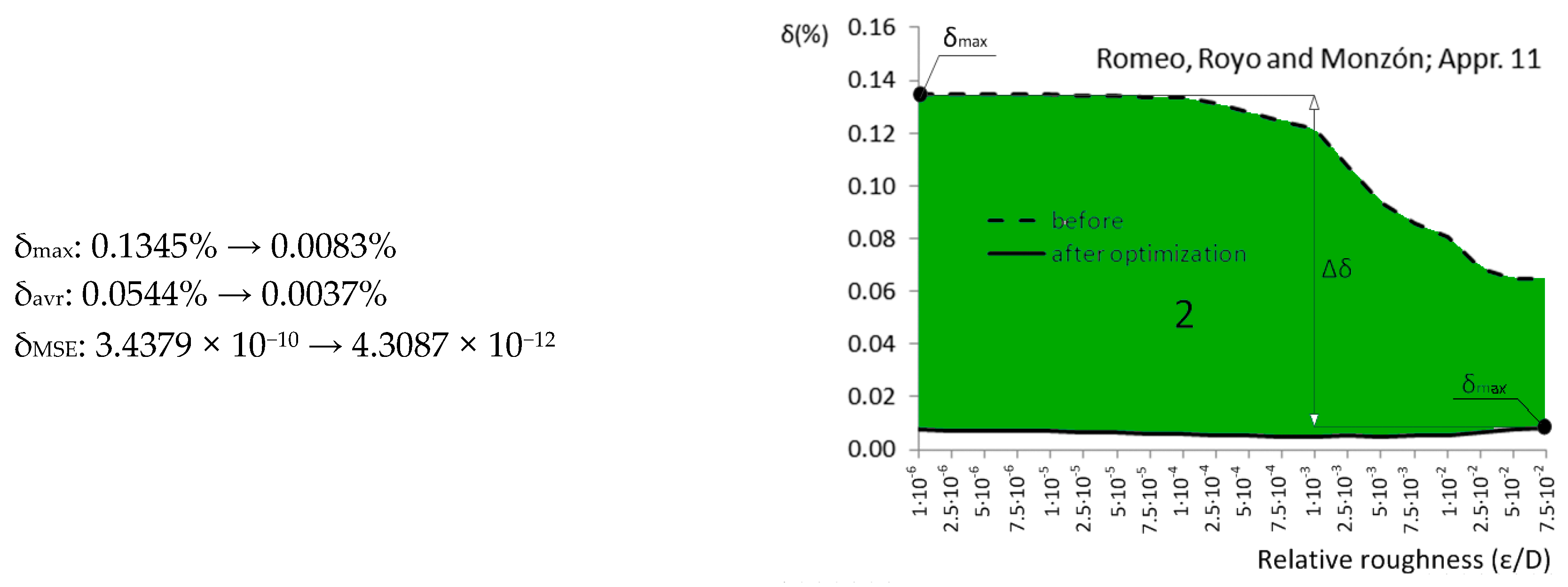
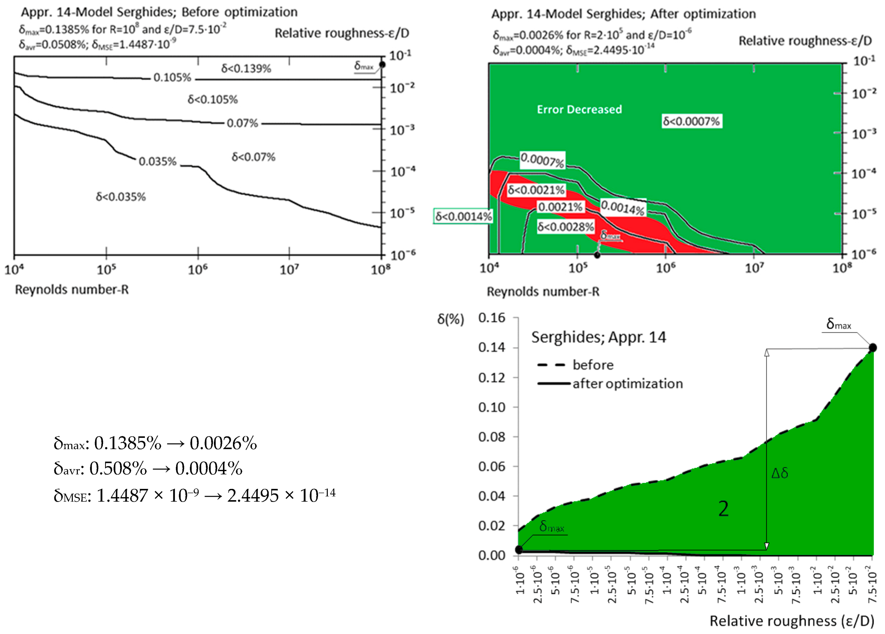
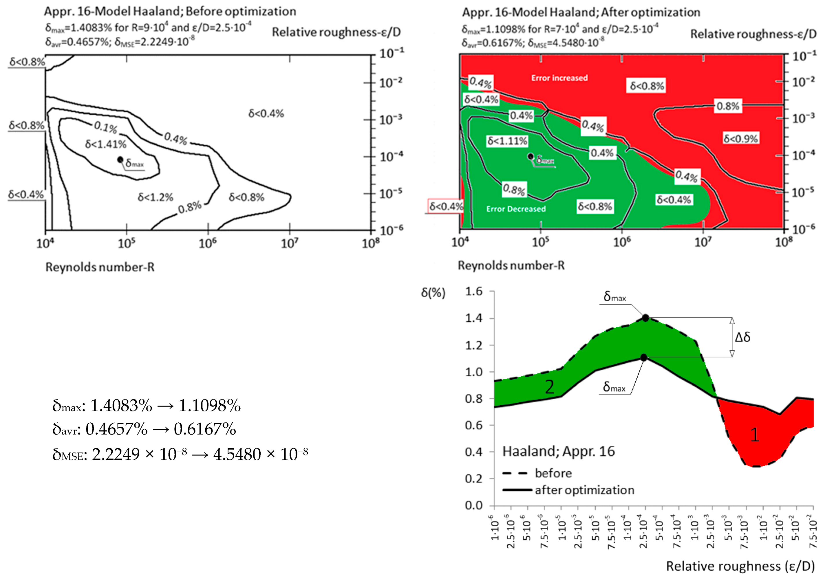
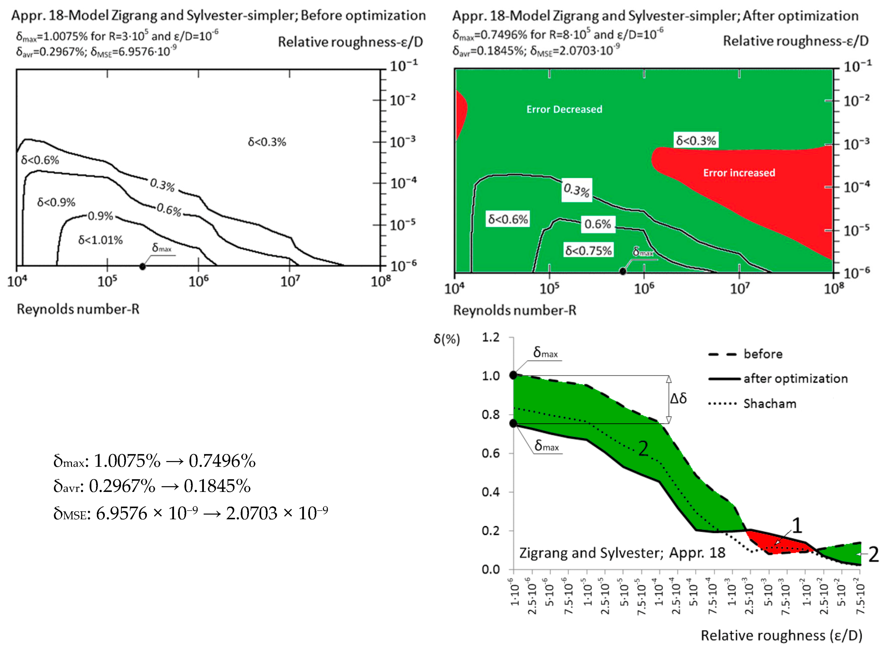
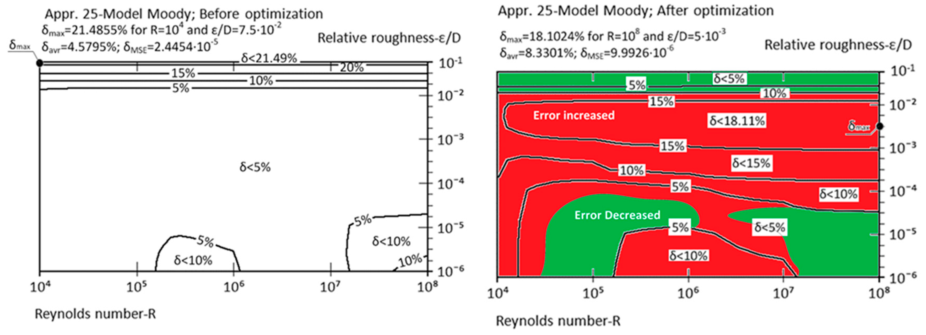
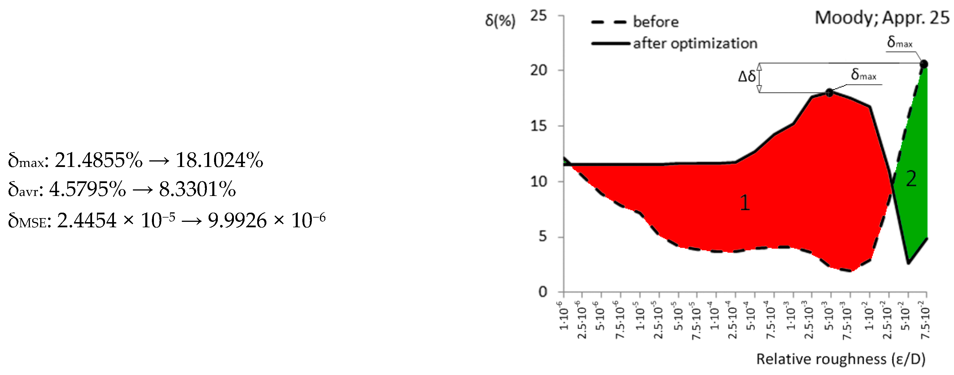
In the following Figure 2, Figure 3, Figure 4, Figure 5, Figure 6, Figure 7, Figure 8, Figure 9, Figure 10, Figure 11, Figure 12, Figure 13, Figure 14, Figure 15, Figure 16, Figure 17, Figure 18, Figure 19, Figure 20, Figure 21, Figure 22, Figure 23, Figure 24, Figure 25 and Figure 26, symbols and zones with green and red color represent: the Δδ-decreased level of maximal relative error δmax; (1) zone of increased relative error δ (red); (2) zone of decreased relative error δ (green).
Brkić approximation (Appr. 1): Relevant parameters and errors related to the approximation by Brkić [19] after and before optimization (6) (Appr. 1) are given in Figure 2.
Brkić approximation (Appr. 2): Relevant parameters and errors related to the approximation by Brkić [19] after and before optimization (7) (Appr. 2) are given in Figure 3.
Brkić approximation (Appr. 3): Relevant parameters and errors related to the approximation by Brkić [20] after and before optimization (8) (Appr. 3) are given in Figure 4.
Brkić approximation (Appr. 4): Relevant parameters and errors related to the approximation by Brkić [20] after and before optimization (9) (Appr. 4) are given in Figure 5.
Fang et al. approximation (Appr. 5): Relevant parameters and errors related to the approximation by Fang et al. [21] after and before optimization (10) (Appr. 5) are given in Figure 6.
Ghanbari, Farshad and Rieke approximation (Appr. 6): Relevant parameters and errors related to the approximation by Ghanbari et al. [22] after and before optimization (11) (Appr. 6) are given in Figure 7.
Papaevangelou, Evangelides and Tzimopoulos approximation (Appr. 7): Relevant parameters and errors related to the approximation by Papaevangelou et al. [23] after and before optimization (12) (Appr. 7) are given in Figure 8.
Avci and Karagoz approximation (Appr. 8): Relevant parameters and errors related to the approximation by Avci and Karagoz [24] after and before optimization (13) (Appr. 8) are given in Figure 9.
Buzzelli approximation (Appr. 9): Relevant parameters and errors related to the approximation by Buzzelli [25] after and before optimization (14) (Appr. 9) are given in Figure 10.
Sonnad and Goudar approximation (Appr. 10): Relevant parameters and errors related to the approximation by Sonnad and Goudar [26] after and before optimization (15) (Appr. 10) are given in Figure 11. Vatankhah and Kouchakzadeh [43,44] by changing parameter ɑ11 to A11-0.31 slightly change the model of Sonnad and Goudar [26]. They used line fitting tool for optimization. We failed with further optimization using genetic algorithms.
Romeo, Royo and Monzón approximation (Appr. 11): Relevant parameters and errors related to the approximation by Romeo et al. [27] after and before optimization (16) (Appr. 11) are given in Figure 12; already shown in the form of the preliminary note in Ćojbašić and Brkić [42].
Manadilli approximation (Appr. 12): Relevant parameters and errors related to the approximation by Manadilli [28] after and before optimization (17) (Appr. 12) are given in Figure 13.
Chen approximation (Appr. 13): Relevant parameters and errors related to the approximation by Chen [29] after and before optimization (18) (Appr. 13) are given in Figure 14.
Serghides approximation (Appr. 14): Relevant parameters and errors related to the approximation by Serghides [30] after and before optimization (19) (Appr. 14) are given in Figure 15. This optimization is already shown in the form of the preliminary note in Ćojbašić and Brkić [42].
Serghides approximation (simpler) (Appr. 15): Relevant parameters and errors related to the approximation by Serghides (simpler) [30] after and before optimization (20) (Appr. 15) are given in Figure 16.
Haaland approximation (Appr. 16): Relevant parameters and errors related to the approximation by Haaland [31] after and before optimization (21) (Appr. 16) are given in Figure 17.
Zigrang and Sylvester approximation (Appr. 17): Relevant parameters and errors related to the approximation by Zigrang and Sylvester [32] after and before optimization (22) (Appr. 17) are given in Figure 18.
Zigrang and Sylvester approximation (simpler) (Appr. 18): Relevant parameters and errors related to the approximation by Zigrang and Sylvester (simpler) [32] after and before optimization (23) (Appr. 18) are given in Figure 19.
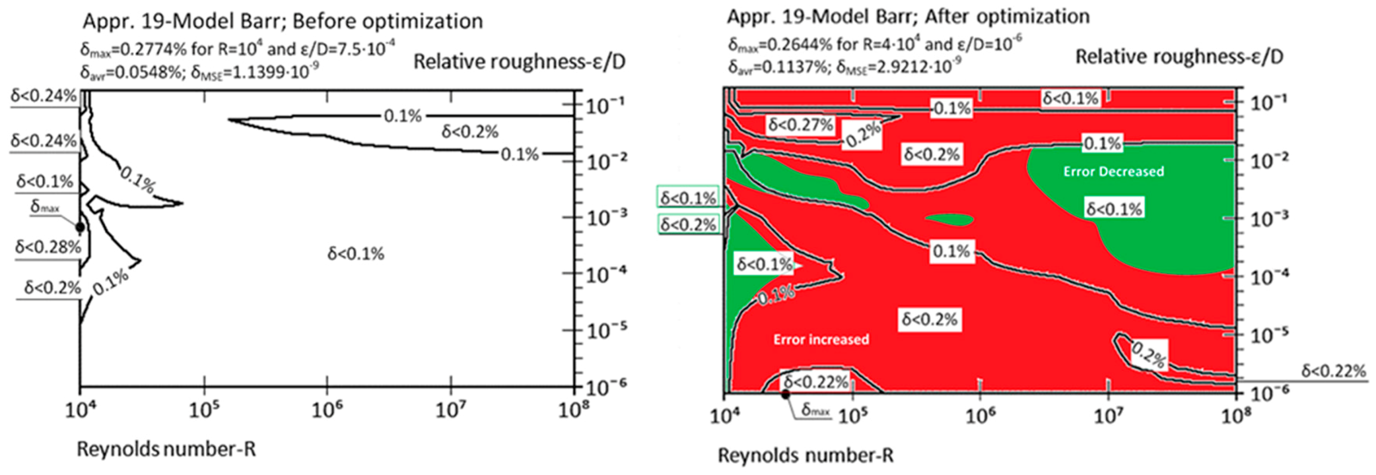
Barr approximation (Appr. 19): Relevant parameters and errors related to the approximation by Barr [33] after and before optimization (24) (Appr. 19) are given in Figure 20.
Round approximation (Appr. 20): Relevant parameters and errors related to the approximation by Round [34] after and before optimization (25) (Appr. 20) are given in Figure 21.
Chen approximation (Appr. 21) Relevant parameters and errors related to the approximation by Chen [36] after and before optimization (26) (Appr. 21) are given in Figure 22.
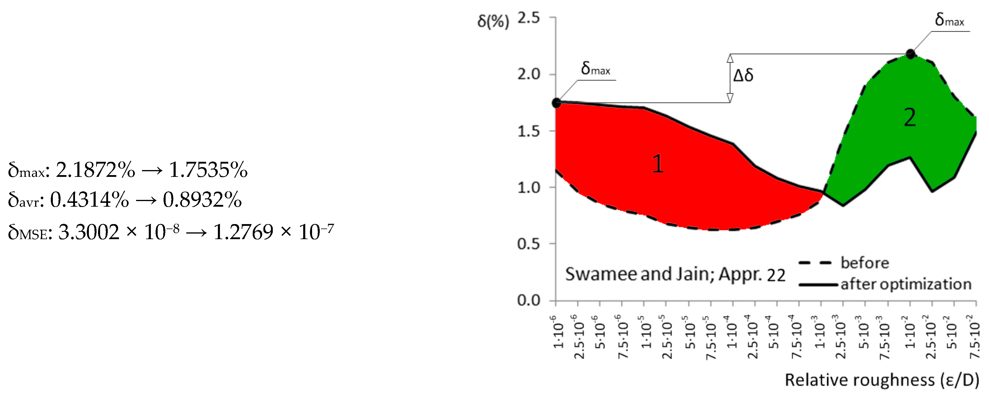
Swamee and Jain approximation (Appr. 22): Relevant parameters and errors related to the approximation by Swamee and Jain [37] after and before optimization (27) (Appr. 22) are given in Figure 23.
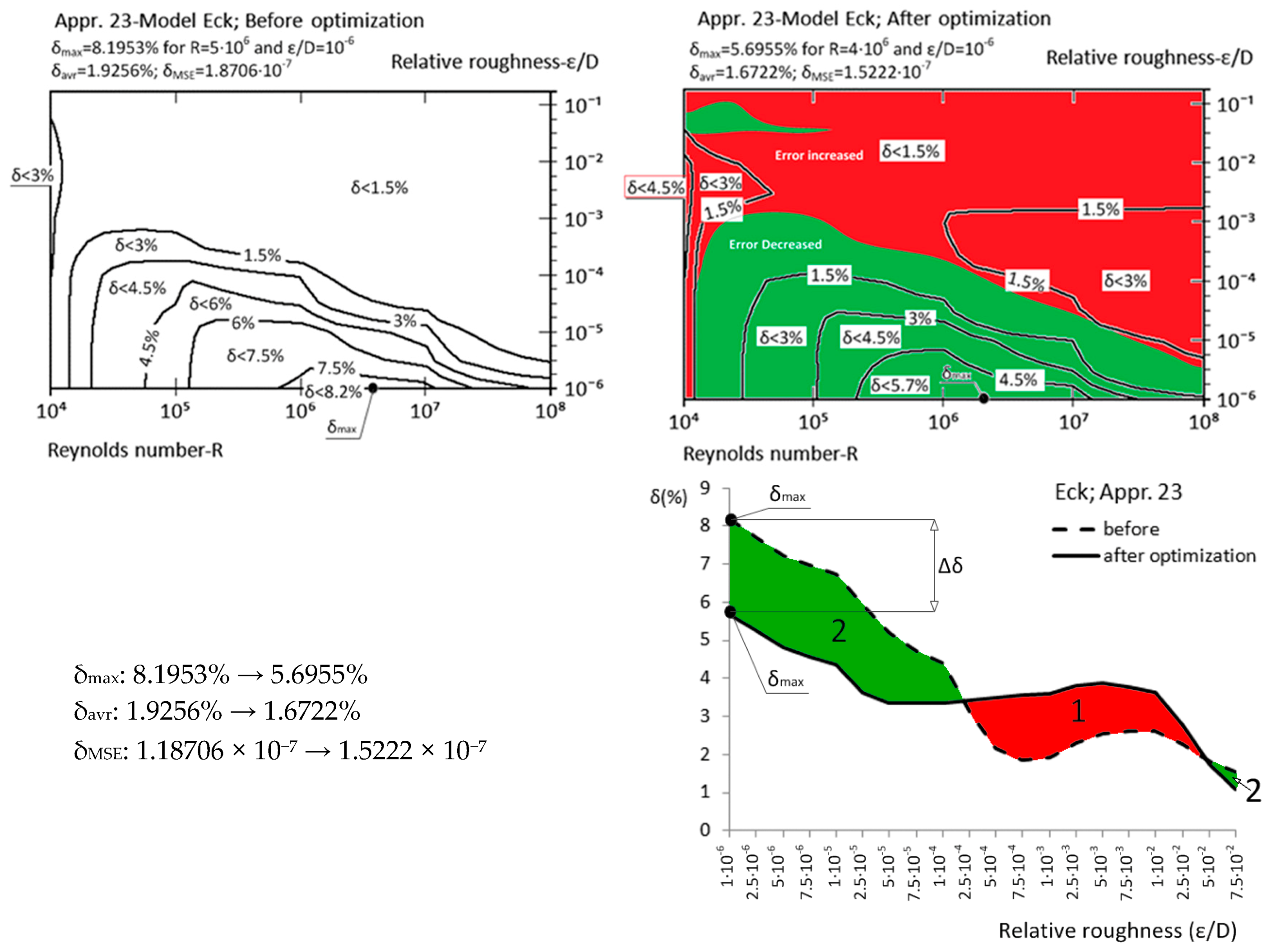
Eck approximation (Appr. 23): Relevant parameters and errors related to the approximation by Eck [38] after and before optimization (28) (Appr. 23) are given in Figure 24.
4. Conclusions
Today, Colebrook’s equation is mostly accepted as an informal standard for the modeling of turbulent flow in hydraulically smooth and rough pipes, including the transient zone in between. Of course, approximations carry certain error compared with the iterative solution where the highest level of accuracy can be reached after enough iterations. The explicit approximations give a relatively good prediction of the friction factor (λ) and can reproduce accurately Colebrook’s equation and its Moody’s plot. Usually, more complex models of approximations are more accurate and vice versa. Using genetic algorithms in order to increase the accuracy of available approximations of the Colebrook equation for flow friction, the numerical values of empirical parameters in 25 existing models of approximations are changed while the computational burden remains the same. Using the value of decreased maximal relative error, Δδ, and the change of relative error over the entire domain of the Reynolds number (R) and the relative roughness of inner pipe surface (ε/D), the success of genetic optimization is summarized in Table 1.
Since the main idea of this study was to use metaheuristic optimization to improve the accuracy of a wider set of Colebrook’s turbulent flow friction approximations, as opposed to other approaches used by other authors and ourselves, Genetic Algorithms were selected as being referential among global optimization techniques. Additional accuracy for the certain approximations can be possibly reached through rearrangement of their structure (such as was done for Appr. 10 [26,43]), using the MS Excel fitting tool [49], etc. Furthermore, some further use of genetic algorithms can be encouraged. Future research directions could include also the application of other metaheuristic optimization techniques for the same task, such as particle swarm optimization (PSO), ant colony optimization (ACO), simulated annealing (SA) and others [69,70,71]. Further accuracy improvements might be possible, but the highest accuracy approximations have already been optimized to extremely high precision levels regarding practical application.
During this study, it is found that the criterion from Winning and Coole [16] about the accuracy of approximations using the value of mean square error should be modified as: very small error is lower than 10−10; small is between 10−10 and 10−8; medium is between 10−8 and 5 × 10⁻⁷; and large is above 5 × 10⁻⁷. The criterion of accuracy using the value of maximal relative error δmax should be set as: very small error is lower than 0.2%; small is between 0.2% and 1%; medium is between 1% and 3%; and large is above 3% (extremely large above 5%). Furthermore, it is found that the error distribution, set as a criterion in Winning and Coole [16], does not depend only on the model of approximation, but changes equally with the change of the values of the parameters.
Aside from the Colebrook equation, the presented methodology can be used to fit the raw and updated measured data, all similar empirical equations that cover the same region of turbulent flow [54,55]. The friction factor curves derived from the Colebrook equation are said to be monotonic, i.e., the friction factor (λ) decreases continuously with increasing Reynolds number (R). For some tests carried out on pipes that were artificially roughened with grains of sand, the curves were inflectional in nature, i.e., the friction factor (λ) decreases to a minimum value with increasing Reynolds number (R) and then rises again to reach a constant value for complete turbulence [53,54]. The proposed optimization procedure can be used also to fit such data.
Supplementary Materials
Excel and MATLAB codes of the approximations presented in this paper are available online at www.mdpi.com/2311-5521/2/2/15/s1.
Acknowledgments
The work of Žarko Ćojbašić has been supported by the Ministry of Education, Science and Technological Development of the Republic of Serbia under Grants TR35016 and TR35005.
Author Contributions
Dejan Brkić has scientific interest in hydraulics, and he prepared data related to flow friction, checked the accuracy of the final results, drew diagrams and wrote the manuscript. Žarko Ćojbašić has scientific interest in artificial intelligence, and he performed optimization using genetic algorithms. Both authors contributed equally to this study (the authors are listed alphabetically according to their surnames).
Conflicts of Interest
The views expressed are those of the authors and may not in any circumstances be regarded as stating an official position of the European Commission or the University of Niš.
References
- Colebrook, C.F.; White, C.M. Experiments with fluid friction in roughened pipes. Proc. R. Soc. Ser. A Math. Phys. Sci. 1937, 161, 367–381. [Google Scholar] [CrossRef]
- Colebrook, C.F. Turbulent flow in pipes with particular reference to the transition region between the smooth and rough pipe laws. J. Inst. Civ. Eng. (Lond.) 1939, 11, 133–156. [Google Scholar] [CrossRef]
- Moody, L.F. Friction factors for pipe flow. Trans. ASME 1944, 66, 671–684. [Google Scholar]
- LaViolette, M. On the history, science, and technology included in the Moody diagram. J. Fluids Eng. ASME 2017, 139, 030801. [Google Scholar] [CrossRef]
- Mikata, Y.; Walczak, W.S. Exact analytical solutions of the Colebrook-White equation. J. Hydraul. Eng. ASCE 2016, 142. [Google Scholar] [CrossRef]
- Brkić, D. W solutions of the CW equation for flow friction. Appl. Math. Lett. 2011, 24, 1379–1383. [Google Scholar] [CrossRef]
- Biberg, D. Fast and accurate approximations for the Colebrook equation. J. Fluids Eng. ASME 2017, 139, 031401. [Google Scholar] [CrossRef]
- Keady, G. Colebrook-White formula for pipe flow. J. Hydraul. Eng. ASCE 1998, 124, 96–97. [Google Scholar] [CrossRef]
- Clamond, D. Efficient resolution of the Colebrook equation. Ind. Eng. Chem. Res. 2009, 48, 3665–3671. [Google Scholar] [CrossRef]
- Brkić, D. Review of explicit approximations to the Colebrook relation for flow friction. J. Petrol. Sci. Eng. 2011, 77, 34–48. [Google Scholar] [CrossRef]
- Brkić, D. Determining friction factors in turbulent pipe flow. Chem. Eng. (N. Y.) 2012, 119, 34–39. [Google Scholar]
- Gregory, G.A.; Fogarasi, M. Alternate to standard friction factor equation. Oil Gas J. 1985, 83, 125–127. [Google Scholar]
- Zigrang, D.J.; Sylvester, N.D. A review of explicit friction factor equations. J. Energy Resour. Technol. ASME 1985, 107, 280–283. [Google Scholar] [CrossRef]
- Yıldırım, G. Computer-based analysis of explicit approximations to the implicit Colebrook-White equation in turbulent flow friction factor calculation. Adv. Eng. Softw. 2009, 40, 1183–1190. [Google Scholar] [CrossRef]
- Genić, S.; Aranđelović, I.; Kolendić, P.; Jarić, M.; Budimir, N.; Genić, V. A review of explicit approximations of Colebrook’s equation. FME Trans. 2011, 39, 67–71. [Google Scholar]
- Winning, H.K.; Coole, T. Explicit friction factor accuracy and computational efficiency for turbulent flow in pipes. Flow Turbul. Combust. 2013, 90, 1–27. [Google Scholar] [CrossRef]
- Lira, I. On the uncertainties stemming from use of the Colebrook-White equation. Ind. Eng. Chem. Res. 2013, 52, 7550–7555. [Google Scholar] [CrossRef]
- Giustolisi, O.; Berardi, L.; Walski, T.M. Some explicit formulations of Colebrook–White friction factor considering accuracy vs. computational speed. J. Hydroinformatics 2011, 13, 401–418. [Google Scholar] [CrossRef]
- Brkić, D. An explicit approximation of the Colebrook equation for fluid flow friction factor. Petrol. Sci. Technol. 2011, 29, 1596–1602. [Google Scholar] [CrossRef]
- Brkić, D. New explicit correlations for turbulent flow friction factor. Nucl. Eng. Des. 2011, 241, 4055–4059. [Google Scholar] [CrossRef]
- Fang, X.; Xu, Y.; Zhou, Z. New correlations of single-phase friction factor for turbulent pipe flow and evaluation of existing single-phase friction factor correlations. Nucl. Eng. Des. 2011, 241, 897–902. [Google Scholar] [CrossRef]
- Ghanbari, A.; Farshad, F.F.; Rieke, H.H. Newly developed friction factor correlation for pipe flow and flow assurance. J. Chem. Eng. Mater. Sci. 2011, 2, 83–86. [Google Scholar]
- Papaevangelou, G.; Evangelides, C.; Tzimopoulos, C. A new explicit relation for the friction factor coefficient in the Darcy–Weisbach equation. In Proceedings of the Protection and Restoration of the Environment, Corfu, Greece, 5–9 July 2010; pp. 166–172. [Google Scholar]
- Avci, A.; Karagoz, I. A novel explicit equation for friction factor in smooth and rough pipes. J. Fluids Eng. ASME 2009, 131, 061203. [Google Scholar] [CrossRef]
- Buzzelli, D. Calculating friction in one step. Mach. Des. 2008, 80, 54–55. [Google Scholar]
- Sonnad, J.R.; Goudar, C.T. Turbulent flow friction factor calculation using a mathematically exact alternative to the Colebrook–White equation. J. Hydraul. Eng. ASCE 2006, 132, 863–867. [Google Scholar] [CrossRef]
- Romeo, E.; Royo, C.; Monzón, A. Improved explicit equations for estimation of the friction factor in rough and smooth pipes. Chem. Eng. J. 2002, 86, 369–374. [Google Scholar] [CrossRef]
- Manadilli, G. Replace implicit equations with signomial functions. Chem. Eng. (N. Y.) 1997, 104, 129–130. [Google Scholar]
- Chen, J.J.J. A simple explicit formula for the estimation of pipe friction factor. Proc. Inst. Civ. Eng. 1984, 77, 49–55. [Google Scholar] [CrossRef]
- Serghides, T.K. Estimate friction factor accurately. Chem. Eng. (N. Y.) 1984, 91, 63–64. [Google Scholar]
- Haaland, S.E. Simple and explicit formulas for the friction factor in turbulent pipe flow. J. Fluids Eng. ASME 1983, 105, 89–90. [Google Scholar] [CrossRef]
- Zigrang, D.J.; Sylvester, N.D. Explicit approximations to the solution of Colebrook’s friction factor equation. AIChE J. 1982, 28, 514–515. [Google Scholar] [CrossRef]
- Barr, D.I.H. Solutions of the Colebrook-White function for resistance to uniform turbulent flow. Proc. Inst. Civ. Eng. 1981, 71, 529–535. [Google Scholar]
- Round, G.F. An explicit approximation for the friction factor-Reynolds number relation for rough and smooth pipes. Can. J. Chem. Eng. 1980, 58, 122–123. [Google Scholar] [CrossRef]
- Schorle, B.J.; Churchill, S.W.; Shacham, M. Comments on: “An explicit equation for friction factor in pipe”. Ind. Eng. Chem. Fundam. 1980, 19, 228–230. [Google Scholar] [CrossRef]
- Chen, N.H. An explicit equation for friction factor in pipes. Ind. Eng. Chem. Fundam. 1979, 18, 296–297. [Google Scholar] [CrossRef]
- Swamee, D.K.; Jain, A.K. Explicit equations for pipe flow problems. J. Hydraul. Div. ASCE 1976, 102, 657–664. [Google Scholar]
- Eck, B. Technische Stromungslehre; Springer: New York, NY, USA, 1973. [Google Scholar]
- Wood, D.J. An explicit friction factor relationship. Civ. Eng. 1966, 36, 60–61. [Google Scholar]
- Moody, L.F. An approximate formula for pipe friction factors. Trans. ASME 1947, 69, 1005–1006. [Google Scholar]
- Brkić, D. A note on explicit approximations to Colebrook’s friction factor in rough pipes under highly turbulent cases. Int. J. Heat Mass Tran. 2016, 93, 513–515. [Google Scholar] [CrossRef]
- Ćojbašić, Ž.; Brkić, D. Very accurate explicit approximations for calculation of the Colebrook friction factor. Int. J. Mech. Sci. 2013, 67, 10–13. [Google Scholar] [CrossRef]
- Vatankhah, A.R.; Kouchakzadeh, S. Discussion of Turbulent flow friction factor calculation using a mathematically exact alternative to the Colebrook-White equation. J. Hydraul. Eng. ASCE 2008, 134, 1187. [Google Scholar] [CrossRef]
- Vatankhah, A.R.; Kouchakzadeh, S. Discussion: Exact equations for pipe-flow problems. J. Hydraul. Res. IAHR 2009, 47, 537–538. [Google Scholar] [CrossRef]
- Goldberg, D.E. Genetic Algorithms in Search, Optimization and Machine Learning; Addison-Wesley Inc.: Reston, VA, USA, 1989. [Google Scholar]
- Fleming, P.J.; Purshouse, R.C. Evolutionary algorithms in control systems engineering: A survey. Control Eng. Pract. 2002, 10, 1223–1241. [Google Scholar] [CrossRef]
- Samadianfard, S. Gene expression programming analysis of implicit Colebrook-White equation in turbulent flow friction factor calculation. J. Petrol. Sci. Eng. 2012, 92–93, 48–55. [Google Scholar] [CrossRef]
- Brkić, D. Discussion of “Gene expression programming analysis of implicit Colebrook–White equation in turbulent flow friction factor calculation”. J. Petrol. Sci. Eng. 2014, 124, 399–401. [Google Scholar] [CrossRef]
- Vatankhah, A.R. Comment on “Gene expression programming analysis of implicit Colebrook–White equation in turbulent flow friction factor calculation”. J. Petrol. Sci. Eng. 2014, 124, 402–405. [Google Scholar] [CrossRef]
- Brkić, D.; Ćojbašić, Ž. Intelligent flow friction estimation. Comput. Intell. Neurosci. 2016, 2016, 5242596. [Google Scholar] [CrossRef] [PubMed]
- Ćojbašić, Ž.; Nikolić, V.; Petrović, E.; Pavlović, V.; Tomić, M.; Pavlović, I.; Ćirić, I. A real time neural network based finite element analysis of shell structure. Facta Univ. Mech. Eng. 2014, 12, 149–155. [Google Scholar]
- Dučić, N.; Ćojbašić, Ž.; Radiša, R.; Slavković, R.; Milićević, M. CAD/CAM design and genetic optimization of feeders for sand casting process. Facta Univ. Mech. Eng. 2016, 14, 147–158. [Google Scholar]
- Brkić, D. Efficiency of Distribution and Use of Natural Gas in Households (Ефикасност дистрибуције и коришћења природног гаса у домаћинствима, In Serbian). Ph.D. Thesis, University of Belgrade, Belgrade, Serbia, 2010. [Google Scholar]
- Allen, J.J.; Shockling, M.A.; Kunkel, G.J.; Smits, A.J. Turbulent flow in smooth and rough pipes. Proc. R. Soc. Ser. A Math. Phys. Sci. 2007, 365, 699–714. [Google Scholar] [CrossRef] [PubMed]
- Brkić, D. A gas distribution network hydraulic problem from practice. Petrol. Sci. Technol. 2011, 29, 366–377. [Google Scholar] [CrossRef]
- Brkić, D. Can pipes be actually really that smooth? Int. J. Refrig. 2012, 35, 209–215. [Google Scholar] [CrossRef]
- Brkić, D. Discussion of “Jacobian matrix for solving water distribution system equations with the Darcy-Weisbach head-loss model”. J. Hydraul. Eng. ASCE 2012, 138, 1000–1002. [Google Scholar] [CrossRef]
- Brkić, D. Discussion of “Water distribution system analysis: Newton-Raphson method revisited”. J. Hydraul. Eng. ASCE 2012, 138, 822–824. [Google Scholar] [CrossRef]
- Brkić, D. Discussion of “Method to cope with zero flows in newton solvers for water distribution systems”. J. Hydraul. Eng. ASCE 2014, 140, 07014003. [Google Scholar] [CrossRef]
- Sonnad, J.R.; Goudar, C.T. Constraints for using Lambert W function-based explicit Colebrook–White equation. J. Hydraul. Eng. ASCE 2004, 130, 929–931. [Google Scholar] [CrossRef]
- Brkić, D. Comparison of the Lambert W-function based solutions to the Colebrook equation. Eng. Comput. 2012, 29, 617–630. [Google Scholar] [CrossRef]
- Rollmann, P.; Spindler, K. Explicit representation of the implicit Colebrook–White equation. Case Stud. Therm. Eng. 2015, 5, 41–47. [Google Scholar] [CrossRef]
- Brkić, D. Spreadsheet-based pipe networks analysis for teaching and learning purpose. Spreadsheets Educ. (eJSiE) 2016, 9. Available online: http://epublications.bond.edu.au/ejsie/vol9/iss2/4/ (accessed on 03 April 2017).
- Brkić, D. Iterative methods for looped network pipeline calculation. Water Resour. Manag. 2011, 25, 2951–2987. [Google Scholar] [CrossRef]
- Simpson, A.; Elhay, S. Jacobian matrix for solving water distribution system equations with the Darcy-Weisbach head-loss model. J. Hydraul. Eng. ASCE 2011, 137, 696–700. [Google Scholar] [CrossRef]
- Spiliotis, M.; Tsakiris, G. Water distribution system analysis: Newton-Raphson method revisited. J. Hydraul. Eng. ASCE 2011, 137, 852–855. [Google Scholar] [CrossRef]
- Brkić, D. An improvement of Hardy Cross method applied on looped spatial natural gas distribution networks. Appl. Energy 2009, 86, 1290–1300. [Google Scholar] [CrossRef]
- Brkić, D.; Tanasković, T. Systematic approach to natural gas usage for domestic heating in urban areas. Energy 2008, 33, 1738–1753. [Google Scholar] [CrossRef]
- Ćojbašić, Ž.; Petković, D.; Shamshirband, S.; Tong, C.W.; Ch, S.; Janković, P.; Dučić, N.; Baralić, J. Surface roughness prediction by extreme learning machine constructed with abrasive water jet. Precis Eng. 2016, 43, 86–92. [Google Scholar] [CrossRef]
- Shamshirband, S.; Petković, D.; Saboohi, H.; Anuar, N.B.; Inayat, I.; Akib, S.; Ćojbašić, Ž.; Nikolić, V.; Kiah, M.L.M.; Gani, A. Wind turbine power coefficient estimation by soft computing methodologies: Comparative study. Energy Convers. Manag. 2014, 81, 520–526. [Google Scholar] [CrossRef]
- Ćojbašić, Ž.; Nikolić, V.D.; Ćirić, I.; Grigorescu, S. Advanced evolutionary optimization for intelligent modeling and control of FBC process. Facta Univ. Ser. Mech. Eng. 2010, 8, 47–56. [Google Scholar]
- Cross, H. Analysis of Flow in Networks of Conduits or Conductors; University of Illinois at Urbana Champaign: Champaign, IL, USA, 1936; Volume 34, pp. 3–29. [Google Scholar]
- Praks, P.; Kopustinskas, V.; Masera, M. Probabilistic modelling of security of supply in gas networks and evaluation of new infrastructure. Reliab. Eng. Sys. Saf. 2015, 144, 254–264. [Google Scholar] [CrossRef]
- Pambour, K.A.; Bolado, L.R.; Dijkema, G.P.J. An integrated transient model for simulating the operation of natural gas transport systems. J. Nat. Gas. Sci. Eng. 2016, 28, 672–690. [Google Scholar] [CrossRef]
Figure 1.
Picturesquely shown optimization using genetic algorithms.

Figure 2.
Relative error before and after optimization; Brkić (Appr. 1; Equation (6)).
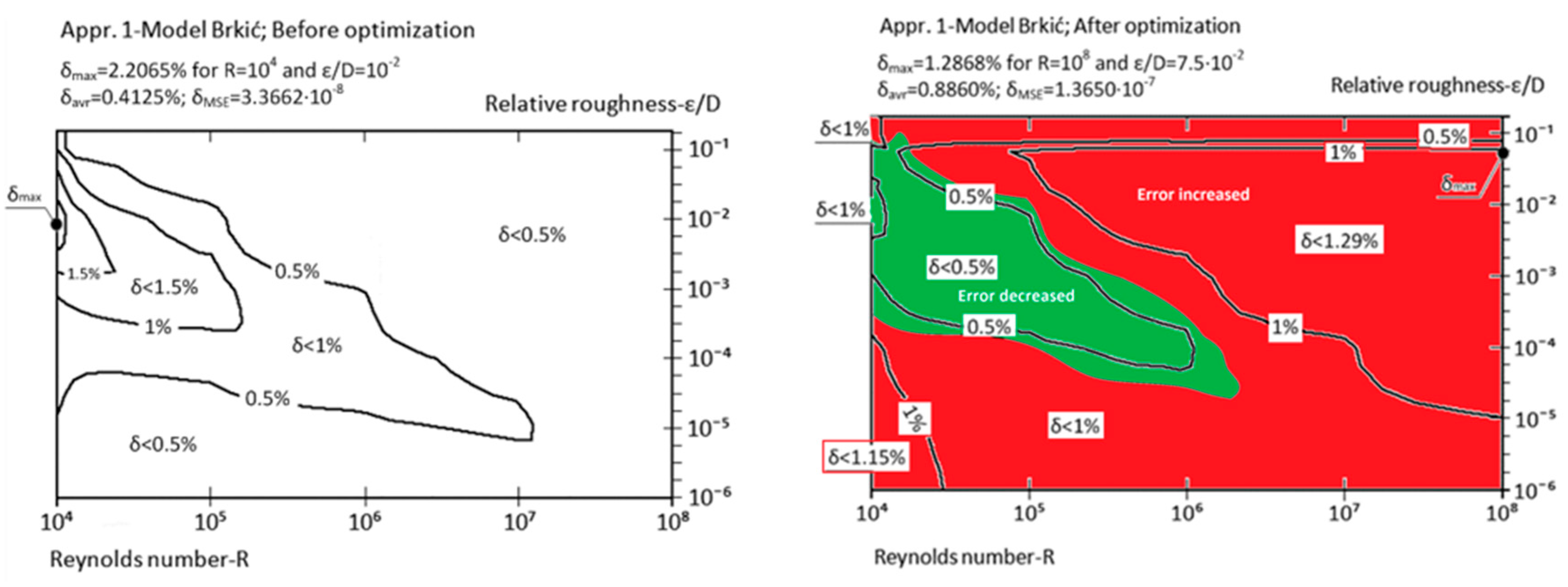
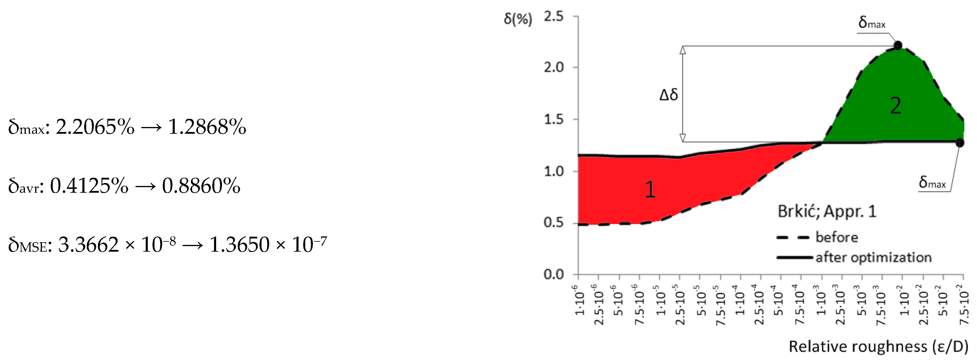
Figure 3.
Relative error before and after optimization; Brkić (Appr. 2; Equation (7)).
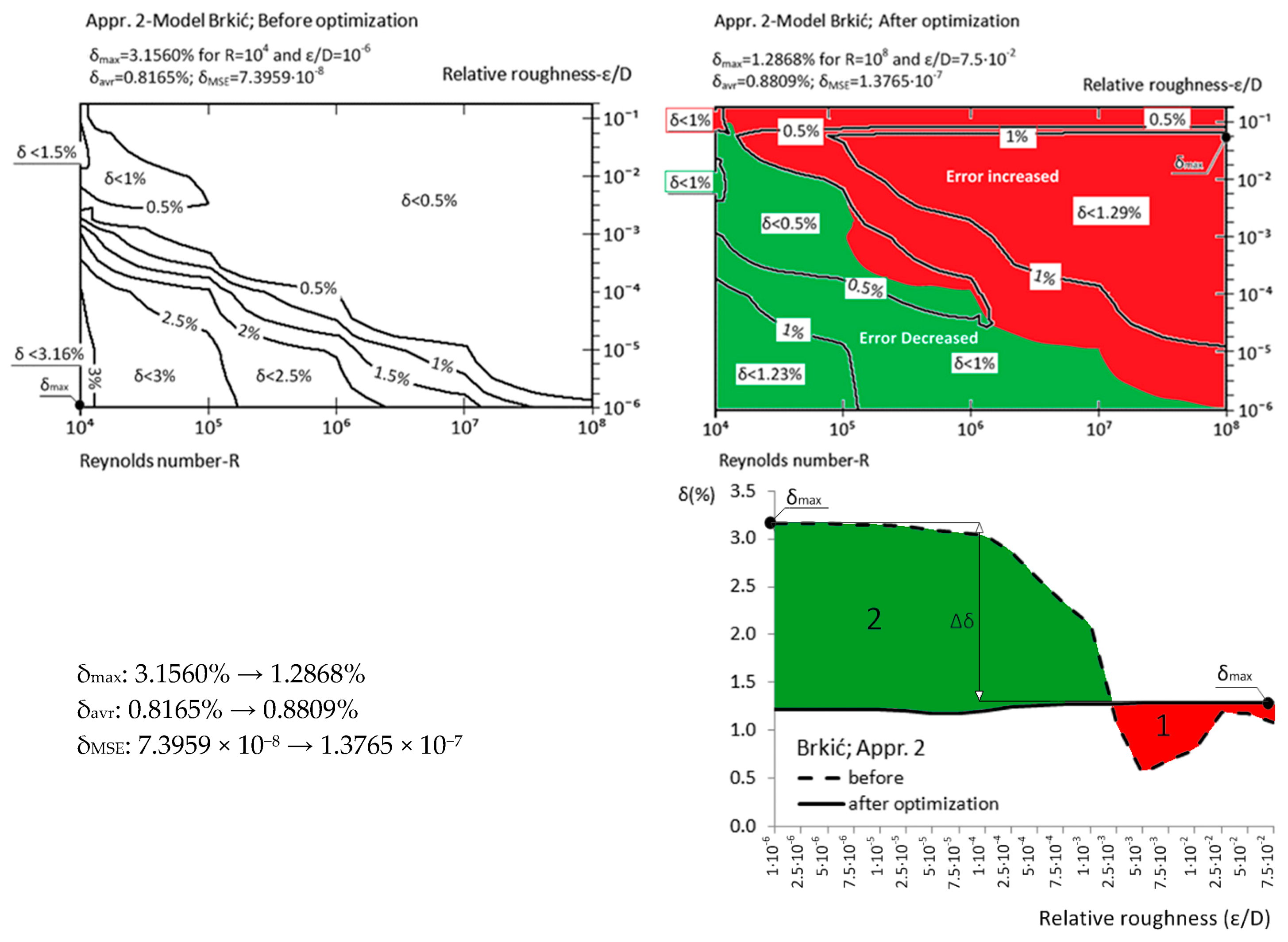
Figure 4.
Relative error before and after optimization; Brkić (Appr. 3; Equation (8)).

Figure 5.
Relative error before and after optimization; Brkić (Appr. 4; Equation (9)).
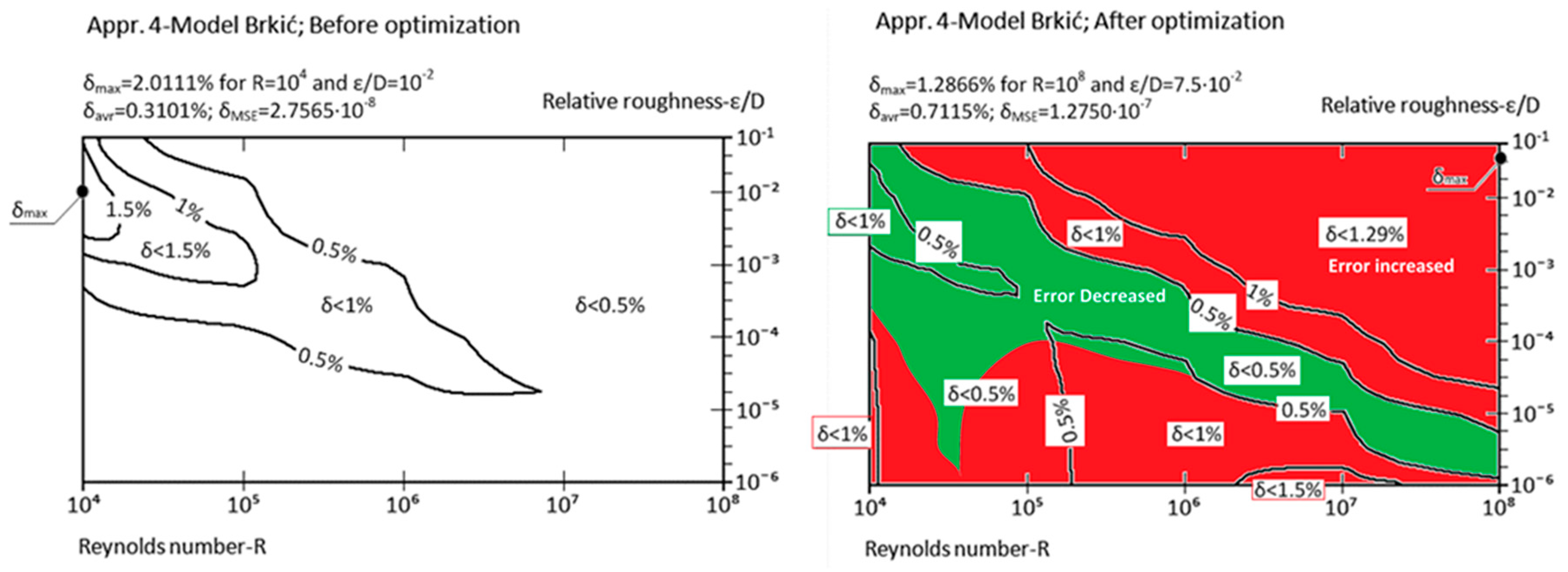
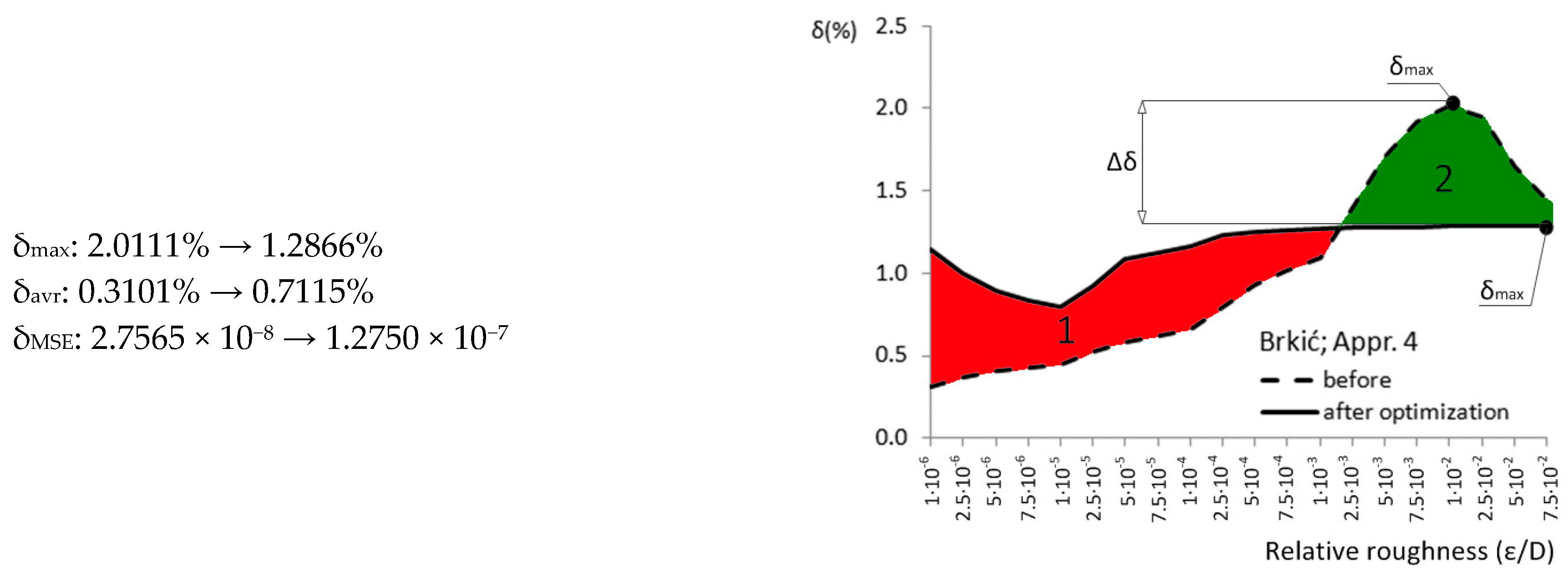
Figure 6.
Relative error before and after optimization; Fang et al. (Appr. 5; Equation (10)).

Figure 7.
Relative error before and after optimization; Ghanbari et al. (Appr. 6; Equation (11)).

Figure 8.
Relative error before and after optimization; Papaevangelou et al. (Appr. 7; Equation (12)).
Figure 8.
Relative error before and after optimization; Papaevangelou et al. (Appr. 7; Equation (12)).

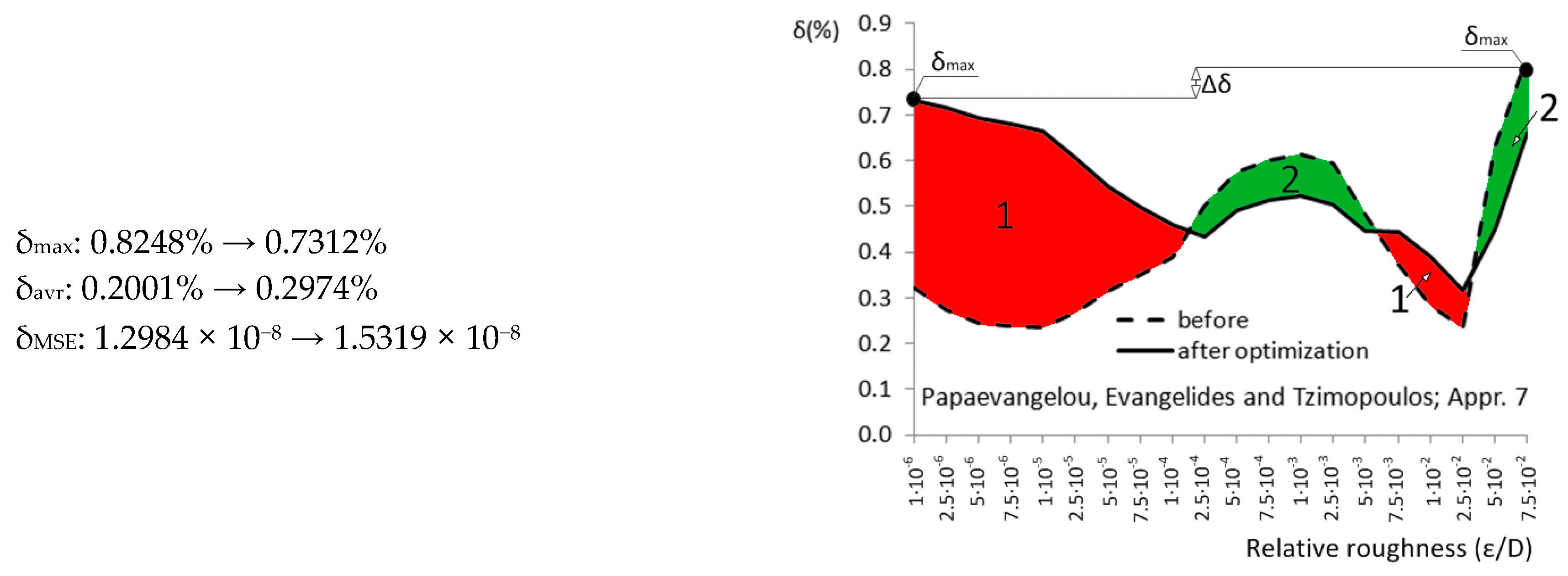
Figure 9.
Relative error before and after optimization; Avci and Karagoz (Appr. 8; Equation (13)).
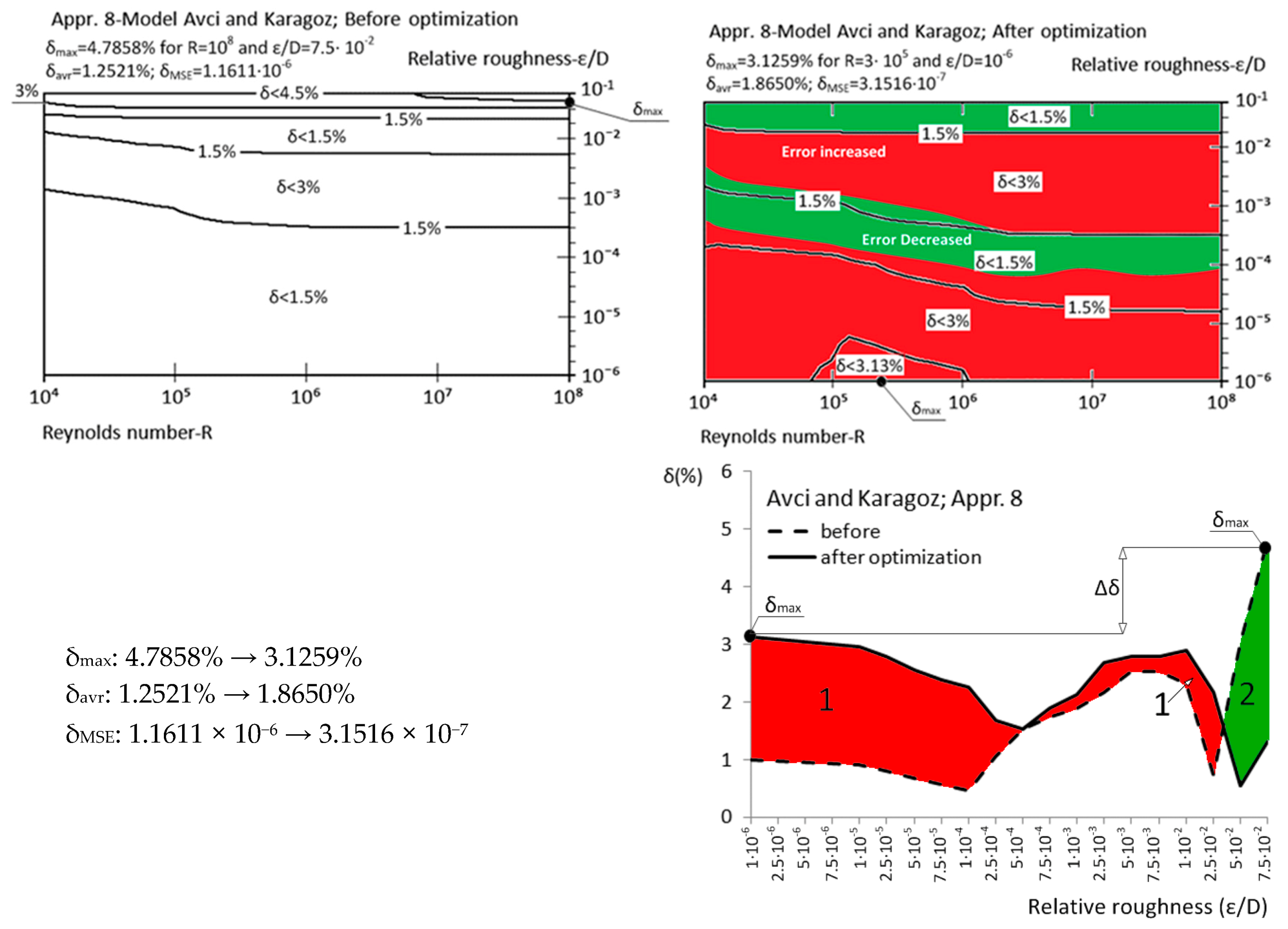
Figure 10.
Relative error before and after optimization Buzzelli (Appr. 9; Equation (14)).

Figure 11.
Relative error of Sonnad and Goudar (Appr. 10; Equation (15)) before and after optimization; optimized by Vatankhah and Kouchakzadeh [43,44].

Figure 12.
Relative error of Romeo, Royo and Monzón (Appr. 11; Equation (16)) before and after optimization; optimized by Ćojbašić and Brkić [42].
Figure 12.
Relative error of Romeo, Royo and Monzón (Appr. 11; Equation (16)) before and after optimization; optimized by Ćojbašić and Brkić [42].
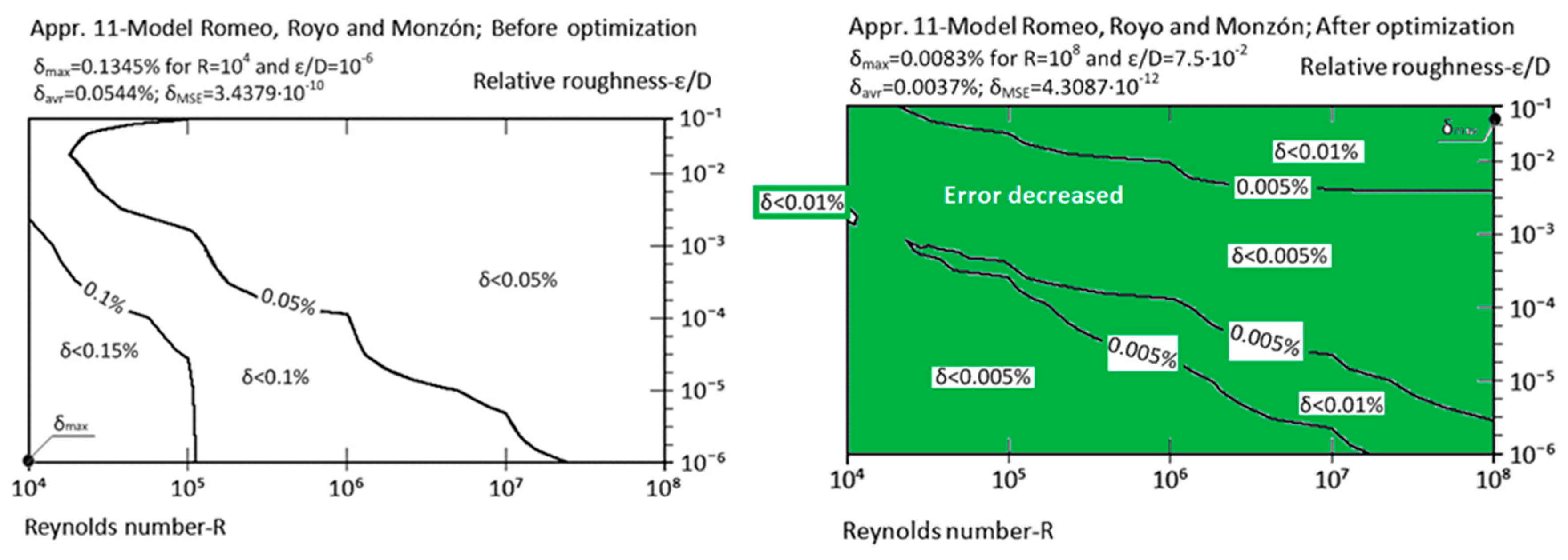

Figure 13.
Relative error before and after optimization; Manadilli (Appr. 12; Equation (17)).
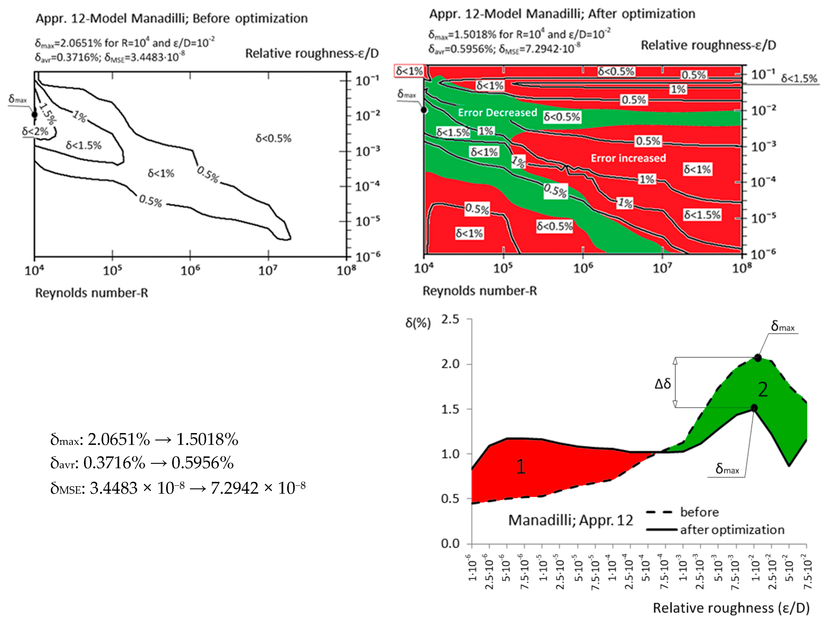
Figure 14.
Relative error before and after optimization; Chen [29] (Appr. 13; Equation (18)).
Figure 14.
Relative error before and after optimization; Chen [29] (Appr. 13; Equation (18)).
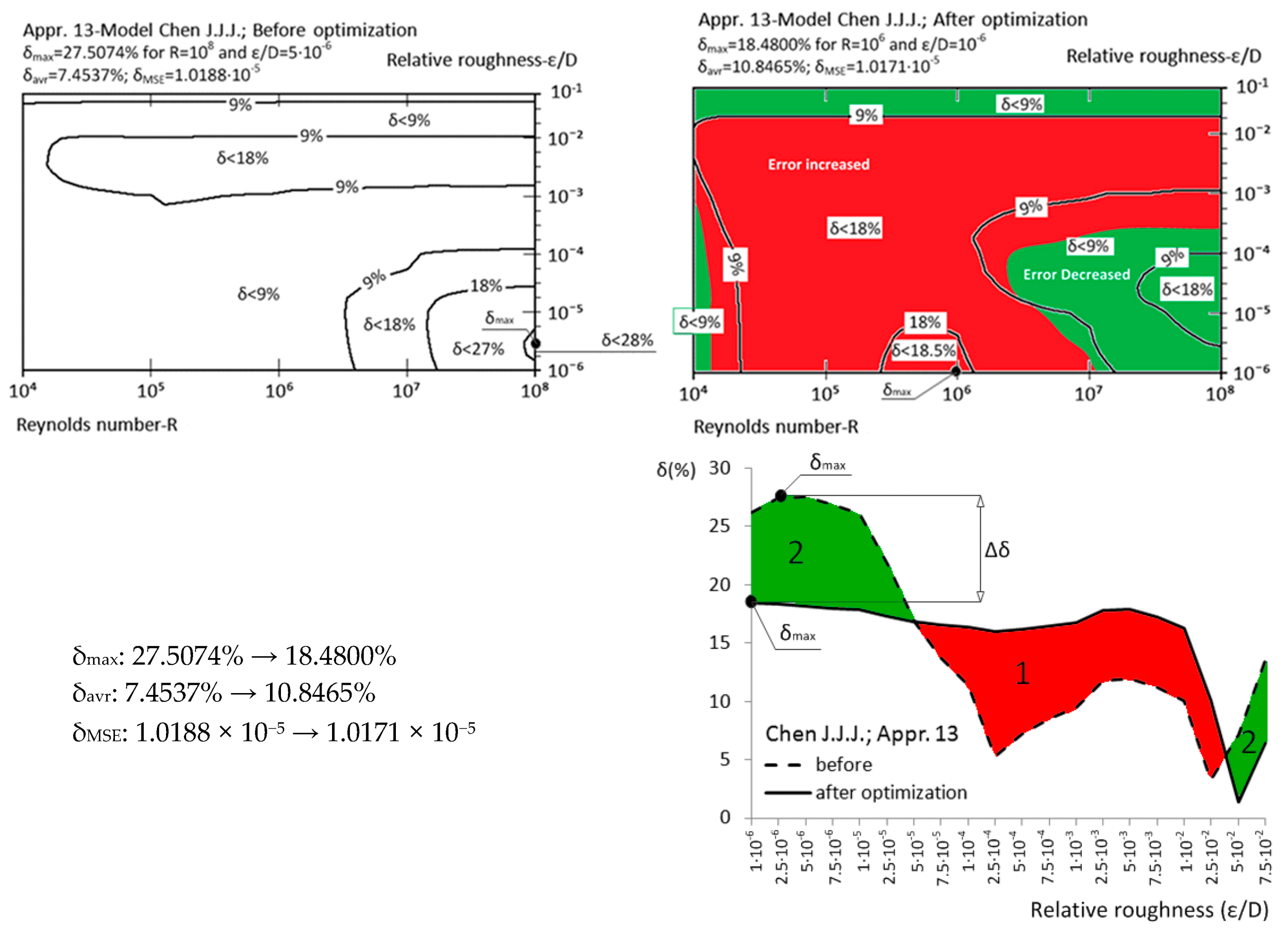
Figure 15.
Relative error of Serghides (Appr. 14; Equation (19)) before and after optimization; optimized by Ćojbašić and Brkić [42].
Figure 15.
Relative error of Serghides (Appr. 14; Equation (19)) before and after optimization; optimized by Ćojbašić and Brkić [42].

Figure 16.
Relative error of simpler version before and after optimization; Serghides (Appr. 15; Equation (20)).
Figure 16.
Relative error of simpler version before and after optimization; Serghides (Appr. 15; Equation (20)).
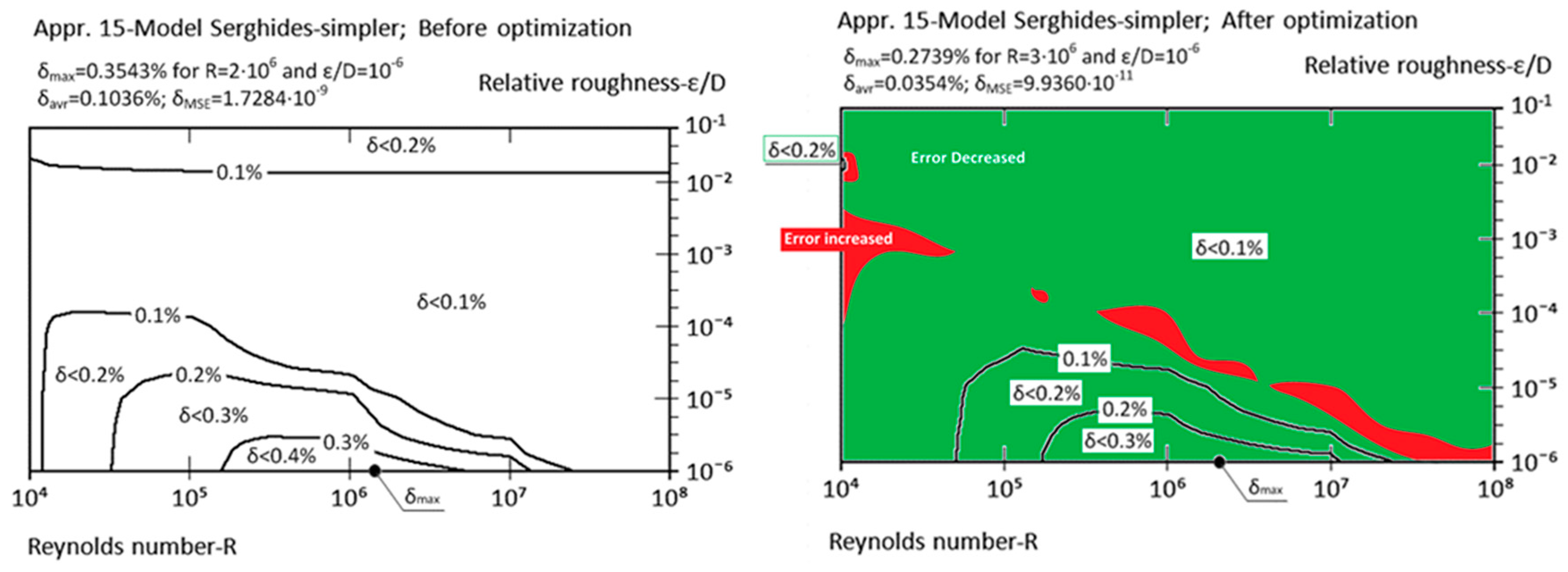
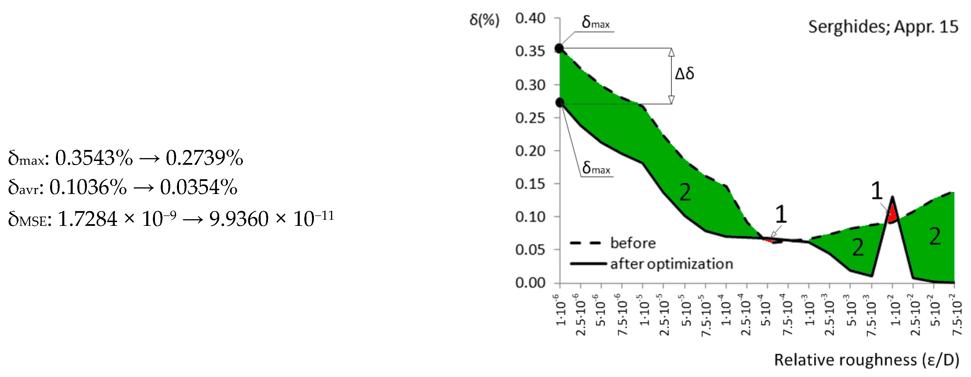
Figure 17.
Relative error before and after optimization; Haaland (Appr. 16; Equation (21)).

Figure 18.
Relative error before and after optimization; Zigrang and Sylvester (Appr. 17; Equation (22)).
Figure 18.
Relative error before and after optimization; Zigrang and Sylvester (Appr. 17; Equation (22)).
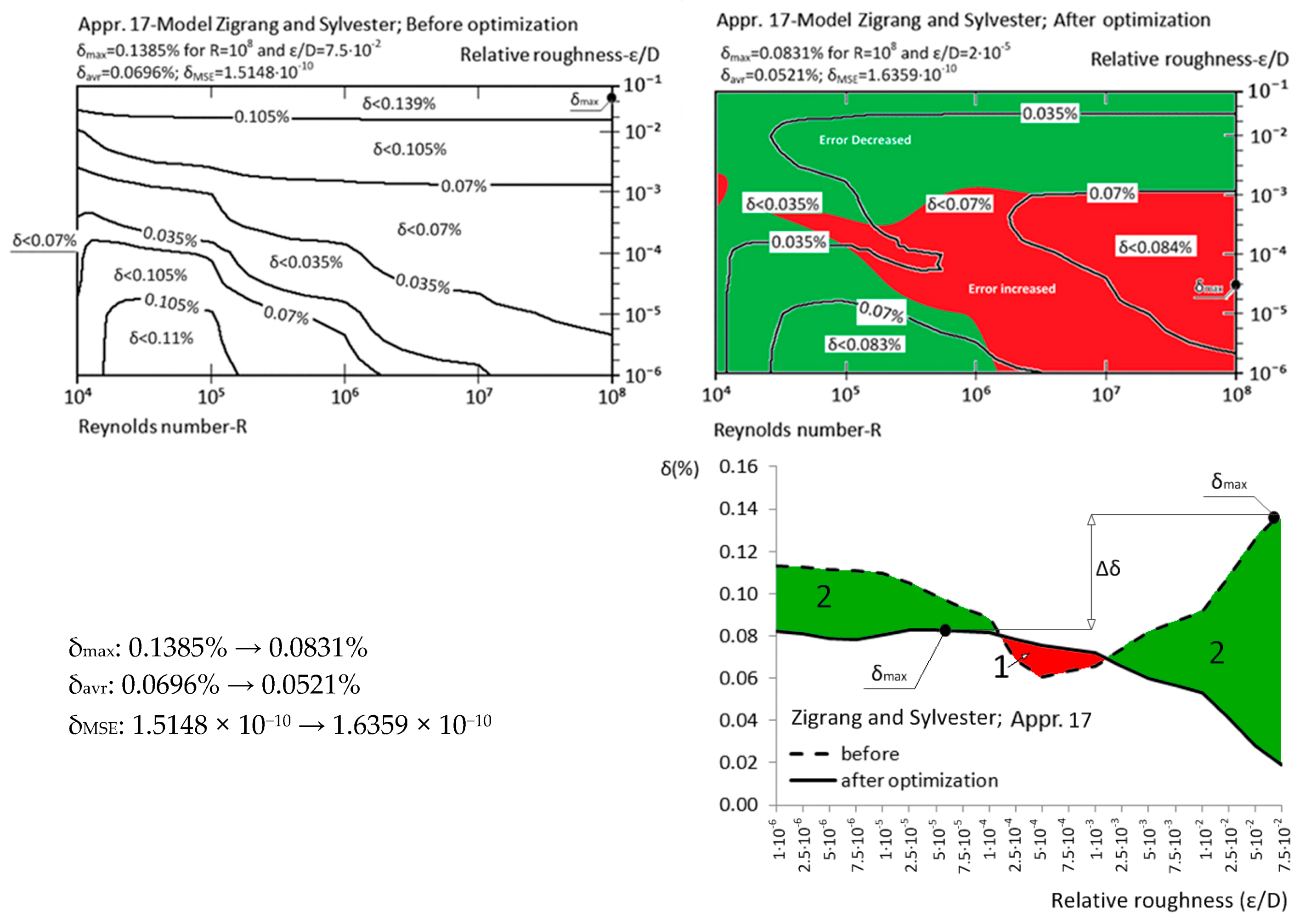
Figure 19.
Relative error of simpler version before and after optimization; Zigrang and Sylvester (Appr. 18; Equation (23)).
Figure 19.
Relative error of simpler version before and after optimization; Zigrang and Sylvester (Appr. 18; Equation (23)).

Figure 20.
Relative error before and after optimization; Barr (Appr. 19; Equation (24)).

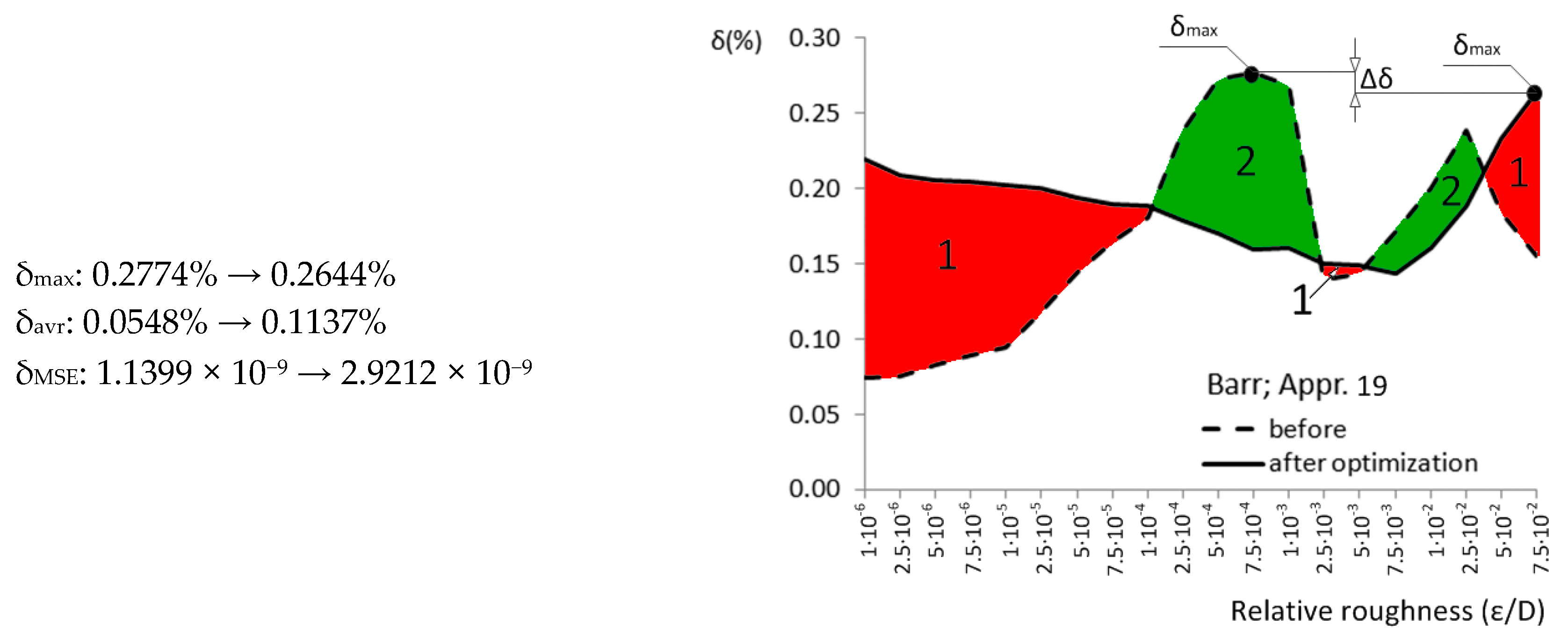
Figure 21.
Relative error before and after optimization; Round (Appr. 20; Equation (25)).
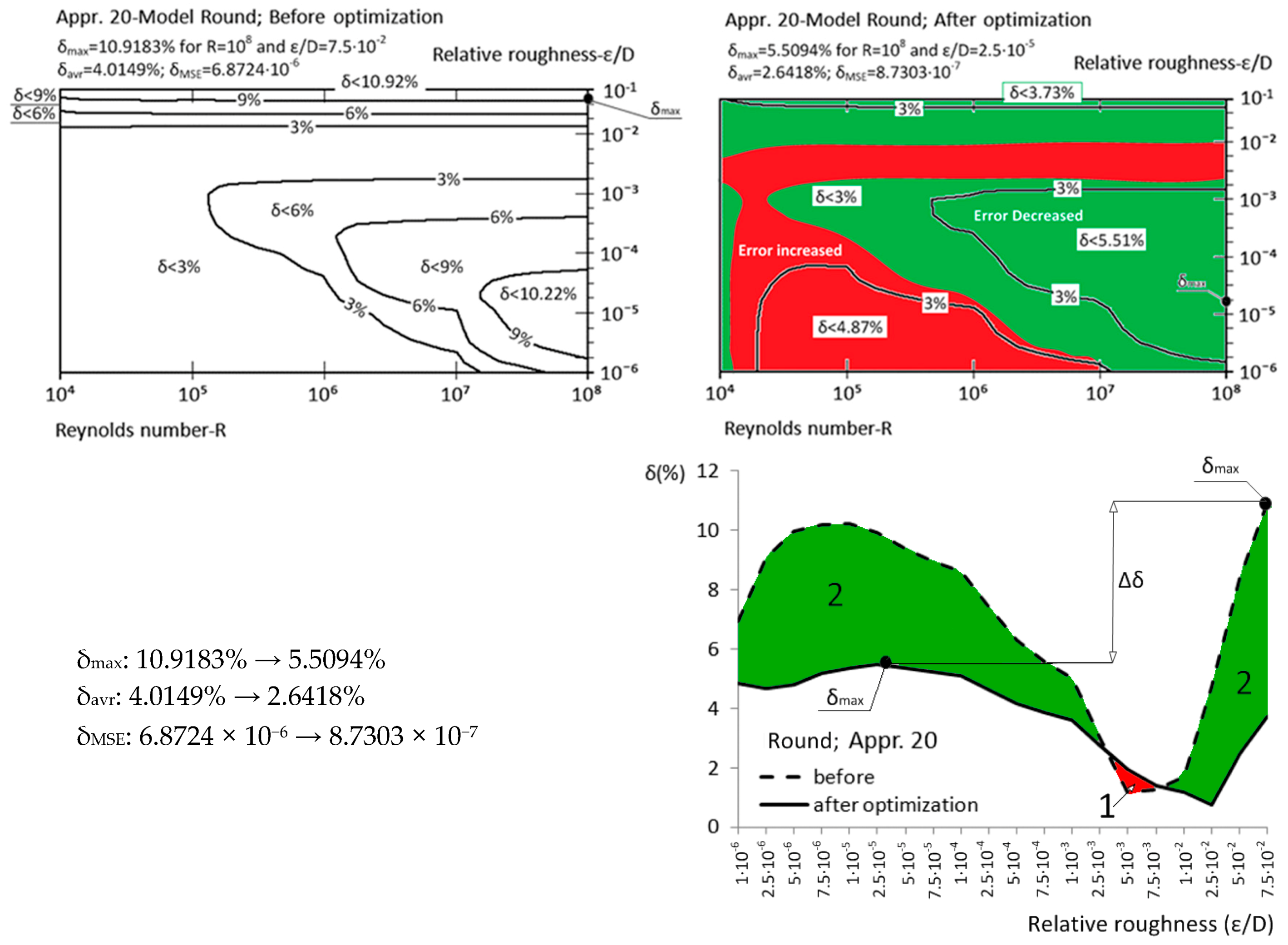
Figure 22.
Relative error before and after optimization; Chen (Appr. 21; Equation (26)).
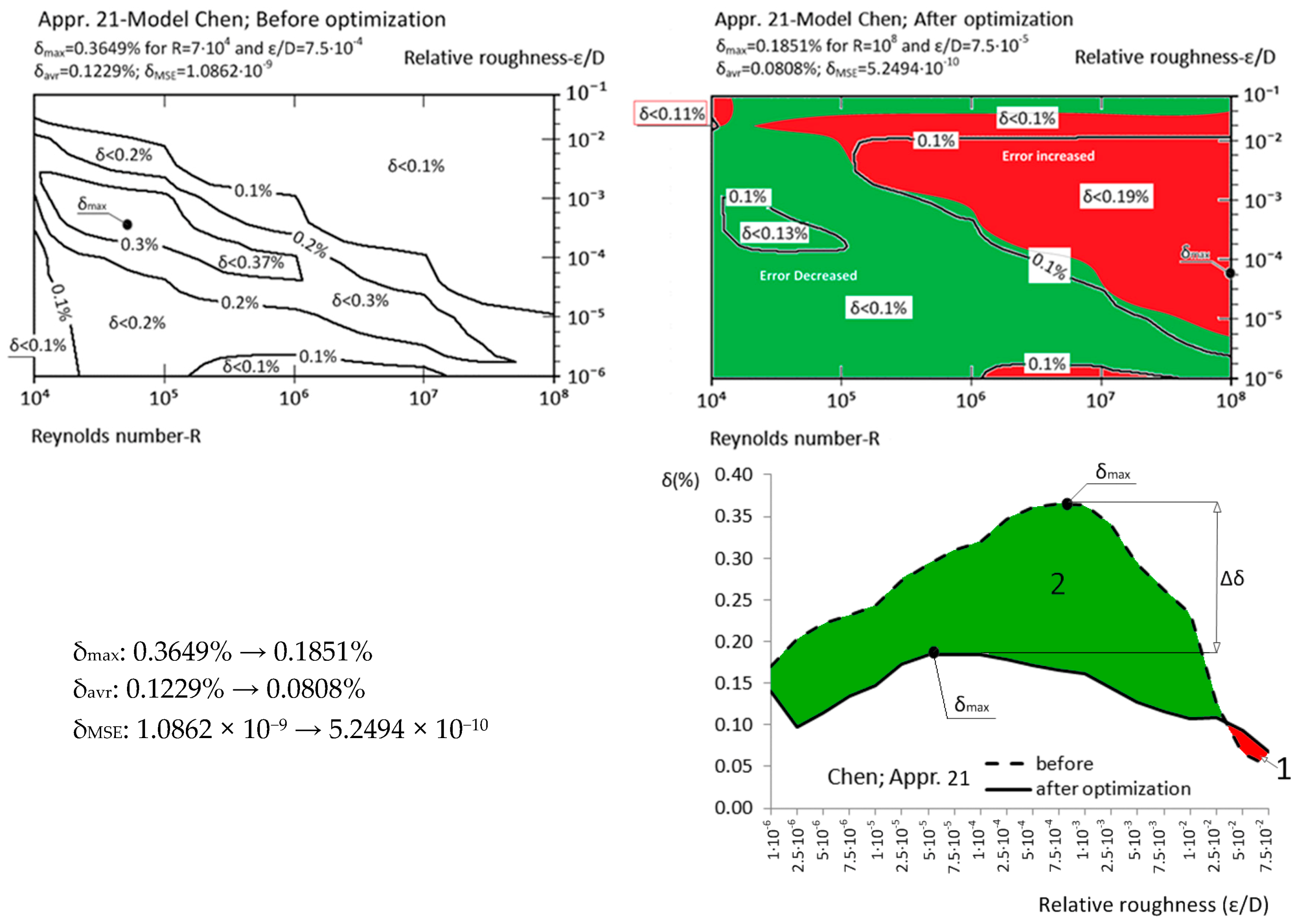
Figure 23.
Relative error before and after optimization; Swamee and Jain (Appr. 22; Equation (27)).
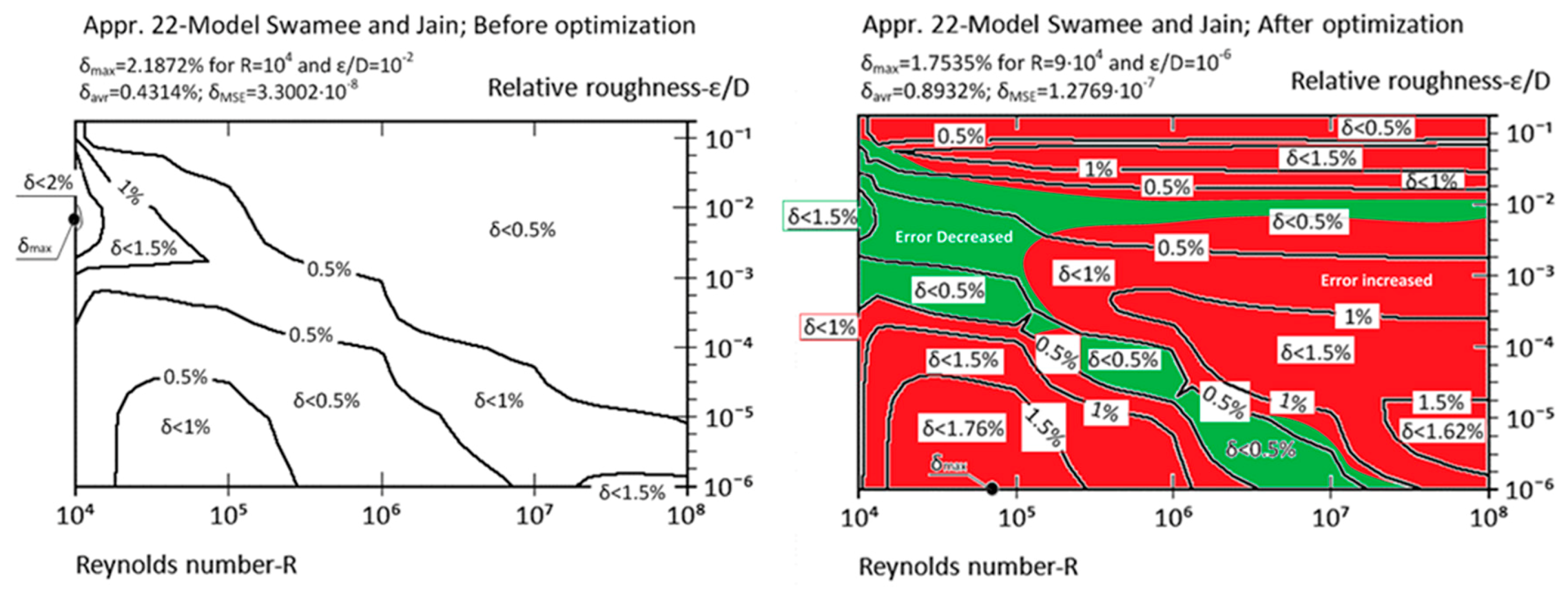

Figure 24.
Relative error before and after optimization; Eck (Appr. 23; Equation (28)).

Figure 25.
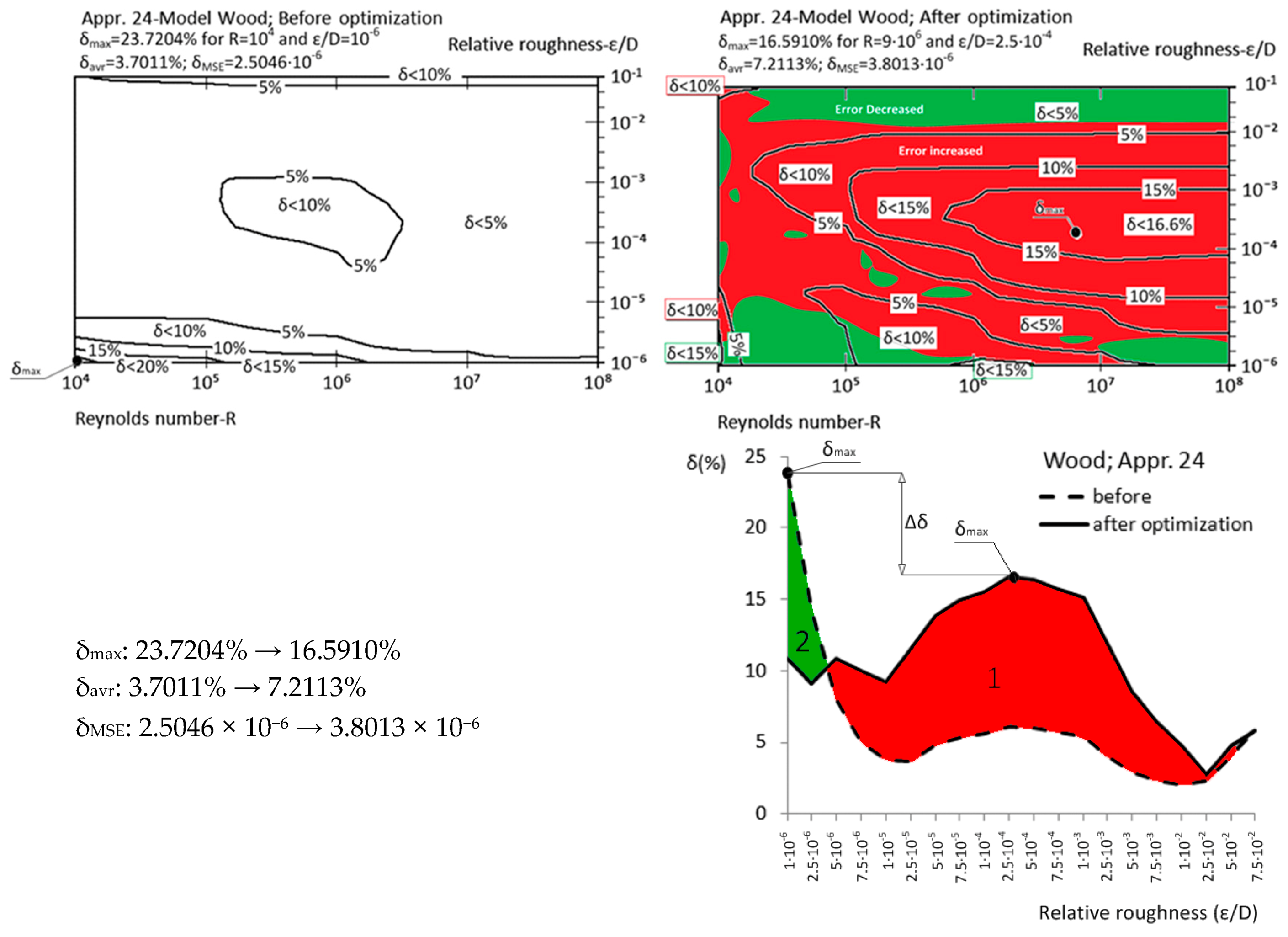
Relative error before and after optimization; Wood (Appr. 24; Equation (29)).

Figure 26.
Relative error before and after optimization; Moody (Appr. 25; Equation (30)).


Table 1.
Maximal relative error of the explicit approximations of the Colebrook–White equation before and after genetic optimization.
Table 1.
Maximal relative error of the explicit approximations of the Colebrook–White equation before and after genetic optimization.
| Approximation No. | With Original Parameters | After Genetic Optimization | Estimation of Improvement | Source |
|---|---|---|---|---|
| Appr. 11; Equation (16) | 0.1345% | 0.0083% | extremely successful | Romeo et al. [27,42] |
| Appr. 14; Equation (19) | 0.1385% | 0.0026% | extremely successful | Serghides [30,42] |
| Appr. 10; Equation (15) | 0.8007% | 0.1473% | successful | Sonnad and Goudar [26,43] |
| Appr. 2; Equation (7) | 3.1560% | 1.2871% | successful | Brkić [19] |
| Appr. 9; Equation (14) | 0.1385% | 0.0797% | successful | Buzzelli [25] |
| Appr. 15; Equation (20) | 0.3543% | 0.2739% | successful | Serghides [30] |
| Appr. 17; Equation (22) | 0.1385% | 0.0831% | successful | Zigrang and Sylvester [32] |
| Appr. 18; Equation (23) | 1.0075% | 0.7496% | successful | Zigrang and Sylvester [32] |
| Appr. 20; Equation (25) | 10.9183% | 5.5094% | successful | Round [34] |
| Appr. 21; Equation (26) | 0.3649% | 0.1851% | successful | Chen [36] |
| Appr. 1; Equation (6) | 2.2065% | 1.2868% | moderately successful | Brkić [19] |
| Appr. 3; Equation (8) | 2.0715% | 1.3326% | moderately successful | Brkić [20] |
| Appr. 4; Equation (9) | 2.0111% | 1.2866% | moderately successful | Brkić [20] |
| Appr. 5; Equation (10) | 0.6167% | 0.5669% | moderately successful | Fang et al. [38] |
| Appr. 12; Equation (17) | 2.0651% | 1.5018% | moderately successful | Manadilli [28] |
| Appr. 13; Equation (18) | 27.5074% | 18.4800% | moderately successful | Chen [29] |
| Appr. 16; Equation (21) | 1.4083% | 1.1098% | moderately successful | Haaland [31] |
| Appr. 22; Equation (27) | 2.1872% | 1.7535% | moderately successful | Swamee and Jain [37] |
| Appr. 23; Equation (28) | 8.1953% | 5.6955% | moderately successful | Eck [21] |
| Appr. 6; Equation (11) | 2.8962% | 2.5947% | not very successful | Ghanbari et al. [22] |
| Appr. 7; Equation (12) | 0.8248% | 0.7312% | not very successful | Papaevangelou et al. [23] |
| Appr. 8; Equation (13) | 4.7858% | 3.1259% | not very successful | Avci and Karagoz [24] |
| Appr. 19; Equation (24) | 0.2774% | 0.2644% | not very successful | Barr [33] |
| Appr. 24; Equation (29) | 23.7204% | 16.5910% | not very successful | Wood [39] |
| Appr. 25; Equation (30) | 21.4855% | 18.1024% | not very successful | Moody [40] |
© 2017 by the authors. Licensee MDPI, Basel, Switzerland. This article is an open access article distributed under the terms and conditions of the Creative Commons Attribution (CC BY) license (http://creativecommons.org/licenses/by/4.0/).
Share and Cite
MDPI and ACS Style
Brkić, D.; Ćojbašić, Ž. Evolutionary Optimization of Colebrook’s Turbulent Flow Friction Approximations. Fluids 2017, 2, 15. https://doi.org/10.3390/fluids2020015
AMA Style
Brkić D, Ćojbašić Ž. Evolutionary Optimization of Colebrook’s Turbulent Flow Friction Approximations. Fluids. 2017; 2(2):15. https://doi.org/10.3390/fluids2020015
Chicago/Turabian StyleBrkić, Dejan, and Žarko Ćojbašić. 2017. "Evolutionary Optimization of Colebrook’s Turbulent Flow Friction Approximations" Fluids 2, no. 2: 15. https://doi.org/10.3390/fluids2020015