Lagrangian Modeling of Turbulent Dispersion from Instantaneous Point Sources at the Center of a Turbulent Flow Channel

Abstract

The paper is focused on the simulation and modeling of the dispersion from an instantaneous source of heat or mass located at the center of a turbulent flow channel. The flow is modeled with a direct numerical simulation, and the dispersion is modeled with Lagrangian methods based on Lagrangian scalar tracking (LST). The LST technique allows the simulation of scalar sources that span a range of Prandtl or Schmidt numbers that cover orders of magnitude. The trajectories of individual heat or mass markers are tracked, generating a probability distribution function that describes the behavior of instantaneous point sources of a scalar in the turbulent field. The effect of the Prandtl or Schmidt number on turbulent dispersion is examined, with emphasis on the dispersion pattern. Results for Prandtl or Schmidt numbers between 0.1 and 15,000 are presented. For an instantaneous source at the channel center, it is found that there are two zones of cloud development: one where molecular diffusion plays a role at very small times (early stage of the dispersion), and one where turbulent convection dominates. The asphericity of the scalar marker cloud is found to increase monotonically, in contrast to published results for isotropic, homogenous turbulence, where the asphericity goes through a maximum.

1. Introduction

As turbulence is the rule rather than the exception in fluid flows, in industry as well as in the environment, a strong and ongoing effort by scientists and engineers has focused on the modeling and simulation of turbulent flows. The development of both experimental [1,2,3] and simulation techniques [4,5,6] has improved our understanding of the mechanisms of turbulence generation and dissipation [7,8,9] and as a consequence has enabled the use of computational fluid dynamics (CFD) techniques to reliably design processes and equipment where turbulence dominates. In addition, the case when a scalar is dispersed within a turbulent flow field is important in a host of applications where the flow is coupled with transport of heat or mass. Typical examples from everyday life are the dispersion of smoke and chemicals from industrial smoke stacks, agitated mixing, etc. Other examples with industrial applications are heat exchangers, industrial mixing, flow in chemical reactors and in catalyst regeneration units, heat transfer over moving blades, and the dispersion of pollutants in rivers and oceans.

While a much broader research effort has been devoted to the modeling of turbulent flow [4,5], the effort to simulate and develop models for turbulent heat transfer has been more limited [10,11,12,13,14,15,16,17]. The simulations are mainly divided into two categories: those that are based on the Eulerian approach to describing transport phenomena (and where the system of reference is not moving), and those that are based on the Lagrangian approach to transport phenomena (where the system of reference moves with the scalar being dispersed).

Eulerian techniques are employed by typical CFD software packages. In these, models that are by-and-large based on the Reynolds analogy for heat or mass transport in turbulent flows are utilized. These models typically are based on the concepts of eddy diffusivity, the mixing length, the turbulent kinetic energy, and the rate of turbulence dissipation. Models based on the Reynolds analogy make the assumption that the eddy diffusivity of a scalar is related to the eddy viscosity for the flow through a form of the turbulent Prandtl number (Pr_t). Such models are empirical and require the calibration of several variables with experiments. They often fail to produce accurate results, for example in asymmetric flows, like the flow between a rough and a smooth plate, or transfer in annular flow [18]. Other models include those that are based on heat transfer equations that are analogous to the k-ε models suffer from the same shortcomings as the k-ε models for flow [17]. Second moment closure models, such as the analogues of Reynolds Stress Models for heat transfer, require the modeling of a large number of terms in the scalar flux transport equations and in the turbulent stress equations, which are difficult to measure experimentally (i.e., the terms of the pressure-strain term, and the turbulent dissipation term) and are known to be inaccurate close to solid boundaries [19,20,21]. In wall turbulence, where a solid boundary is present, the Reynolds analogy–based models fail because of a fundamental reason: the scales of turbulence that contribute to scalar transport are not the same as the scales that contribute to heat or mass transport, and the later depend on the Prandtl number (Pr) of the fluid [22,23,24,25,26]. (Note that from now on, we use terminology that can be applied to heat transfer and the Prandtl number, while the results and analysis apply to mass transfer and the Schmidt number.).

Lagrangian techniques have also been employed for the study of turbulent transport, but mostly for developing theoretical understanding. In isotropic, homogeneous turbulence, such simulation techniques have been very successful in exploring the stochastic modeling of turbulence over a range of Pr between 0.04 and 1024 [27,28,29,30,31,32,33], while in anisotropic wall turbulence, they have been used to describe transport over a range of Pr that covers six orders of magnitude (from Pr = 0.01 to Pr = 50,000) and different modes of heat transfer [34,35,36]. Hybrid Eulerian-Lagrangian methods have also been recently utilized [37]. An advantage in terms of computations for Lagrangian methods is the ability to simulate heat transfer cases with practically no limits on the Pr. Eulerian direct numerical simulation methods are limited not only to relatively low Reynolds numbers (Re), but also to a narrow range of small and intermediate Pr. This limitation arises because, in order to resolve all the scales of motion and temperature [38], the number of computational mesh points has to be proportional to Pr^3/2Re^9/4. An increase of Pr by one order of magnitude means an increase of the number of grid points by about thirty times. The main disadvantage of Lagrangian methods is the need to use a large number of scalar markers to simulate turbulent transfer and the slow convergence of particle-based methods [39].

In the present work, Lagrangian scalar tracking (LST) is used to investigate turbulent dispersion from instantaneous point sources of a scalar at the middle of a turbulent flow channel simulated with a direct numerical simulation (DNS). (The cloud of scalar markers resulting from an instantaneous point release is usually called a puff). The DNS method has been employed and validated with experiment results in Poiseuille and Poiseuille-Couette flow [40], while LST simulation results have been found to agree well with different experimental results for heat or mass transfer [41]. The significant advantage of the LST, in terms of physics, is the ability to release such particle puffs that form the most elementary unit for heat transfer. The heat markers in the puff can be followed individually and can be correlated with actual flow structures [25,26]. The contributions of this work are (a) to describe the computational method utilized to develop the LST results, (b) to investigate the characteristics of turbulent transport in a channel flow and its comparison to turbulent dispersion in an isotropic turbulent field, and (c) to explore possible Pr effects on turbulent dispersion, with the use of results for Pr = 0.1, 6, 100, 2400, and 15,000, which correspond to liquid metals, gases, liquids, and heavy oils.

2. Results

2.1. Statistics of the Marker Location and Prandtl number (Pr) Effects

The friction Re for the presented simulation results is Re_τ = 300. Figure 1 is a plot of the mean streamwise position of the puffs that result from the release of 10,000 particles at an instant at a point source located at the middle of the turbulent flow channel at x₀ = 0 and y₀ = 0. The time of particle release is t₀ = 0. All space and time quantities presented in this study are in viscous wall units. The bottom wall of the channel is considered to be at y = −300 and the top wall at y = 300. The mean puff position does not change significantly with the Pr, as expected.

While the first order statistics of the puff location are not expected to change with Pr, the second order statistics can be a better measure to show the Pr effects on the puff motion, especially at small times since the scalar marker release. In Figure 2 we present the second order statistics of the puff motion in the three spatial directions as a function of the time elapsed from the release of the puff. The variance of the distribution of the location of the markers in each cloud and at each time is calculated as follows:

$${\mathrm{\sigma }}_X={\overline{{\left(\overline{X}-X\right)}^2}}^{1/2},{\mathrm{\sigma }}_Y={\overline{{\left(\overline{Y}-Y\right)}^2}}^{1/2}\mathrm{and}{\mathrm{\sigma }}_Z={\overline{{\left(\overline{Z}-Z\right)}^2}}^{1/2}$$

(1)

where the overbar designates average over all the markers in the flow field, and X, Y, and Z are the locations of markers in the x, y, and z directions.

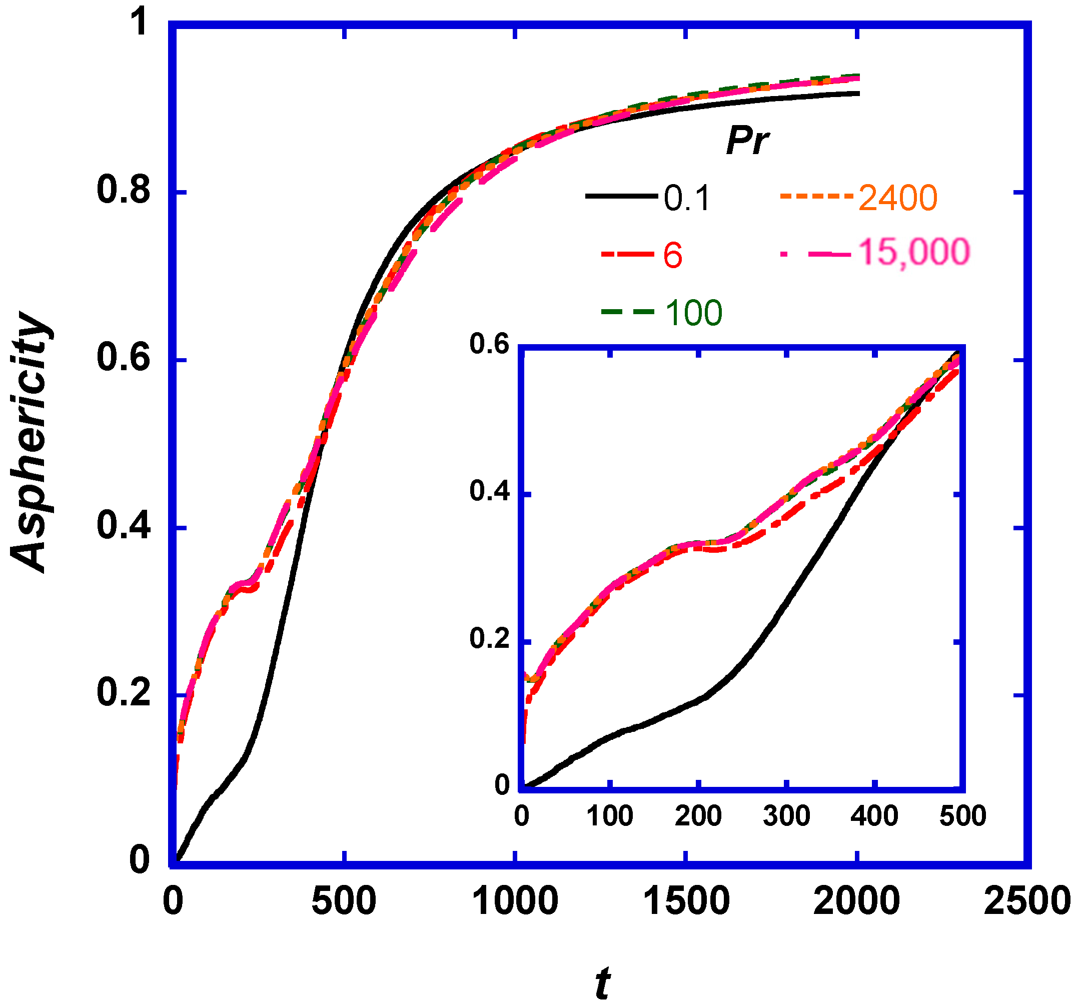
2.2. Shape of Puff and Differences from Puffs Released in Isotropic Turbulence

The shape of the puffs in anisotropic turbulence is expected to be changing in the three dimensions, starting from a spherical shape and changing to a spheroid as a function of time and Pr. In isotropic turbulence, the flow and molecular effects would result in spherical puffs irrespective of Pr. Figure 3 is a depiction of the marker puff at time t = 2000 after the puff release. It is seen that the puff extends longer in the x direction at higher Pr, in agreement with Figure 2a.

A measure of the departure of the puff shape from the spherical shape is the asphericity (A_s), which can be used to quantify the deformation of a puff from a spherically symmetric geometry [42,43]. Asphericity of a body varies from 0 to 1 (A_s = 0 for a perfectly spherical cloud; A_s = 0.25 for a two-dimensional circle without width, a disc; and A_s = 1 for an infinite cylinder) [44]. The values of A_s were calculated from the moment of inertia tensor (T) of each puff [44],

$$A_s=\frac{{\left(R_1^2-R_2^2\right)}^2+{\left(R_2^2-R_3^2\right)}^2+{\left(R_3^2-R_1^2\right)}^2}{2R_g^4}$$

(2)

$$T_{ij}=\frac{{\sum }_{m=1}^N\left(S_{im}-S_i^{CM}\right)\left(S_{jm}-S_j^{CM}\right)}{N}$$

(3)

where N is the total number of markers in the puff, $R_1^2$, $R_2^2$, and $R_3^2$ are the three eigenvalues of the tensor T (i.e., the three principal radii of gyration squared for all Nmarkers), $S_{im}$ is the position of marker m in the i-th Cartesian dimension (i denotes x, y, or z), and $S_i^{CM}$ is the center of mass of the N markers in coordinate i. The puff asphericity can be seen in Figure 4 for the puff cases simulated herein.

3. Discussion

For a puff released at the channel center, one would expect that the mean puff velocity (the slope of the lines in Figure 1) would be very close to the mean flow velocity at the channel center (which is 19.15 in the simulation) at small times after the particle release. As the time elapses, the puff of markers should disperse in the vertical and spanwise directions and would eventually extend to cover the channel width. From that point and on, the mean puff velocity would be very close to the bulk velocity of the fluid in the channel. In Figure 1, it is seen that the slope of the mean streamwise position of the puff is $\frac{d\overline{X}}{dt}=19.1$ for times less than t = 500, and the slope of the line changes to $\frac{d\overline{X}}{dt}=16.7$ as times t > 1500. The change in slope, occurring between time t = 500 and t =1000, is the same for all cases of Pr. The average Y and Z positions (not shown here) remain $\overline{Y}$ = 0 and $\overline{Z}$= 0, since the turbulent channel flow is symmetric around the center plane regarding the statistics of the flow. There is no reason for the markers in the puff to move on average toward the top or toward the bottom of the channel.

Scalar dispersion is dominated by molecular effects at very small times and then by turbulent effects at longer times. In the particular case of flow in a channel examined here, the cloud of markers that comprise a puff will eventually distribute uniformly across the channel. It is expected that at long times, the standard deviation of the particle location in the y direction will be that of a uniform distribution in the y direction. The value of ${\mathrm{\sigma }}_Y$ increases and it is expected to tend to the constant value of (600²/12)^1/2 = 173.2 for all Pr, (which is the standard deviation for a uniform distribution between the values −300 and 300). It takes somewhat longer for higher Pr markers to get to this predicted value because at small times, there is a molecular diffusion effect. While the marker cloud extends in the normal direction, markers start to enter the log layer and then the viscous wall region closer to the channel walls. When this occurs, the effects of the Pr become more important and manifest themselves in the values of ${\mathrm{\sigma }}_X$. When high Pr markers enter the near wall region, the molecular motion is rather limited, and it is more difficult for them to jump out of that region with molecular means (contrary to low Pr markers that can jump out of the near wall region because of turbulent velocity fluctuations and also because of molecular motion). In this respect, higher Pr markers stay longer in the viscous wall region, where the mean streamwise velocity is smaller than the bulk fluid velocity, and the high Pr clouds tend to extend longer in the x direction. This is seen in Figure 2a by observing the slope of the ${\mathrm{\sigma }}_X$ line that increases for high Pr puffs. The existence of slower moving markers is also seen in Figure 3, where the individual markers trailing at the edge of the puffs for Pr = 100 and Pr = 15,000 are seen.

Regarding the puff shape, all of the puffs started as sphere-like at very small times, but changed their shape at larger times (see Figure 4). Intermediate and high Pr puffs (Pr ≥ 6) have almost the same asphericity as time elapses, but the low Pr puff exhibits differences at times up to t = 400. The reason for these differences, and the reason that the Pr = 0.1 puff is shaped almost like a sphere for a longer time, is the high molecular diffusion of this puff relative to the others. Due to the random Brownian motion, the markers are initially like particles within the volume of a balloon that expands with time. At larger times, the markers start to enter the logarithmic region and the viscous wall region, and the puff starts to elongate, departing from the spherical, balloon-like shape. Recent results about the asphericity and the puff shape of passive particles released in isotropic, homogeneous turbulence [45], indicate that the marker puffs start as spherical and quickly deform into elongated structures, showing a maximum value of asphericity of about 0.7 within 13 Kolmogorov time scales. Beyond that point, the puffs tend to slowly return to a more spherical shape with asphericity values close to 0.2 at longer dispersion times, longer than the eddy turnover time scale. This is a notable difference with the present case, where the deformation of the shape of the puff is not reversible.

In prior work about the dispersion of a puff released at the wall of a turbulent flow channel, it has been found that there are three zones of puff development, depending on the physical mechanism that dominates dispersion [46]. Zone I is dominated by molecular diffusion effects, Zone II is a transition zone where both molecular and convection effects are important, and Zone III is the zone where turbulent convection is dominant. The time that it takes for a puff to transition between these zones depends on the Pr. For example, Pr = 0.1 puffs were found to exit Zone I at about t = 20, while Pr = 2400 puffs would exit this zone at t = 200. In the present case, where the puffs are released in the center of the channel, there appear to be only two Zones of puff development. Zones I and II (where molecular effects can be important) are very short for Pr ≥ 6. When the beginning of Zone III is identified as the time period in which the asphericity becomes larger than 0.1, the transition to turbulent convection dominance does not take more than t = 5. Only for Pr = 0.1, the asphericity stays below 0.1 for times up to t = 150. A prior study for dispersion from the center of a channel flow also indicated that Pr effects are more important for low Pr dispersion (Pr on the order of one and lower) [47]. However, that study was for a Re_τ = 150 channel, where the convective effects are less prominent than in the current study, and it was limited to dispersion up to time t = 125.

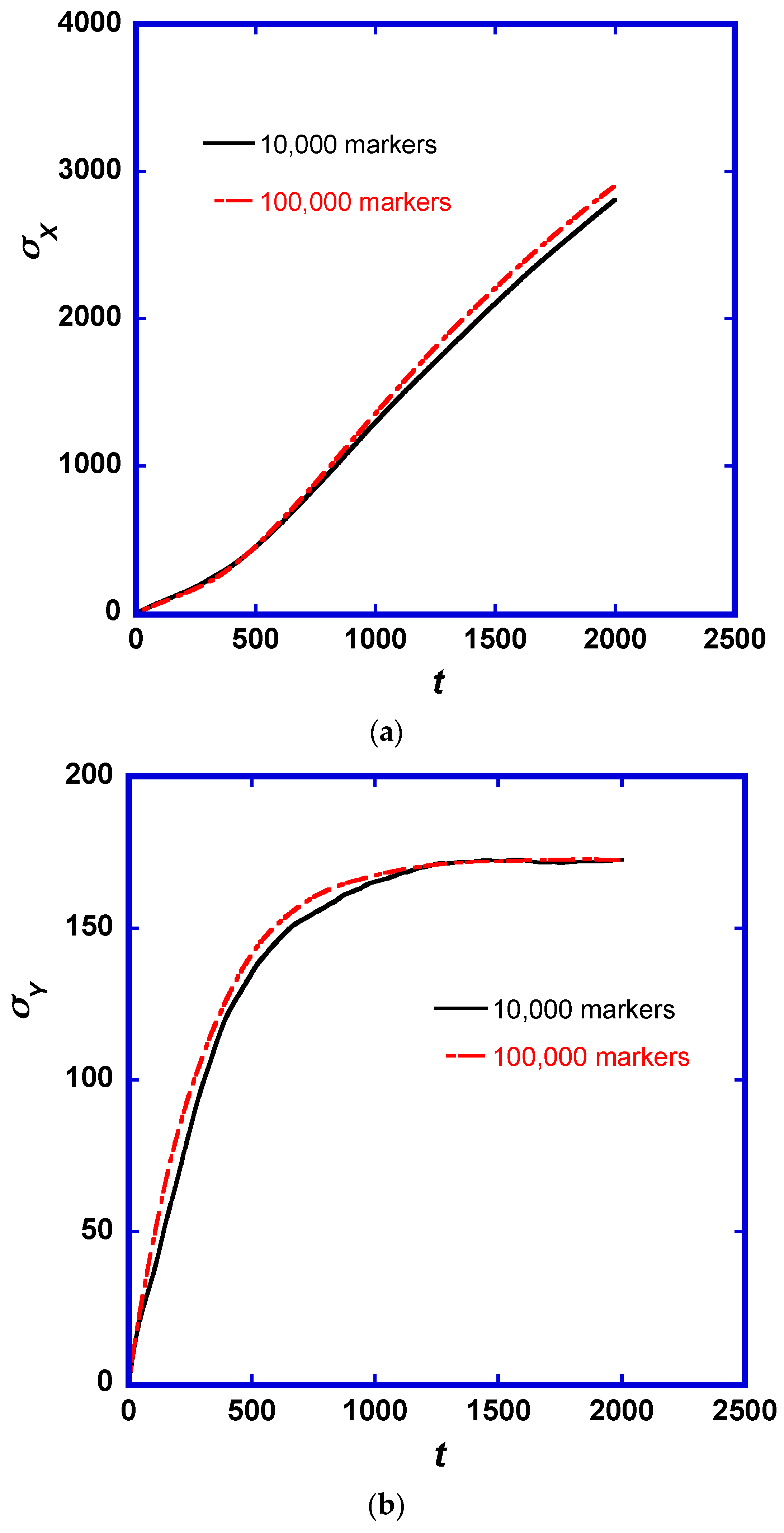
4. Materials and Methods

The velocity field for a Newtonian and incompressible fluid is calculated using a DNS of fully developed turbulent flow in a plane channel. The dimensions of the computational box in the x (streamwise), y (wall-normal) and z (spanwise) directions are 16 πh × 2 h × 2 πh with a half channel height (h) of 300. The flow is driven by a constant mean pressure gradient. For the present problem, the simulation is conducted on a 1024 × 129 × 256 mesh in the x, y, z directions, respectively, with uniform spacing in the x and z, while Chebyshev polynomial collocation points are used in the wall normal direction. The DNS algorithm is based on the pseudospectral method published in [10,48]. The integrity of this method has been verified with comparisons to experiments at an equal Re [49]. The Reynolds number, Re, defined with the centerline mean velocity and half channel height, h, is 5760, corresponding to a Re defined based on the hydraulic radius of ~23,000 (this is the equivalent Re for flow in a pipe). The friction Reynolds number is Re_τ = h = 300. The variables presented are dimensionless with the use of the friction velocity, u*, and the kinematic viscosity of the fluid, ν, namely, the viscous wall units. The friction velocity is given as u* = (τ_w/ρ)^1/2, where τ_w is the shear stress at the wall and ρ is the fluid density. The assumptions of no slip and no penetration are used as boundary conditions on the wall, and the heat production by viscous dissipation is assumed to be negligible. The time step was 0.1 in viscous wall units, and the iterations were carried out for 20,000 time steps for stationary channel flow in order to simulate 2000 viscous time units of flow after a puff is released. Briefly, the DNS solves the rotational form of the dimensionless Navier-Stokes equations,

$$\frac{\partial \overrightarrow{U}}{\partial t}=\overrightarrow{U}\times \overrightarrow{\mathsf{\Omega }}-\nabla \mathsf{\zeta }+\frac{1}{h}\overrightarrow{i_x}+{\nabla }^2\overrightarrow{U}$$

(4)

where $\overrightarrow{U}$ is the velocity vector, $\overrightarrow{\mathsf{\Omega }}$ is the vorticity vector, and $\overrightarrow{i_x}$ is the unit vector in x direction. The continuity equation also applies,

$$\nabla ·\overrightarrow{U}=0$$

(5)

and

$$\mathrm{\zeta }=p^{\prime }+\frac{1}{2}\overrightarrow{U}·\overrightarrow{U}$$

(6)

where the term $p\prime$ is the fluctuating component of the pressure in viscous wall units. The velocity is expanded in truncated Fourier series in the x and z directions, and a truncated Chebyshev polynomial series in the y direction. The boundary conditions in the x and z directions are periodic with periodicity length the size of the computational channel in each one of these directions. The Navier-Stokes equations are integrated in time using the pseudospectral fractional step method originally developed by Orszag and Kells [50] and the added correction suggested by Marcus [51] to correct with the pressure at the channel walls.

The trajectories of heat or mass markers released from a line parallel to the z axis at the center of the channel are calculated in the flow field created by the DNS. The total number of markers is 10,000 for each case of Pr, for a total of 50,000 markers. Since the flow is homogeneous in the z direction, it is not statistically important where on the line the markers are released, so in order to reduce the possible effects of releasing the markers in an idiosyncratic flow structure, the markers were released uniformly spaced on the line source. However, in order to obtain the statistics of the cloud location in the z direction, the z coordinate of each particle was determined after subtracting the z coordinate at the marker point of release. The flow field used for the Lagrangian scalar tracking of the markers is the same for all Pr cases, so that the effects of the Pr can be observed rather than the effects of the flow. The tracking of the passive scalar markers was based on the Kontomaris et al. [52] algorithm. The motion of the scalar markers is decomposed into a convection part and a molecular diffusion part. The convective part can be calculated from the fluid velocity at the particle position, so that the Lagrangian velocity at time t of a marker released at location $\overrightarrow{X_o}$ is assumed to be the same as the Eulerian velocity at that particle’s location at the beginning of the convective step, i.e., $\overrightarrow{V}(\overrightarrow{X_o},t)=\overrightarrow{U}[\overrightarrow{X}(\overrightarrow{X_o},t),t]$. The equation of particle motion then is

$$\overrightarrow{V}(\overrightarrow{X_o},t)=\frac{\partial \overrightarrow{V}(\overrightarrow{X_o},t)}{\partial t}$$

(7)

The effect of molecular diffusion is simulated by adding a random movement on the particle motion at the end of each convective step. A similar method was used in simulating the random diffusion part of Lagrangian trajectories in [52]. This random motion is a random jump that takes values from a Gaussian distribution with zero mean and standard deviation $\mathrm{\sigma }=\sqrt{2\mathsf{\Delta }t/Pr}$, where Δt is the time step of the simulation in viscous wall units, (Δt = 0.1). The particle velocity is found by using a mixed Lagrangian-Chebyshev interpolation between the Eulerian velocity field values at the surrounding mesh points. The particle position integration in time is approximated with a second order Adams-Bashforth scheme [53].

As previously mentioned, Lagrangian methods require a large number of scalar markers to simulate turbulent transport. In this study, 10,000 scalar markers were released on a single line source. The question of whether one needs to increase the number of markers for higher accuracy is explored by comparing results in this study with second order statistics from another numerical experiment, which was conducted with 100,000 markers and Pr = 6 being released at several line sources along the streamwise direction. While the mean marker position did not show any differences in the streamwise direction (as expected), the second order statistics exhibit some differences. The standard deviation of the scalar marker location in the streamwise and wall normal direction of Pr = 6, with 10,000 and 100,000 markers, is plotted in Figure 5. It is seen that using 100,000 markers results in about 3.5% difference in σ_x at t = 2000 and about 4.4% difference for σ_y at t = 500 (the differences disappear at long times for σ_y). However, these small differences in the second order statistics are not large enough to change the qualitative findings of the present study or to change significantly the quantitative findings about the asphericity of the particle clouds. Other simulations with a higher number of particles could benefit the accuracy of the quantitative findings herein.

5. Conclusions

A Lagrangian method to explore the dispersion of passive scalars in turbulent flow is described. The advantages of using this numerical method to model heat or mass transfer is that one can use a single velocity field obtained by running a DNS once to model the dispersion of scalars of several different Pr. In addition, very high and very low Pr cases can be modeled. Another advantage of the Lagrangian numerical approach is that the physical mechanism of turbulent dispersion can be revealed in a rather natural way. The dispersion of scalars of different Pr from the channel center showed that the resulting cloud of markers moves differently than puffs released from the channel wall and differently than puffs that result from an instantaneous release in an isotropic turbulent velocity field because of the relative importance of molecular diffusion in the marker dispersion in each one of these cases. Finally, puffs for Pr larger than 6 appear to behave the same way, while the Pr = 0.1 puff, where the effects of molecular diffusion are relatively stronger, exhibits different behavior.

References

1. Tao, B.; Katz, J.; Meneveau, C. Geometry and scale relationships in high Reynolds number turbulence determined from three-dimensional holographic velocimetry. Phys. Fluids 2000, 12, 941–944. [Google Scholar] [CrossRef]
2. Scarano, F. Tomographic PIV: Principles and practice. Meas. Sci. Technol. 2013, 24. [Google Scholar] [CrossRef]
3. Hu, H. Stereo particle imaging velocimetry techniques: Technical basis, system setup, and application. In Handbook of 3D Machine Vision: Optical Metrology and Imaging; Zhang, S., Ed.; CRC Press: Boca Raton, FL, USA, 2013; Chapter 4; pp. 71–100. [Google Scholar]
4. Moin, P.; Mahesh, K. Direct Numerical Simulation: A tool in turbulence research. Annu. Rev. Fluid Mech. 1998, 30, 539–578. [Google Scholar] [CrossRef]
5. Alfonsi, G. On direct numerical simulation of turbulent flows. Appl. Mech. Rev. 2011, 64. [Google Scholar] [CrossRef]
6. Lee, M.; Moser, R.D. Direct numerical simulation of turbulent channel flow up to Reτ = 5200. J. Fluid Mech. 2015, 774, 395–415. [Google Scholar] [CrossRef]
7. Marusic, I.; Mathis, R.; Hutchins, N. Predictive model for wall-bounded turbulent flow. Science 2010, 329, 193–196. [Google Scholar] [CrossRef] [PubMed] [Green Version]
8. Adrian, R.J. Closing in on models of wall turbulence. Science 2010, 329, 155–156. [Google Scholar] [CrossRef] [PubMed]
9. Smits, A.J.; McKeon, B.J.; Marusic, I. High-Reynolds number wall turbulence. Annu. Rev. Fluid Mech. 2011, 43, 353–375. [Google Scholar] [CrossRef]
10. Chakrabarti, M.; Kerr, R.M.; Hill, J.C. Direct Numerical simulation of chemical selectivity in homogeneous turbulence. AIChE J. 1995, 41, 2356–2370. [Google Scholar] [CrossRef]
11. Churchill, S.W. Progress in the thermal sciences: AIChE Institute Lecture. AIChE J. 2000, 46, 1704–1722. [Google Scholar] [CrossRef]
12. Lyons, S.L.; Hanratty, T.J.; McLaughlin, J.B. Direct numerical simulation of passive heat transfer in a turbulent channel flow. Int. J. Heat Mass Transf. 1991, 34, 1149–1161. [Google Scholar] [CrossRef]
13. Kasagi, N.; Tomita, Y.; Kuroda, A. Direct numerical simulation of passive scalar field in a turbulent channel flow. J. Heat Transf. 1992, 114, 598–606. [Google Scholar] [CrossRef]
14. Teitel, M.; Antonia, R.A. A step change in wall heat flux in turbulent channel flow. Int. J. Heat Mass Transf. 1993, 36, 1707–1709. [Google Scholar] [CrossRef]
15. Kawamura, H.; Ohsaka, K. DNS of turbulent heat transfer in channel flow with low to medium-high Prandtl number fluid. Int. J. Heat Fluid Flow 1998, 19, 482–491. [Google Scholar] [CrossRef]
16. Na, Y.; Papavassiliou, D.V.; Hanratty, T.J. Use of Direct Numerical Simulation to study the effect of Prandtl number on temperature fields. Int. J. Heat Fluid Flow 1999, 20, 187–195. [Google Scholar] [CrossRef]
17. Bradshaw, P. Understanding and prediction of turbulent flow-1996. Int. J. Heat Fluid Flow 1997, 18, 45–54. [Google Scholar] [CrossRef]
18. Churchill, S.W. A Critique of Predictive and Correlative Models for Turbulent Flow and Convection. Ind. Eng. Chem. Res. 1996, 35, 3122–3140. [Google Scholar] [CrossRef]
19. Speziale, C.G.; Xu, X.H. Towards the development of second-order closure models for nonequilibrium turbulent flows. Int. J. Heat Fluid Flow 1996, 17, 238–244. [Google Scholar] [CrossRef]
20. Speziale, C.G. Modeling of Turbulent Transport Equations. In Simulation and Modeling of Turbulent Flows; Lumley, J., Ed.; Oxford University Press: New York, NY, USA, 1996; pp. 185–242. [Google Scholar]
21. Liu, X.; Moreto, J.R.; Mitchell, S.S. Instantaneous Pressure Reconstruction from Measured Pressure Gradient using Rotating Parallel Ray Method. In Proceedings of the 54th AIAA Aerospace Sciences Meeting, San Diego, CA, USA, 4–8 January 2016. [Google Scholar]
22. Srinivasan, C.; Papavassiliou, D.V. Heat Transfer Scaling Close to the Wall for Turbulent Channel Flows. Appl. Mech. Rev. 2013, 65. [Google Scholar] [CrossRef]
23. Hasegawa, Y.; Kasagi, N. Low-pass filtering effects of viscous sublayer on high Schmidt number mass transfer close to a solid wall. Int. J. Heat Fluid Flow 2009, 30, 525–533. [Google Scholar] [CrossRef]
24. Na, Y.; Hanratty, T.J. Limiting behavior of turbulent scalar transport close to a wall. Int. J. Heat Mass Trans. 2000, 43, 1749–1758. [Google Scholar] [CrossRef]
25. Le, P.M.; Papavassiliou, D.V. A physical picture of the mechanism of turbulent heat transfer from the wall. Int. J. Heat Mass Transf. 2009, 52, 4873–4882. [Google Scholar] [CrossRef]
26. Karna, A.K.; Papavassiliou, D.V. Near-wall velocity structures that drive turbulent transport from a line source at the wall. Phys. Fluids 2012, 24. [Google Scholar] [CrossRef]
27. Antonia, R.A.; Orlandi, P. Effect of Schmidt number on small-scale passive scalar turbulence. Appl. Mech. Rev. 2003, 56, 615–632. [Google Scholar] [CrossRef]
28. Brethouwer, G.; Nieuwstadt, F.T.M. DNS of Mixing and Reaction of Two Species in a Turbulent Channel Flow: A Validation of the Conditional Moment Closure. Flow Turbul. Combust. 2001, 66, 209–239. [Google Scholar] [CrossRef]
29. Brethouwer, G.; Hunt, J.C.R.; Nieuwstadt, F.T.M. Micro-structure and Lagrangian statistics of the scalar field with a mean gradient in isotropic turbulence. J. Fluid Mech. 2003, 474, 193–225. [Google Scholar] [CrossRef]
30. Yeung, P.K.; Xu, S.; Sreenivasan, K.R. Schmidt number effects on turbulent transport with uniform mean scalar gradient. Phys. Fluids 2002, 14, 4178–4191. [Google Scholar] [CrossRef]
31. Yeung, P.K.; Xu, S.; Donzis, D.A.; Sreenivasan, K.R. Simulations of three-dimensional turbulent mixing for Schmidt numbers of the order 1000. Flow Turbul. Combust. 2004, 72, 333–347. [Google Scholar] [CrossRef]
32. Borgas, M.S.; Sawford, B.L.; Xu, S.; Donzis, D.A.; Yeung, P.K. High Schmidt number scalars in turbulence: Structure functions and Lagrangian theory. Phys. Fluids 2004, 16, 3888–3899. [Google Scholar] [CrossRef]
33. Buaria, D.; Yeung, P.K.; Sawford, B.L. A Lagrangian study of turbulent mixing: forward and backward dispersion of molecular trajectories in isotropic turbulence. J. Fluid Mech. 2016, 799, 352–382. [Google Scholar] [CrossRef]
34. Papavassiliou, D.V.; Hanratty, T.J. The use of Lagrangian methods to describe turbulent transport of heat from the wall. Ind. Eng. Chem. Res. 1995, 34, 3359–3367. [Google Scholar] [CrossRef]
35. Papavassiliou, D.V.; Hanratty, T.J. Transport of a passive scalar in a turbulent channel flow. Int. J. Heat Mass Transf. 1997, 40, 1303–1311. [Google Scholar] [CrossRef]
36. Mitrovic, B.M.; Le, P.M.; Papavassiliou, D.V. On the Prandtl or Schmidt number dependence of the turbulence heat or mass transfer coefficient. Chem. Eng. Sci. 2004, 59, 543–555. [Google Scholar] [CrossRef]
37. Lagaert, J.B.; Balarac, G.; Cottet, G.H. Hybrid spectral-particle method for the turbulent transport of a passive scalar. J. Comput. Phys. 2014, 260, 127–142. [Google Scholar] [CrossRef] [Green Version]
38. Tennekes, H.; Lumley, J.L. A First Course In Turbulence; MIT Press: Boston, NA, USA, 1972; p. 96. [Google Scholar]
39. Koumoutsakos, P. Multiscale simulations using particles. Annu. Rev. Fluid Mech. 2005, 37, 457–487. [Google Scholar] [CrossRef]
40. Nguyen, Q.; Papavassiliou, D.V. Turbulent plane Poiseuille-Couette flow as a model for fluid slip over superhydrophobic surfaces. Phys. Rev. E 2013, 88. [Google Scholar] [CrossRef] [PubMed]
41. Mitrovic, B.M.; Papavassiliou, D.V. Transport properties for turbulent dispersion from wall sources. AIChE J. 2003, 49, 1095–1108. [Google Scholar] [CrossRef]
42. Rudnick, J.; Gaspari, G. The asphericity of random walks. Phys. A Math. Gen. 1986, 19, 191–193. [Google Scholar] [CrossRef]
43. Vo, M.D.; Shiau, B.; Harwell, J.H.; Papavassiliou, D.V. Adsorption of anionic and non-ionic surfactants on carbon nanotubes in water with dissipative particle dynamics simulation. J. Chem. Phys. 2016, 144. [Google Scholar] [CrossRef] [PubMed]
44. Noguchi, H.; Yoshikawa, K. Morphological variation in a collapsed single homopolymer chain. J. Chem. Phys. 1998, 109, 5070–5077. [Google Scholar] [CrossRef]
45. Bianchi, S.; Biferale, L.; Celani, A.; Cencini, M. On the evolution of particle puffs in turbulence. Eur. J. Mech. B/Fluids 2016, 55, 324–329. [Google Scholar] [CrossRef]
46. Papavassiliou, D.V. Scalar dispersion from an instantaneous line source at the wall of a turbulent channel for medium and high Prandtl number fluids. Int. J. Heat Fluid Flow 2002, 23, 161–172. [Google Scholar] [CrossRef]
47. Kontomaris, K.; Hanratty, T.J. Effect of molecular diffusivity on point-source diffusion in the center of a numerically simulated turbulent channel flow. Int. J. Heat Mass Transf. 1994, 37, 1817–1828. [Google Scholar] [CrossRef]
48. Lyons, S.L.; Hanratty, T.J.; McLaughlin, J.B. Large-scale computer-simulation of fully-developed turbulent channel flow with heat-transfer. Int. J. Numer. Methods Fluids 1991, 13, 999–1028. [Google Scholar] [CrossRef]
49. Gunther, A.; Papavassiliou, D.V.; Warholic, M.D.; Hanratty, T.J. Turbulent flow in a channel at a low Reynolds number. Exp. Fluids 1998, 25, 503–511. [Google Scholar] [CrossRef]
50. Orszag, S.A.; Kells, L.C. Transition to turbulence in plane Poiseuille and plane Couette flow. J. Fluid Mech. 1980, 96, 159–205. [Google Scholar] [CrossRef]
51. Marcus, P.S. Simulation of Taylor-Couette flow. J. Fluid Mech. 1984, 146, 45–64. [Google Scholar] [CrossRef]
52. Abascal, A.J.; Castanedo, S.; Minguez, R.; Medina, R.; Liu, Y.; Weisberg, R.H. Stochastic Lagrangian trajectory modeling of surface drifters deployed during the deepwater horizon oil spill. In Proceedings of the Thirty-Eighth AMOP Technical Seminar; Environment Canada: Ottawa, ON, Canada, 2015; pp. 77–91. [Google Scholar]
53. Kontomaris, K.; Hanratty, T.J.; McLaughlin, J.B. An algorithm for tracking fluid particles in a spectral simulation of turbulent channel flow. J. Comput. Phys. 1992, 103, 231–242. [Google Scholar] [CrossRef]
Figure 1. Mean streamwise position (in viscous wall units) of particles released instantaneously from a point source at the center of a turbulent flow channel. The slope of the lines changes from representing the maximum mean fluid velocity at small times to representing the bulk fluid velocity in the channel at longer times.
Fluids 02 00046 g001
Figure 2. Standard deviation of the scalar marker location in the (a) streamwise direction, x; (b) wall normal direction, y; and (c) the spanwise direction z.
Fluids 02 00046 g002
Figure 3. A view of the puff shape at t = 2000. (a) side view in the x-y plane; (b) top view in the x-z plane. Viscous wall units are used for space and time.
Fluids 02 00046 g003
Figure 4. Asphericity of puff shapes as a function of time and Pr. At times less than 50, the value of asphericity is less than 0.2, but increases at larger times.
Fluids 02 00046 g004
Figure 5. Standard deviation of the scalar marker location in the (a) streamwise direction, x, and (b) wall normal direction, y. Two experiments with 10,000 and 100,000 markers are presented, for Pr = 6.
Fluids 02 00046 g005