Database of Near-Wall Turbulent Flow Properties of a Jet Impinging on a Solid Surface under Different Inclination Angles

 , , ,
, , ,
Abstract
:
1. Introduction
2. Methods
2.1. Direct Numerical Simulation
2.2. Experimental Methods
3. Test Case
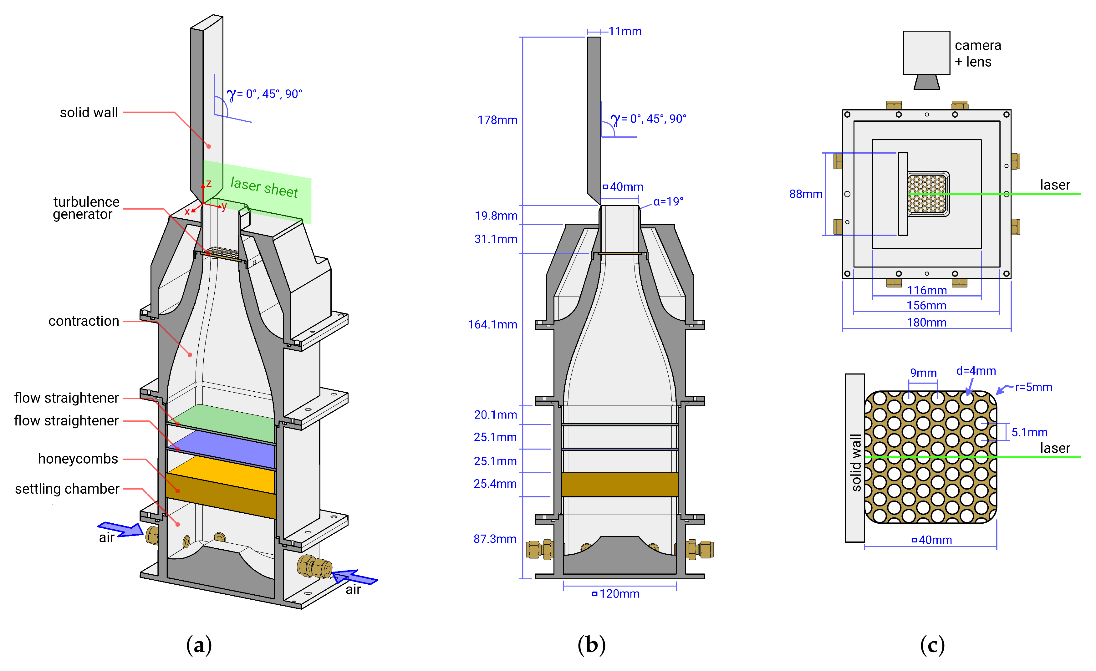
3.1. Experimental Setup
3.2. Numerical Setup
3.3. Summary of the Case Studies
4. Experimental Results
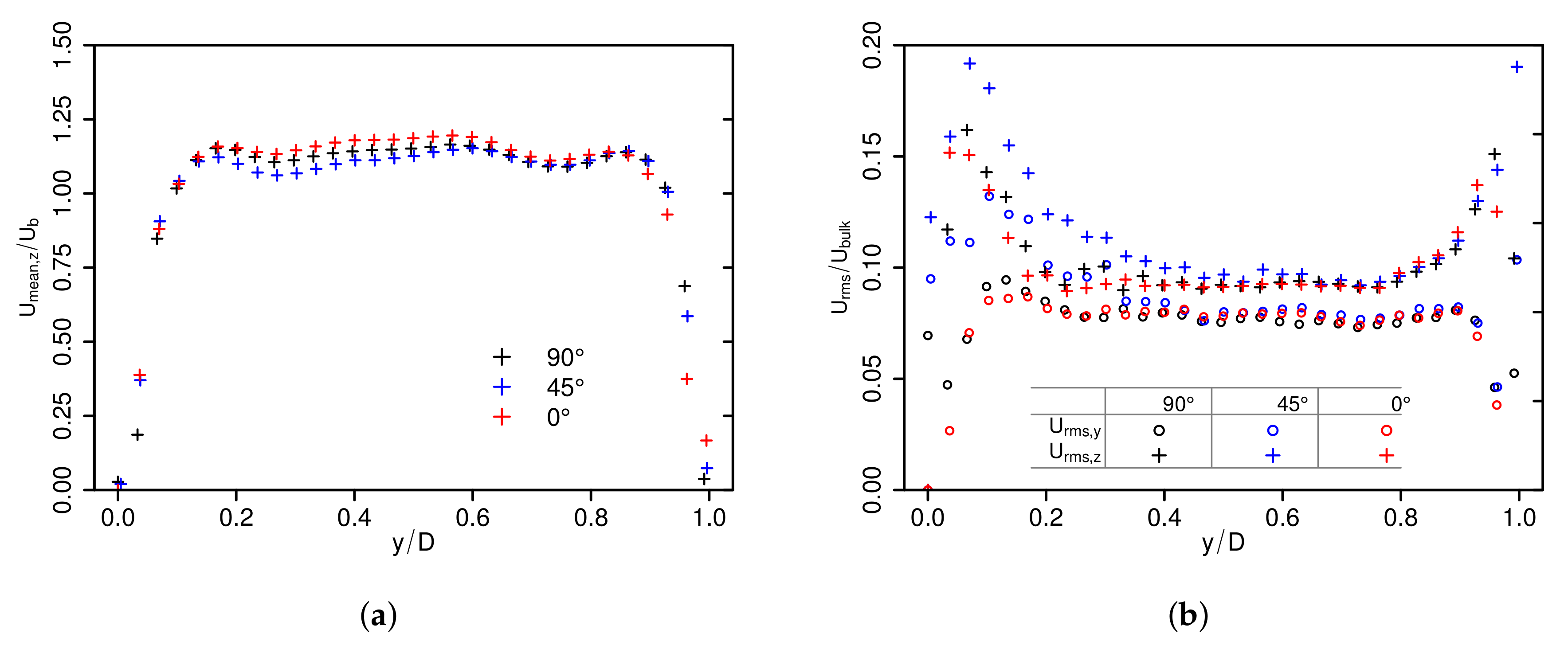
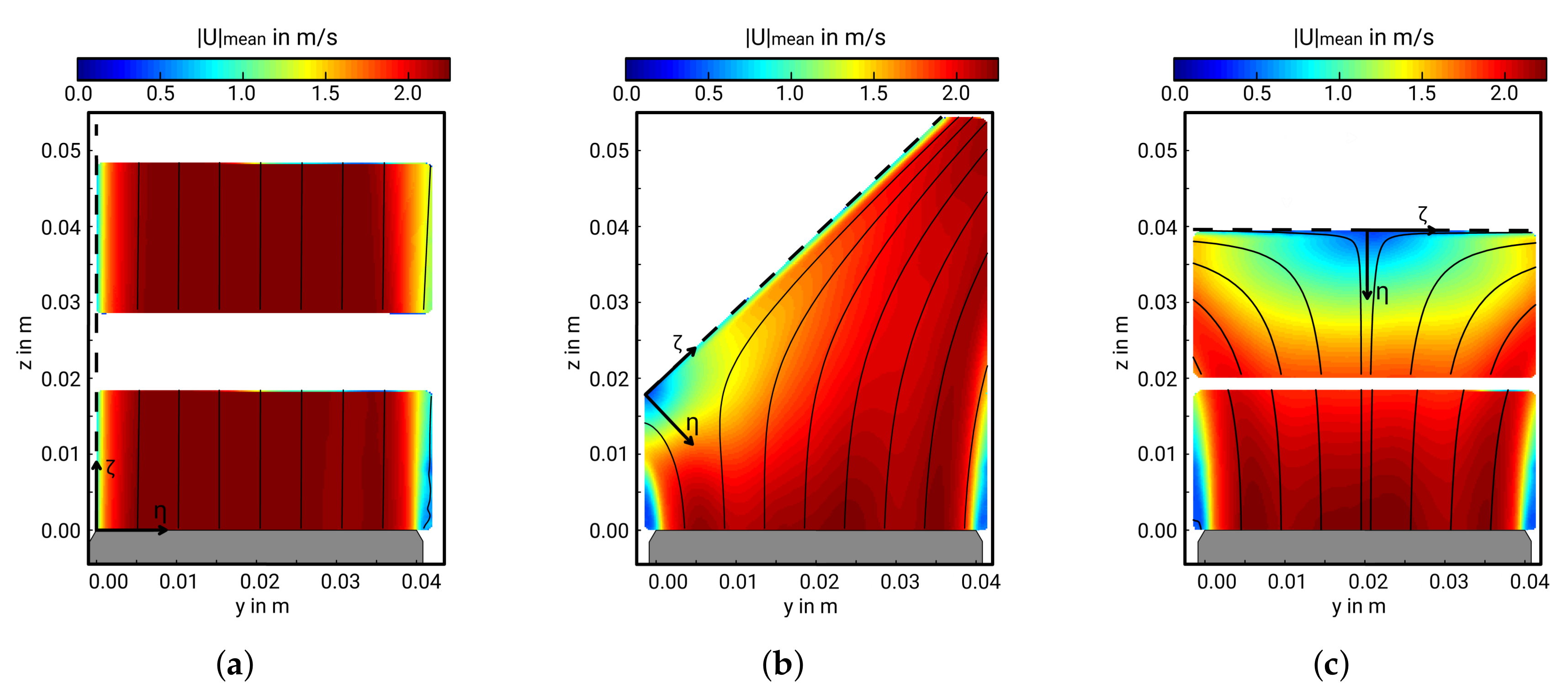
4.1. Mean Flow Properties
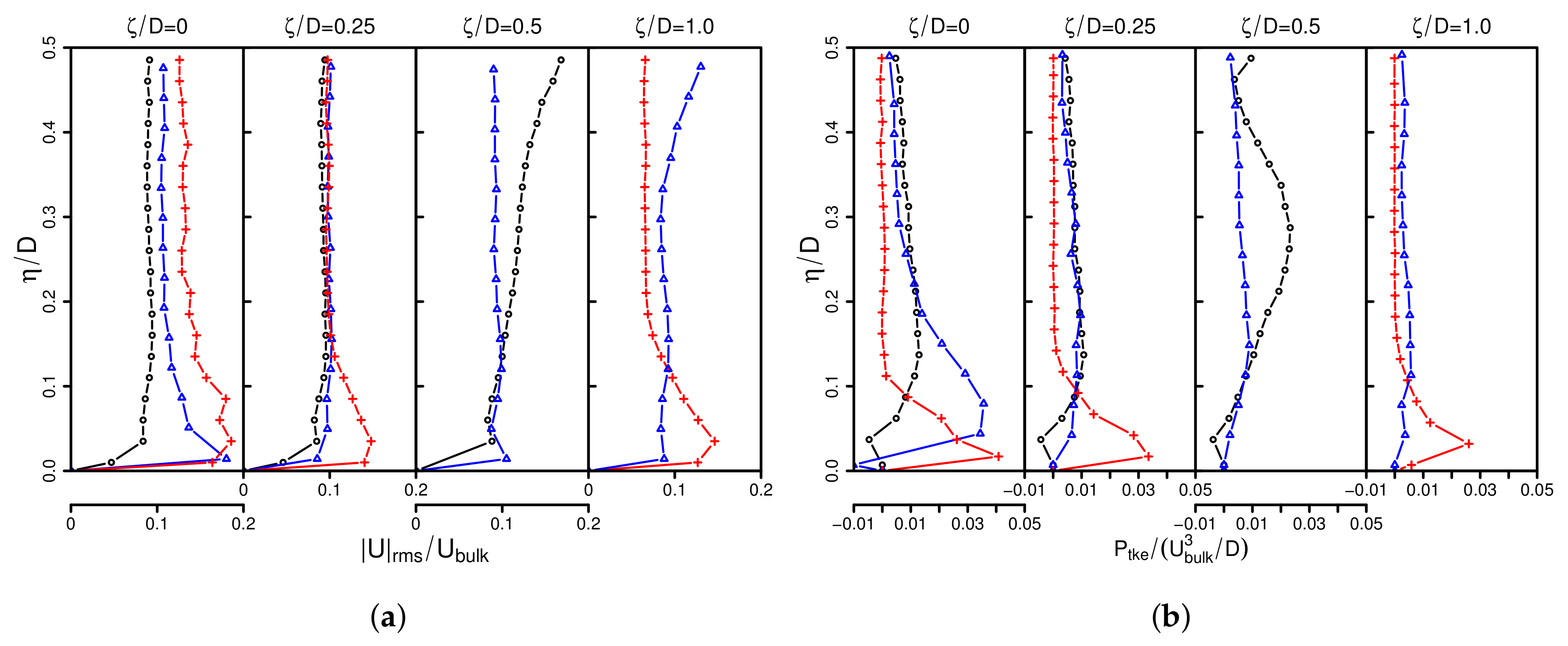
4.2. Turbulence Dynamics
5. Numerical Results
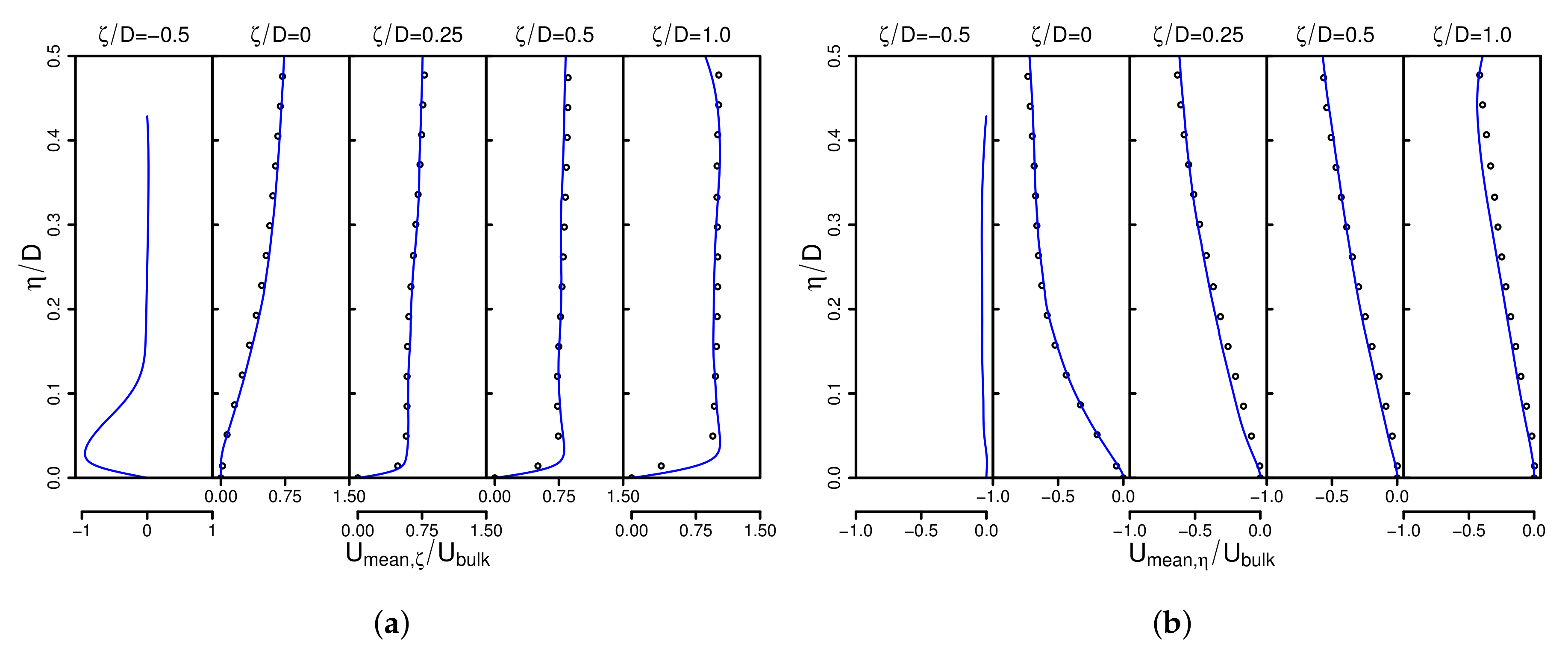
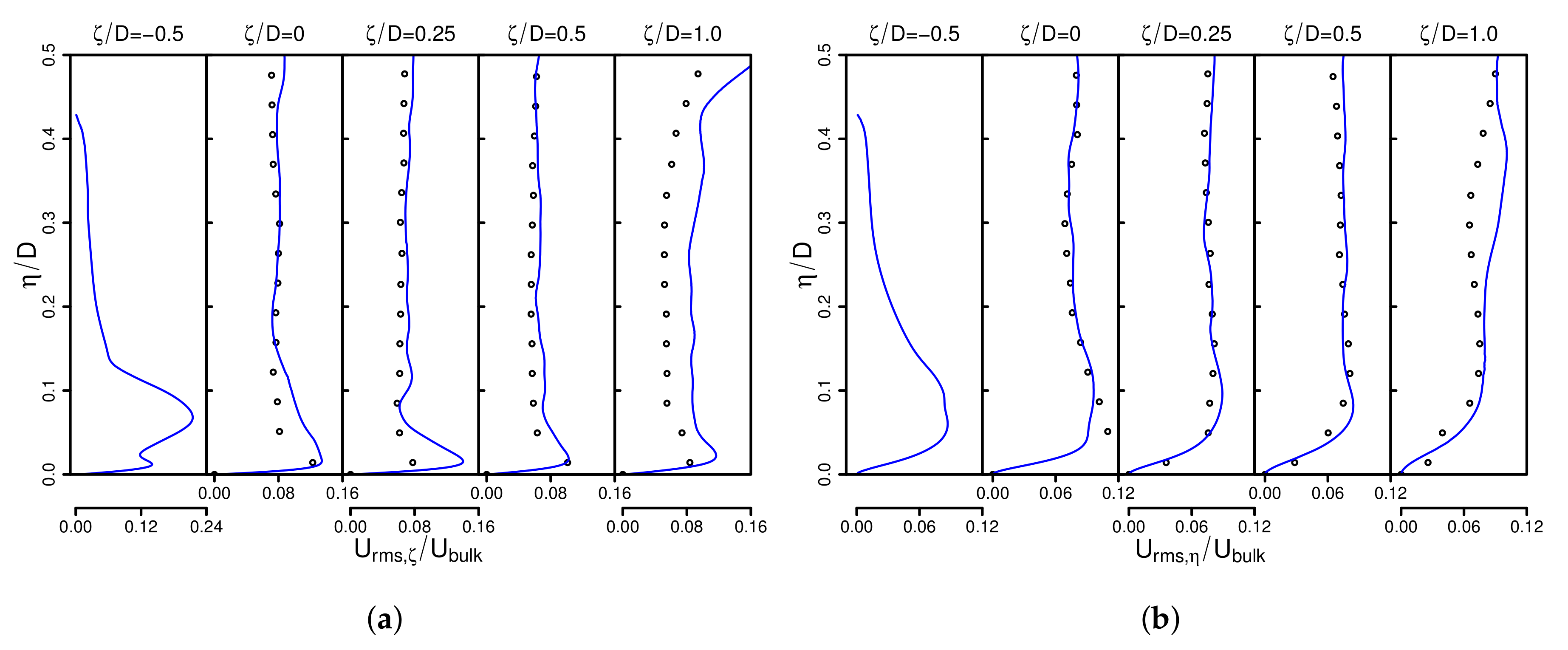
5.1. Comparison with Experimental Results
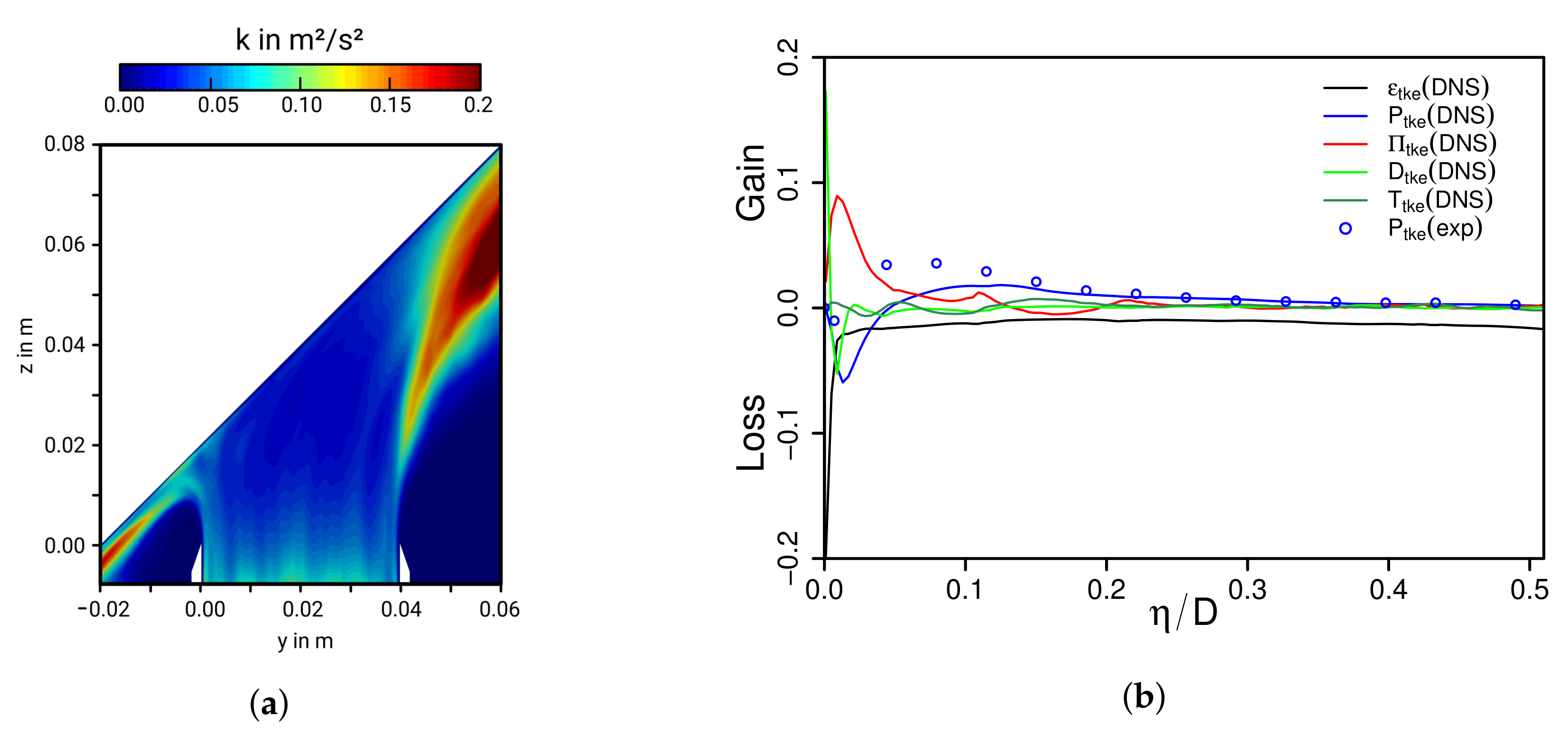
5.2. Budget of Turbulent Kinetic Energy Transport
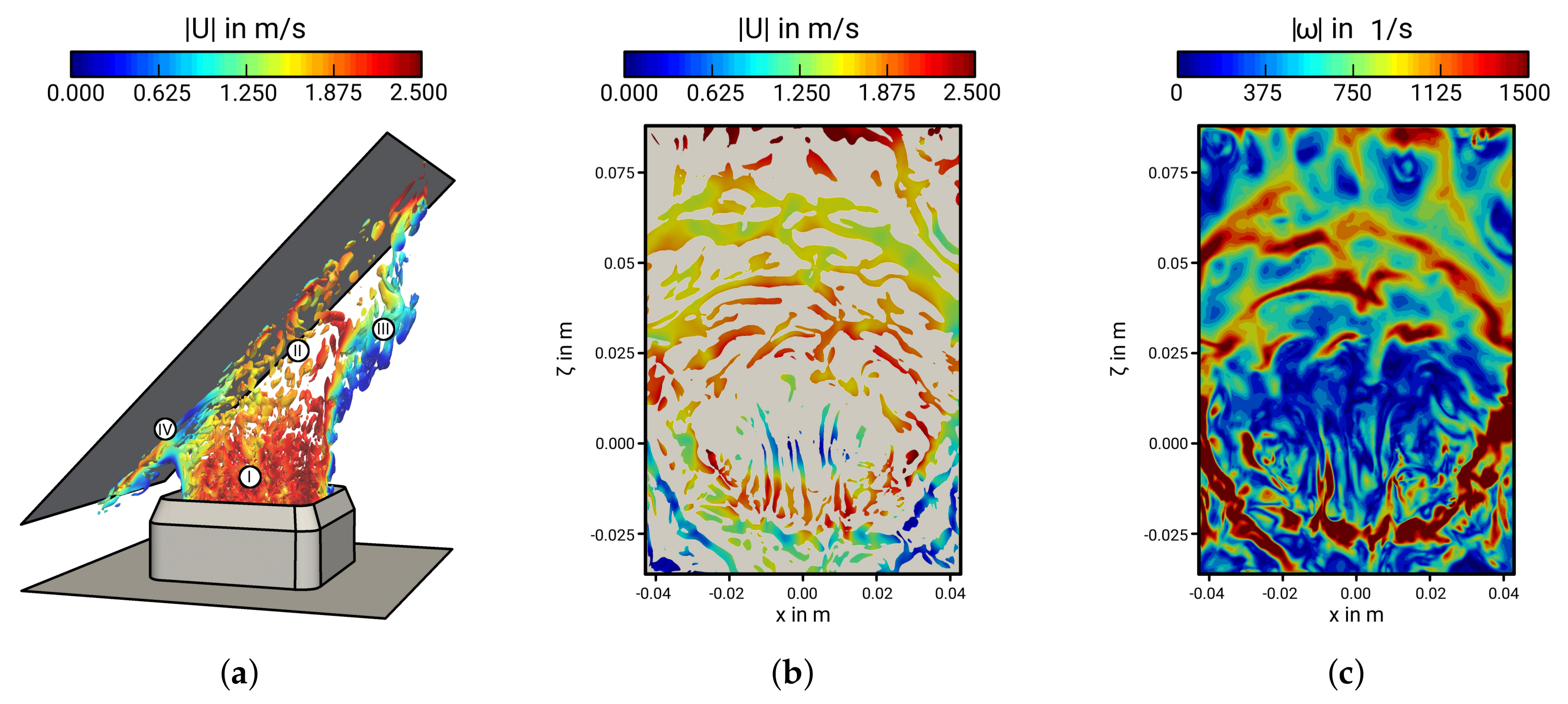
5.3. Turbulence Structures
5.4. Near-Wall Shear Stress
6. Concluding Remarks
- I
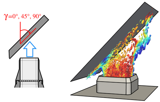
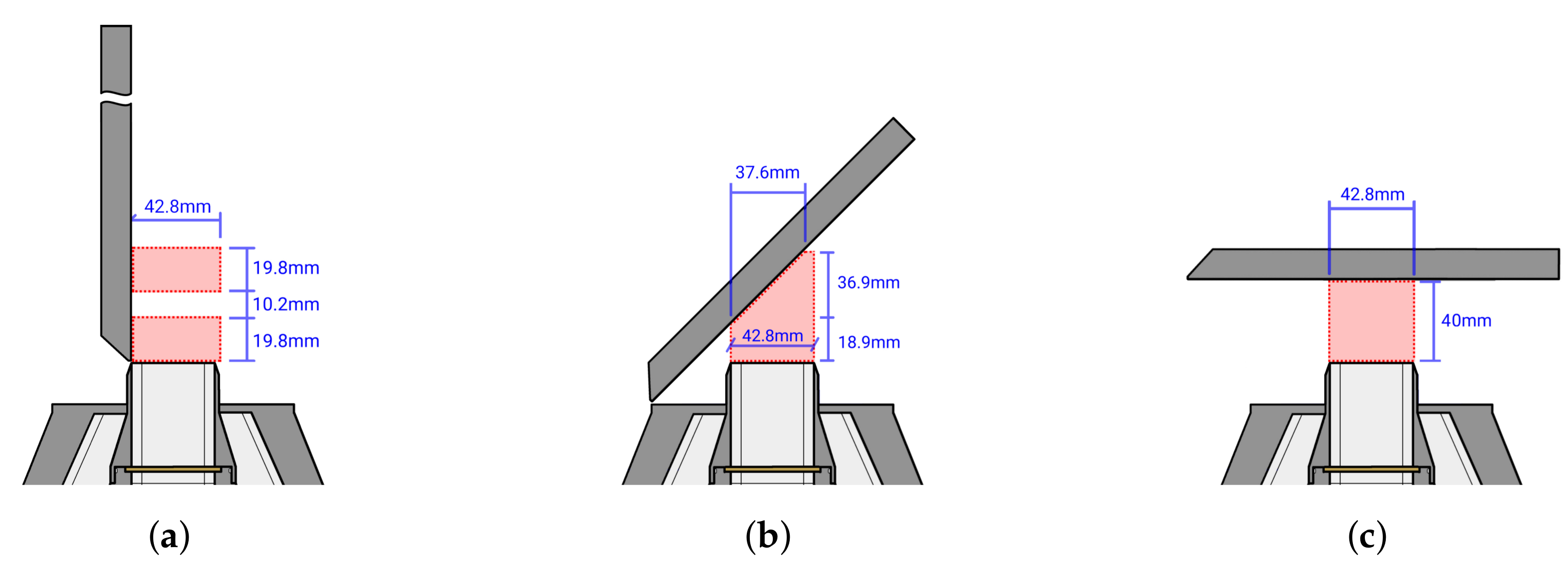
- Mean flow patterns are inherently different in the , and jet configurations. In particular, the -configuration resembles a boundary layer flow, while the stagnation region and wall-jets are predominant in the -configuration. Flow features of both configurations, namely boundary layer flow properties, stagnation point and strong wall/jet interactions, prevail in the -inclination case, which represents therefore a good generic benchmark test case for a wide range of technical applications.
- II
- It turns out that the production of turbulent kinetic energy appears negative at the stagnation region in the - and -configurations, which is balanced predominantly by pressure-related diffusion. In the case of the -inclination angle, the production term is always positive.
- III
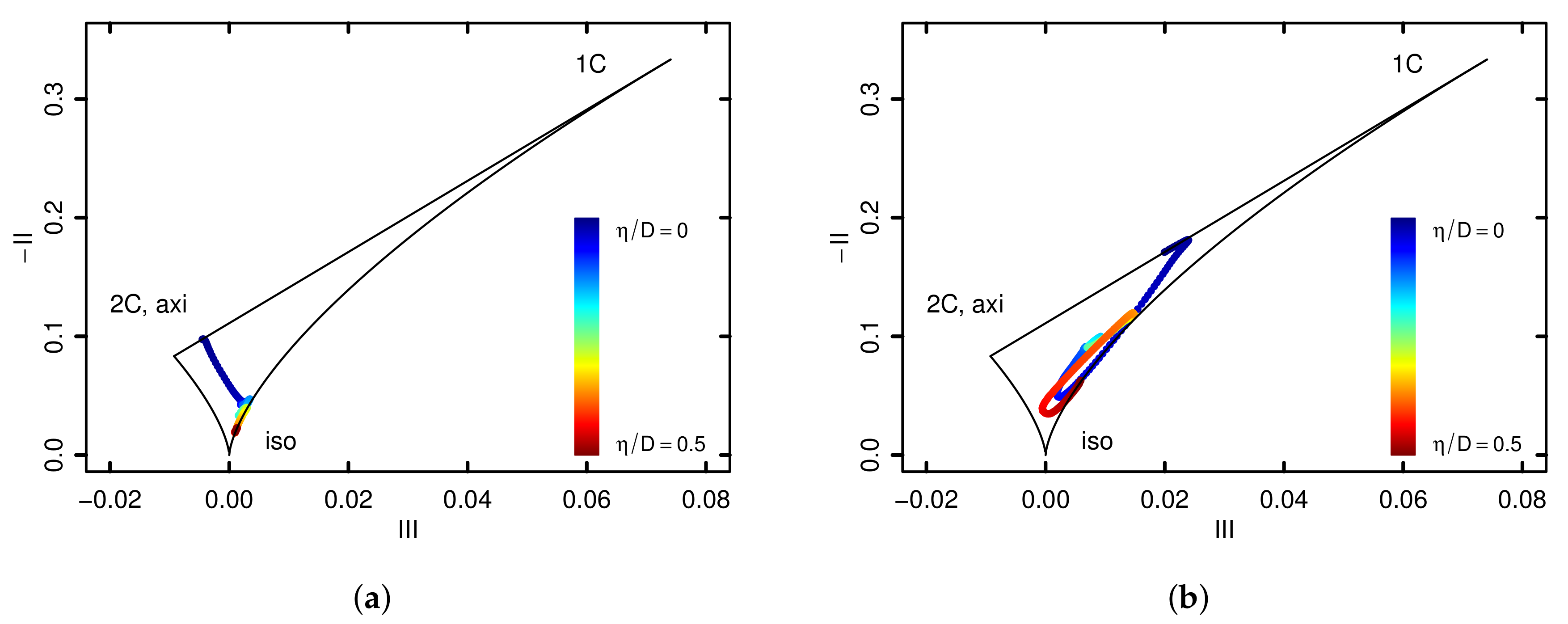
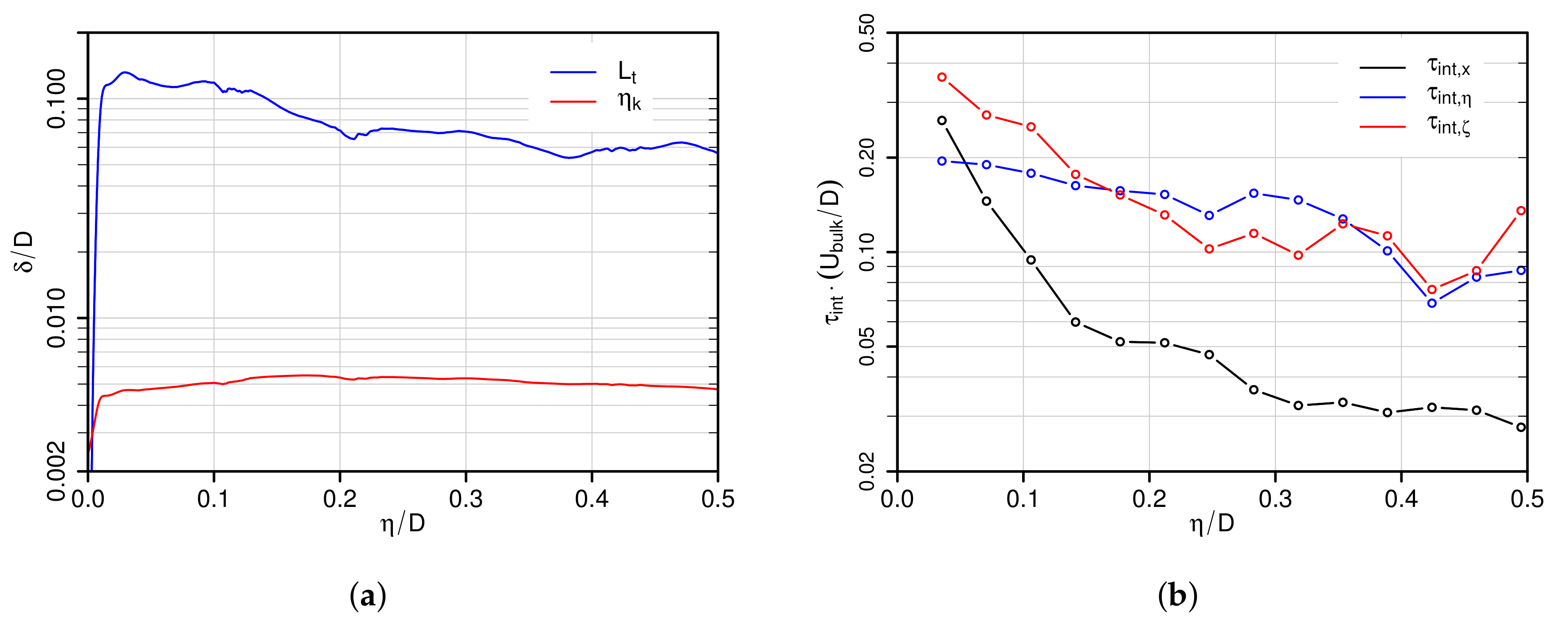
- By examining turbulent flow structures in the -configuration, it turns out that quasi-coherent thin streaks appear around the stagnation point. Thereby, the turbulence is essentially axisymmetric with large characteristic turbulence time scales. Further downstream, at the wall-jet region, the organization of the flow is predominantly toroidal, and the turbulence behaves similarly to that found in turbulent boundary layer flows.
- IV
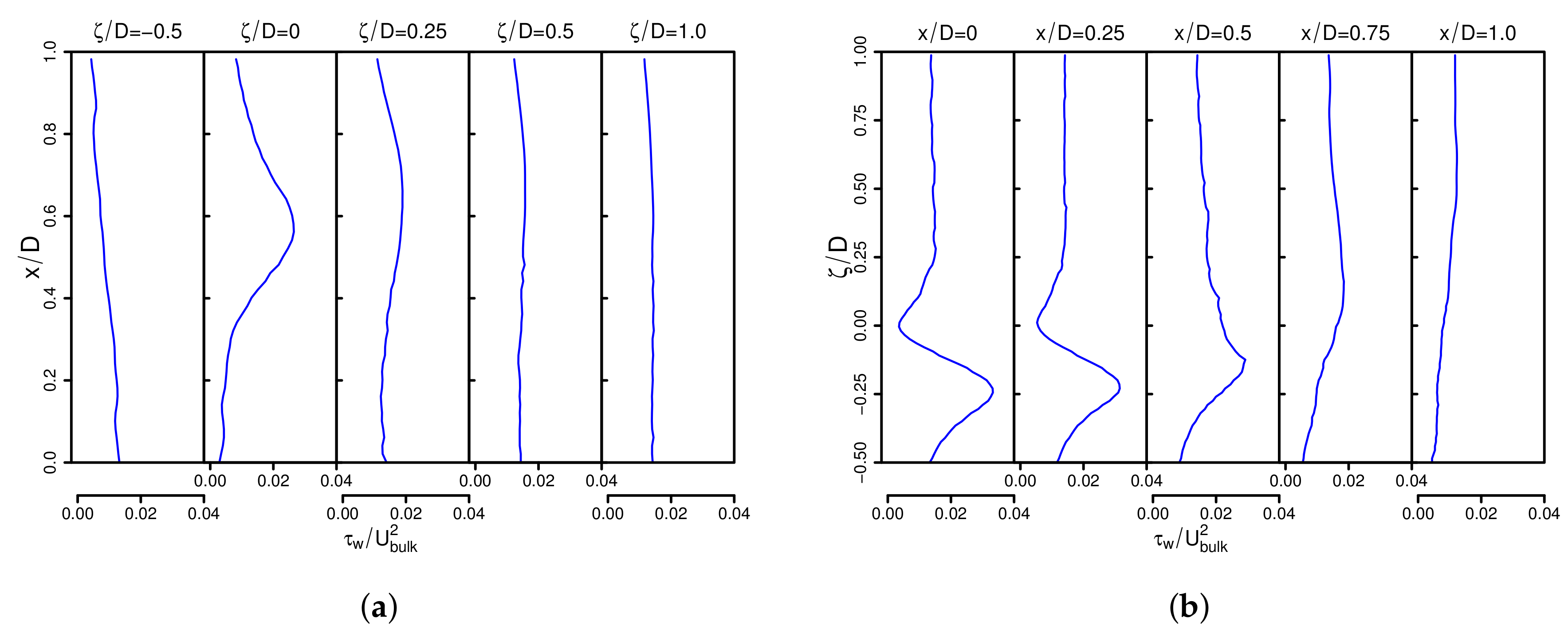
- In the case of the -inclination angle, near-wall shear stresses are very low at the stagnation point and primarily concentrated at the secondary opposed wall jet region. This suggests that the wall/flow interaction process depends inherently on the impinging angle and is obviously more intense in regions where the direction of the flow changes suddenly and the fluid is subject to high acceleration in the wall-parallel direction.
Acknowledgments
Author Contributions
Conflicts of Interest
Appendix A. Code Verification
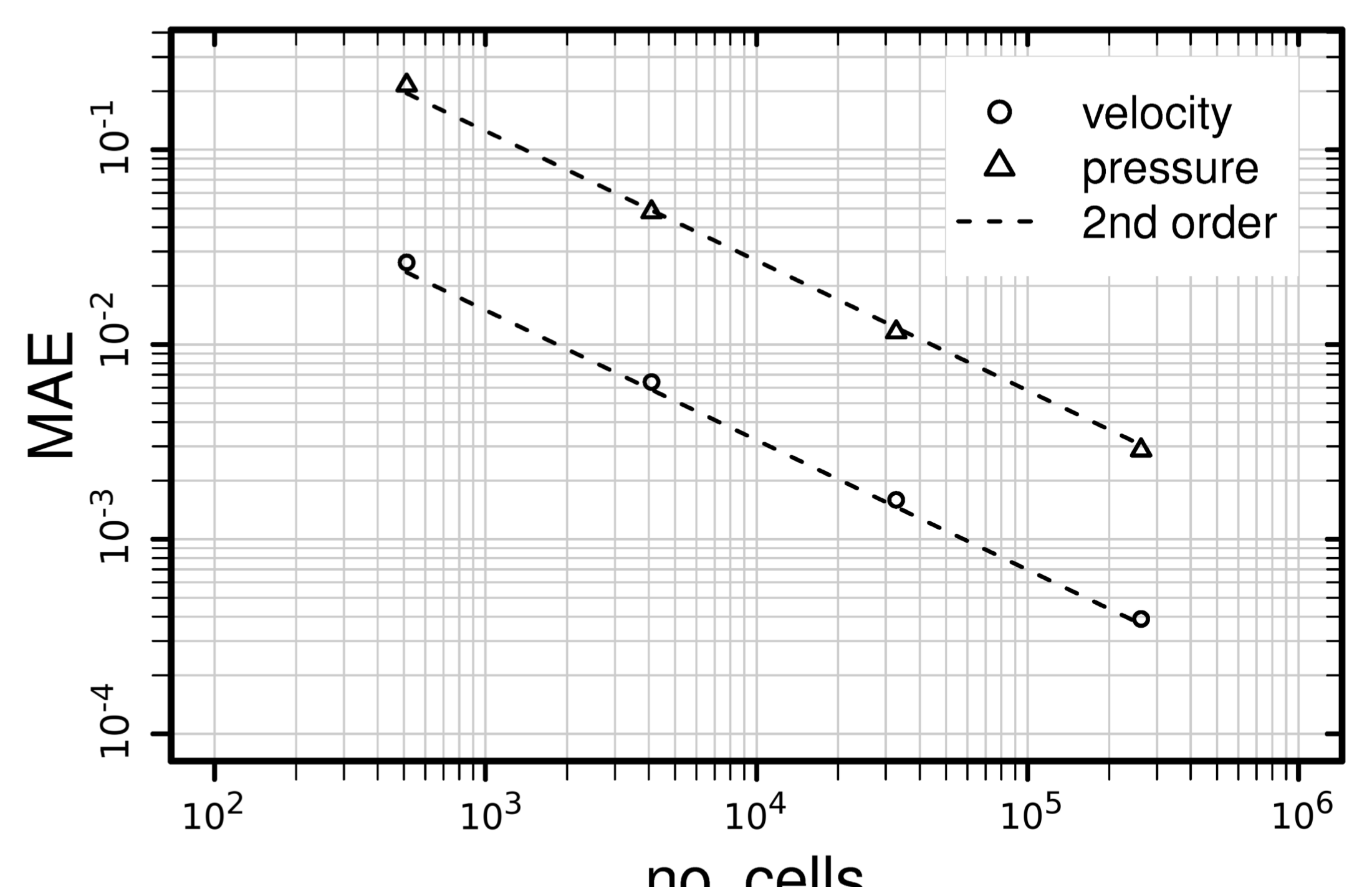
Appendix A.1. Spatial Accuracy
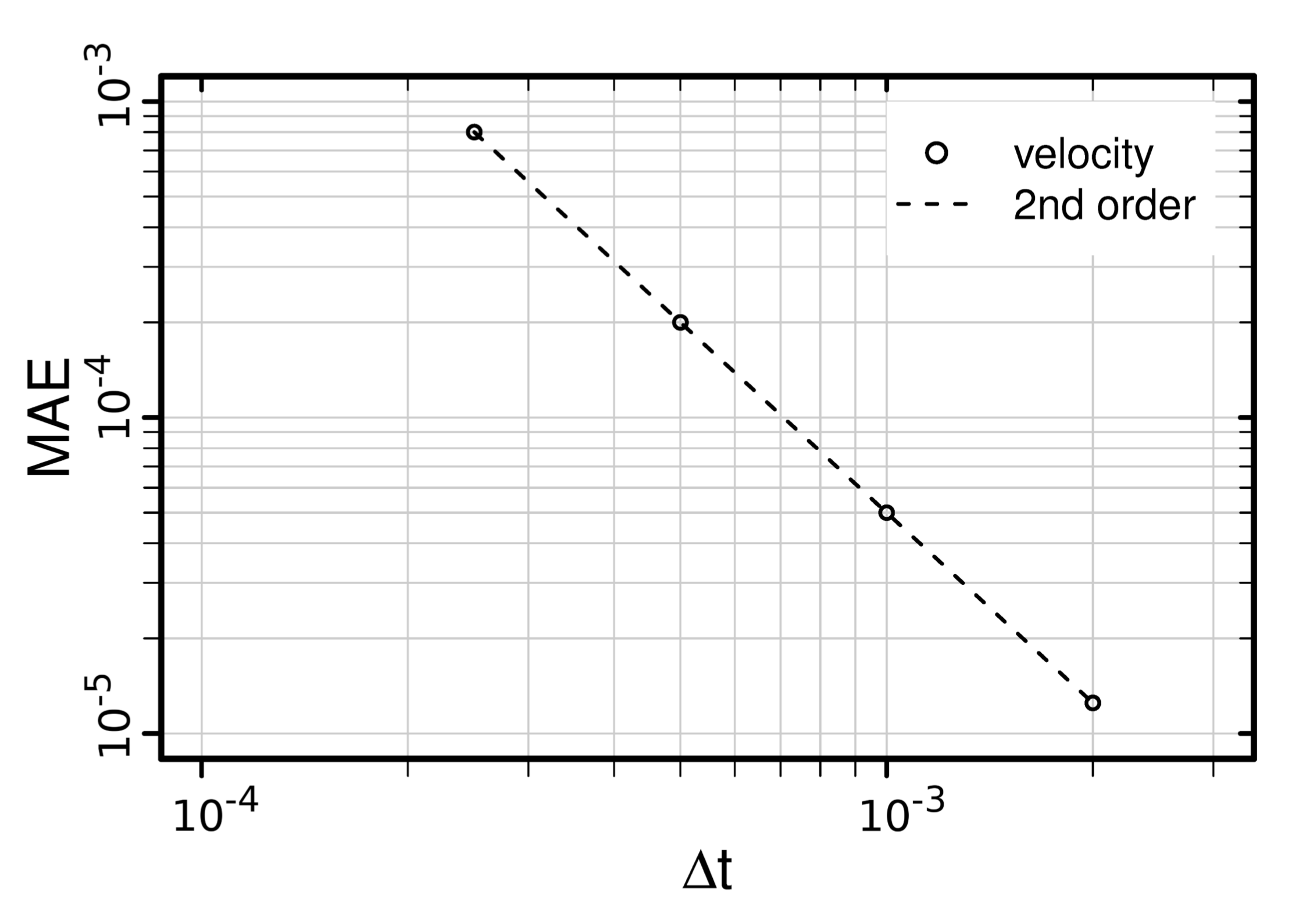
Appendix A.2. Temporal Accuracy
Appendix B. Inflow Conditions for Numerical Simulations
References
- Martin, H. Heat and mass transfer between impinging gas jets and solid surfaces. Adv. Heat Transf. 1997, 13, 1–60. [Google Scholar] [CrossRef]
- Jambunathan, K.; Lai, E.; Moss, M.A.; Button, B.L. A review of heat transfer data for single circular jet impingement. Int. J. Heat Fluid Flow 1992, 13, 106–115. [Google Scholar] [CrossRef]
- Viskanta, R. Heat transfer to impinging isothermal gas and flame jets. Exp. Therm. Fluid Sci. 1993, 6, 106–115. [Google Scholar] [CrossRef]
- Zuckerman, N.; Lior, N. Jet impingement heat transfer: Physics, correlations, and numerical modeling. Adv. Heat Transf. 2006, 39, 565–631. [Google Scholar] [CrossRef]
- Tummers, M.J.; Jacobse, J.; Voorbrood, S.G.J. Turbulent flow in the near field of a round impinging jet. Int. J. Heat Mass Transf. 2011, 54, 4939–4948. [Google Scholar] [CrossRef]
- Boughn, J.W.; Shimizu, S. Heat transfer measurements from a surface with uniform heat flux and an impinging jet. J. Heat Transf. 1989, 111, 1096–1098. [Google Scholar] [CrossRef]
- Cooper, D.; Jackson, D.C.; Launder, B.E.; Liao, G.X. Impinging jet studies for turbulence model assessment-I. Flow-field experiments. Int. J. Heat Mass Transf. 1993, 36, 2675–2684. [Google Scholar] [CrossRef]
- Nishino, K.; Samada, M.; Kasuya, K.; Torii, K. Turbulence statistics in the stagnation region of an axisymmetric impinging jet flow. Int. J. Heat Fluid Flow 1996, 17, 193–201. [Google Scholar] [CrossRef]
- Behrouzi, P.; McGuirk, J.J. Laser Doppler velocimetry measurements of twin-jet impingement flow for validation of computational models. Opt. Laser Eng. 1998, 30, 265–277. [Google Scholar] [CrossRef]
- Fairweather, M.; Hargrave, G. Experimental investigation of an axisymmetric, impinging turbulent jet. 1. Velocity field. Exp. Fluids 2002, 33, 464–471. [Google Scholar] [CrossRef]
- Geers, L.F.G.; Tummers, M.J.; Hanjalić, K. Experimental investigation of impinging jet arrays. Exp. Fluids 2004, 36, 946–958. [Google Scholar] [CrossRef]
- Katti, V.; Prabhu, S.V. Experimental study and theoretical analysis of local heat transfer distribution between smooth flat surface and impinging air jet from a circular straight pipe nozzle. Int. J. Heat Mass Transf. 2008, 51, 4480–4495. [Google Scholar] [CrossRef]
- Satake, S.; Kunugi, T. Direct numerical simulation of an impinging jet into parallel disks. Int. J. Numer. Methods Heat Fluid Flow 1998, 8, 768–780. [Google Scholar] [CrossRef]
- Chung, Y.M.; Luo, K.H. Unsteady Heat Transfer Analysis of an Impinging Jet. J. Heat Transf. 2002, 124, 1039–1048. [Google Scholar] [CrossRef]
- Hattori, H.; Nagano, Y. Direct numerical simulation of turbulent heat transfer in plane impinging jet. Int. J. Heat Fluid Flow 2004, 25, 749–758. [Google Scholar] [CrossRef]
- Wilke, R.; Sesterhenn, J. Numerical Simulation of Impinging Jets. In High Performance Computing in Science and Engineering ’14; Springer: Cham, Switzerland, 2015; pp. 275–287. [Google Scholar]
- Jainski, C.; Lu, L.; Sick, V.; Dreizler, A. Laser imaging investigation of transient heat transfer processes in turbulent nitrogen jets impinging on a heated wall. Int. J. Heat Mass Transf. 2014, 74, 101–112. [Google Scholar] [CrossRef]
- Behnia, M.; Parneix, S.; Durbin, P.A. Prediction of heat transfer in an axisymmetric turbulent jet impinging on a flat plate. Int. J. Heat Mass Transf. 1998, 41, 1845–1855. [Google Scholar] [CrossRef]
- Hanjalić, K.; Popovac, M.; Hadžiabdić, M. A robust near-wall elliptic-relaxation eddy-viscosity turbulence model for CFD. Int. J. Heat Fluid Flow 2004, 25, 1047–1051. [Google Scholar] [CrossRef]
- Jaramillo, J.E.; Pérez-Segarra, C.D.; Rodriguez, I.; Oliva, A. Numerical study of plane and round impinging jets using RANS models. Numer. Heat Transf. B Fundam. 2008, 54, 213–237. [Google Scholar] [CrossRef]
- Hadžiabdić, M.; Hanjalić, K. Vortical structures and heat transfer in a round impinging jet. J. Fluid Mech. 2008, 596, 221–260. [Google Scholar] [CrossRef]
- Uddin, N.; Neumann, A.O.; Weigand, B. LES simulations of an impinging jet: On the origin of the second peak in the Nusselt number distribution. Int. J. Heat Mass Transf. 2013, 57, 356–368. [Google Scholar] [CrossRef]
- Krumbein, B.; Jakirlić, S.; Tropea, C. VLES study of a jet impinging onto a heated wall. Int. J. Heat Fluid Flow 2017, in press. [Google Scholar] [CrossRef]
- Hall, J.W.; Ewing, D. On the dynamics of the large-scale structures in round impinging jets. J. Fluid Mech. 2005, 555, 439–458. [Google Scholar] [CrossRef]
- Hall, J.W.; Ewing, D. The development of the large-scale structures in round impinging jets exiting long pipes at two Reynolds numbers. Exp. Fluids 2005, 38, 50–58. [Google Scholar] [CrossRef]
- Lee, J.; Lee, S.-J. Stagnation region heat transfer of a turbulent axisymmetric jet impingement. Exp. Heat Transf. 1999, 12, 137–156. [Google Scholar] [CrossRef]
- Dairay, T.; Fortuné, V.; Lamballais, E.; Brizzi, L.-E. Direct numerical simulation of a turbulent jet impinging on a heated wall. J. Fluid Mech. 2015, 764, 362–394. [Google Scholar] [CrossRef]
- Wilke, R.; Sesterhenn, J. Statistics of fully turbulent impinging jets. J. Fluid Mech. 2017, 825, 795–824. [Google Scholar] [CrossRef]
- Schmitt, M.; Frouzakis, C.E.; Tomboulides, A. Direct numerical simulation of multiple cycles in a valve/piston assembly. Phys. Fluids 2014, 26, 035105. [Google Scholar] [CrossRef]
- Yang, Q.; Zhang, Z.; Liu, M.; Hu, J.A. Numerical Simulation of Fluid Flow inside the Valve. Procedia Eng. 2011, 23, 543–550. [Google Scholar] [CrossRef]
- Chorin, A.J. Numerical Solution of the Navier-Stokes Equations. Math. Comput. 1968, 22, 745–762. [Google Scholar] [CrossRef]
- Issa, R.I. Solution of the implicitly discretised fluid flow equations by operator-splitting. J. Comput. Phys. 1986, 62, 40–65. [Google Scholar] [CrossRef]
- Patankar, S.V.; Spalding, D.B. A calculation procedure for heat, mass and momentum transfer in three-dimensional parabolic flows. Int. J. Heat Mass Transf. 1972, 15, 1787–1806. [Google Scholar] [CrossRef]
- Vuorinen, V.; Keskinen, J.-P.; Duwig, C.; Boersma, B.J. On the implementation of low-dissipative Runge–Kutta projection methods for time dependent flows using OpenFOAM. Comput. Fluids 2014, 93, 153–163. [Google Scholar] [CrossRef]
- Van der Houwen, P.J. Explicit Runge-Kutta formulas with increased stability boundaries. Numer. Math. 1972, 20, 149–164. [Google Scholar] [CrossRef]
- Hirsch, C. Numerical Computation of Internal and External Flows: The Fundamentals of Computational Fluid Dynamics, 2nd ed.; Butterworth-Heinemann: Oxford, UK, 2007; ISBN 9780080550022. [Google Scholar]
- González Hernandéz, M.A.; Moreno López, A.I.; Jarzabek, A.A.; Perales Perales, J.M.; Wu, Y.; Xiaoxiao, S. Design Methodology for a Quick and Low-Cost Wind Tunnel, Wind Tunnel Designs and Their Diverse Engineering Applications; InTechOpen: London, UK, 2013. [Google Scholar] [CrossRef]
- Grötzbach, G. Spatial resolution requirements for direct numerical simulation of the Rayleigh-Bérnard convection. J. Comput. Phys. 1983, 49, 241–264. [Google Scholar] [CrossRef]
- Nicoud, F.; Ducros, F. Subgrid-scale stress modelling based on the square of the velocity gradient tensor. Flow Turbul. Combust. 1999, 62, 183–200. [Google Scholar] [CrossRef]
- Spalding, D.B. A Single formula for the “Law of the Wall”. J. Appl. Mech. 1961, 28, 455–458. [Google Scholar] [CrossRef]
- Pope, S.B. Turbulent Flows; 11th Printing; Cambridge University Press: Cambridge, UK, 2011; ISBN 9780521598866. [Google Scholar]
- Hunt, J.C.R.; Wray, A.A.; Moin, P. Eddies, stream, and convergence zones in turbulent flows. In Proceedings of the 1988 Summer Program, Stanford University, CA, USA, June 1988; pp. 193–208. [Google Scholar]
- Launder, B.E. Numerical computation of convective heat transfer in complex turbulent flows: Time to abandon wall functions? Int. J. Heat Mass Transf. 1984, 27, 1485–1491. [Google Scholar] [CrossRef]
- Launder, B.E. On the computation of convective heat transfer in complex turbulent flows. J. Heat Transf. 1988, 110, 1112–1128. [Google Scholar] [CrossRef]
- Shih, T.-H.; Povinelli, L.A.; Liu, N.-S. Application of generalized wall function for complex turbulent flows. J. Turbul. 2003, 4, N15. [Google Scholar] [CrossRef]
- Craft, T.J.; Gerasimov, A.V.; Iacovides, H.; Launder, B.E. Progress in the generalization of wall-function treatments. Int. J. Heat Fluid Flow 2002, 23, 148–160. [Google Scholar] [CrossRef]
- Suga, K.; Craft, T.J.; Iacovides, H. An analytical wall-function for turbulent flows and heat transfer over rough walls. Int. J. Heat Fluid Flow 2006, 27, 852–866. [Google Scholar] [CrossRef]
- Craft, T.J.; Gant, S.E.; Iacovides, H.; Launder, B.E. A new wall function strategy for complex turbulent flows. Numer. Heat Transf. B Fundam. 2004, 45, 301–318. [Google Scholar] [CrossRef]
- El Hassan, M.; Assoum, H.H.; Sobolik, V.; Vétel, J.; Abed-Meraim, K.; Garon, A.; Sakout, A. Experimental investigation of the wall shear stress and the vortex dynamics in a circular impinging jet. Exp. Fluids 2012, 52, 1475–1489. [Google Scholar] [CrossRef]
- Tu, C.V.; Wood, D.H. Wall pressure and shear stress measurements beneath an impinging jet. Exp. Therm. Fluid Sci. 1996, 13, 364–373. [Google Scholar] [CrossRef]
- Salari, K.; Knupp, P. Code Verification by the Method of Manufactured Solutions; SAND2000-1444; SciTech Connect: Washington, DC, USA, 2000. [Google Scholar]
- Shunn, L.; Ham, F. Method of Manufactured Solutions Applied to Variable-Density Flow Solvers. In Annual Research Briefs; Center for Turbulence Research: Stanford, CA, USA, 2007; pp. 155–168. [Google Scholar]
- Roache, P.J. Verification and Validation in Computational Science and Engineering, 1nd ed.; Hermosa Publishers: Socorro, NM, USA, 1998; ISBN 9780913478080. [Google Scholar]
- Oberkampf, W.L.; Roy, C.J. Verification and Validation in Scientific Computing; Cambridge University Press: Cambridge, UK, 2010; ISBN 978-0-521-11360-1. [Google Scholar]
- Taylor, G.I.; Green, A.E. Mechanism of the production of small eddies from large ones. Proc. R. Soc. A Math. Phys. 1937, 151, 499–521. [Google Scholar] [CrossRef]
- Joung, Y.; Choi, S.-U.; Choi, J.I. Direct numerical simulation of turbulent flow in a square duct: Analysis of secondary flows. J. Eng. Mech. ASCE 2007, 133, 213–221. [Google Scholar] [CrossRef]
- Gavrilakis, S. Numerical simulation of low-Reynolds-number turbulent flow through a straight square duct. J. Fluid Mech. 1992, 244, 101–129. [Google Scholar] [CrossRef]


| Configuration | Experiment | DNS |
|---|---|---|
| -inclination |
| |
| -inclination |
|
|
| -inclination |
|
© 2018 by the authors. Licensee MDPI, Basel, Switzerland. This article is an open access article distributed under the terms and conditions of the Creative Commons Attribution (CC BY) license (http://creativecommons.org/licenses/by/4.0/).
Share and Cite
Ries, F.; Li, Y.; Rißmann, M.; Klingenberg, D.; Nishad, K.; Böhm, B.; Dreizler, A.; Janicka, J.; Sadiki, A. Database of Near-Wall Turbulent Flow Properties of a Jet Impinging on a Solid Surface under Different Inclination Angles. Fluids 2018, 3, 5. https://doi.org/10.3390/fluids3010005
Ries F, Li Y, Rißmann M, Klingenberg D, Nishad K, Böhm B, Dreizler A, Janicka J, Sadiki A. Database of Near-Wall Turbulent Flow Properties of a Jet Impinging on a Solid Surface under Different Inclination Angles. Fluids. 2018; 3(1):5. https://doi.org/10.3390/fluids3010005
Chicago/Turabian StyleRies, Florian, Yongxiang Li, Martin Rißmann, Dario Klingenberg, Kaushal Nishad, Benjamin Böhm, Andreas Dreizler, Johannes Janicka, and Amsini Sadiki. 2018. "Database of Near-Wall Turbulent Flow Properties of a Jet Impinging on a Solid Surface under Different Inclination Angles" Fluids 3, no. 1: 5. https://doi.org/10.3390/fluids3010005
APA StyleRies, F., Li, Y., Rißmann, M., Klingenberg, D., Nishad, K., Böhm, B., Dreizler, A., Janicka, J., & Sadiki, A. (2018). Database of Near-Wall Turbulent Flow Properties of a Jet Impinging on a Solid Surface under Different Inclination Angles. Fluids, 3(1), 5. https://doi.org/10.3390/fluids3010005