One Dimensional Model for Droplet Ejection Process in Inkjet Devices

Mechanical Engineering, School of Engineering and Computer Science, Washington State University—Vancouver, 14204 NE Salmon Creek Ave., Vancouver, WA 98686, USA
*
Author to whom correspondence should be addressed.
Fluids 2018, 3(2), 28; https://doi.org/10.3390/fluids3020028
Submission received: 6 March 2018
/
Revised: 11 April 2018
/
Accepted: 18 April 2018
/
Published: 23 April 2018
(This article belongs to the Special Issue Reduced Order Modeling of Fluid Flows)
Abstract
:In recent years, physics-based computer models have been increasingly applied to design the drop-on-demand (DOD) inkjet devices. The initial design stage for these devices often requires a fast turnaround time of computer models, because it usually involves a massive screening of a large number of design parameters. Thus, in the present study, a 1D model is developed to achieve the fast prediction of droplet ejection process from DOD devices, including the droplet breakup and coalescence. A popular 1D slender-jet method (Egger, 1994) is adopted in this study. The fluid dynamics in the nozzle region is described by a 2D axisymmetric unsteady Poiseuille flow model. Droplet formation and nozzle fluid dynamics are coupled, and hence solved together, to simulate the inkjet droplet ejection. The arbitrary Lagrangian–Eulerian method is employed to solve the governing equations. Numerical methods have been proposed to handle the breakup and coalescence of droplets. The proposed methods are implemented in an in-house developed MATLAB code. A series of validation examples have been carried out to evaluate the accuracy and the robustness of the proposed 1D model. Finally, a case study of the inkjet droplet ejection with different Ohnesorge number (Oh) is presented to demonstrate the capability of the proposed 1D model for DOD inkjet process. Our study has shown that 1D model can significantly reduce the computational time (usually less than one minute) yet with acceptable accuracy, which makes it very useful to explore the large parameter space of inkjet devices in a short amount of time.
1. Introduction
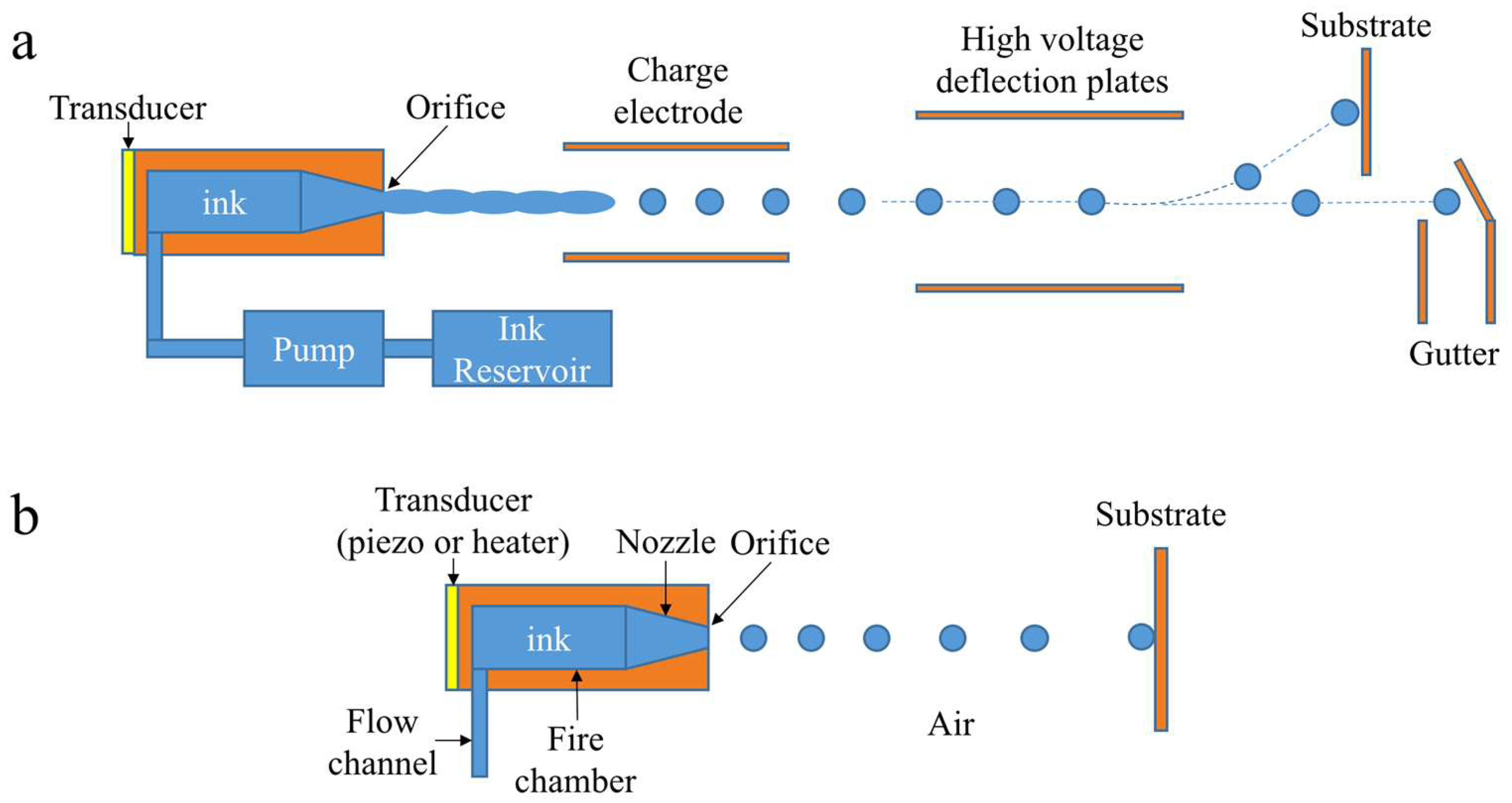
Inkjet technologies have advanced significantly since the first commercialization in 1970s, with focus in text and graphic printing. The dramatic expansion of printing material [1] makes it not only a term describing graphic printing, but also a term covering a range of technologies which involve the ejection of droplets from a printhead onto a substrate. Due to its ability to precisely deliver picoliter-scale volumes of liquid at high speed and low cost, inkjet technologies have already extended beyond the traditional printing area into a wide variety of emerging applications, such as additive manufacturing [2], electronic device prototyping [3], pharmaceutics [4], tissue engineering [5] and spray cooling of electronics [6]. Generally speaking, inkjet devices are classified as one of two kinds: continuous inkjet (CIJ) and drop-on-demand (DOD) inkjet, which are distinguished by the form of the ejected liquid. The schematic of these two systems are shown in Figure 1. A CIJ device ejects a continuous stream of liquid, whereas a DOD device ejects droplets at a regular time interval, and is controlled by electronic signals. Further, depending on the actuation of the driving pulse, there are two major varieties of DOD inkjets: piezoelectric inkjet (PIJ) and thermal inkjet (TIJ) [7]. For PIJ, the pressure gradient is generated by the deformation of a piezoelectric transducer (PZT). By contrast, TIJs use a thin film resistor to boil part of the ink, generating an expanding bubble that pushes ink out of the nozzle.
When the liquid is ejected from the DOD inkjet device, it undergoes a series of physical events: 1. the drop emerges from the nozzle due to actuation; 2. the drop pinches off from the nozzle; 3. the drop breaks up into main droplet followed by multiple satellite droplets; 4. the satellite droplets may coalesce or catch up to and recombine with the main droplet. Satellite droplets often cause detrimental effects on printing quality, because they tend to scatter on the substrate. Therefore, fundamental understanding of droplet ejection is crucial to various applications of the DOD inkjet technologies.
Due to the recent significant advances of high-speed imaging systems, modern experimental methods can reveal great details of inkjet droplet ejection process [8,9,10,11], and have become an indispensable step in the development of inkjet devices. However, it is not cost effective to use empirical methods to optimize inkjet devices because of the high cost, long development time, and complexity. As a result, physics-based computer simulations become increasingly popular in inkjet industry. A 2D axisymmetric simulation of droplet ejection in DOD inkjet is pioneered by Fromm [12], who used the marker-and-cell method-based vorticity-stream function to solve Navier–Stokes (NS) equations in axisymmetric condition. Currently, finite element (FE) method [13,14,15,16], volume-of-fluid (VOF) method [17,18,19,20,21,22] and level-set (LS) method [23,24,25] are the most common methods used to solve the multiphase flow problem in inkjet process. Both TIJ and PIJ have been successfully simulated by a number of researchers [18,21,22]. Non-Newtonian fluids printing, which are almost used in all non-printing applications of inkjet, were also simulated by Morrison and his colleagues [13,16,26]. More recently, Tan et al. [22,27] carried out high fidelity 3D simulations of TIJ printhead including vapor bubble growth/collapse and refill of firing chamber for an actual complex printhead. However, 2D and 3D methods are usually computationally expensive, and hence, are not suitable for a large-scale screening of design parameters in the early design stage, such as nozzle geometry, fluid properties, and operation conditions. In addition, it is noteworthy that commercial software packages, such as FLOW-3D [28,29], CFD-ACE+ [30] and COMSOL [31], are also frequently used in simulation of droplet ejection, but the license price and complexity of operation prevent them from being extensively used by developers of DOD inkjet devices.
Therefore, 1D simulation seems to be a reasonable choice for vast-selection of design parameters, due to its low demand on computing resources and rapid turnout time. Adams and Roy [32] first carried out a 1D simulation of droplet ejection in a DOD inkjet printhead. They added the viscous term into the inviscid-slice model proposed by Lee [33]. Their 1D equations were solved by the MacCormack’s predictor-corrector algorithm in Lagrangian coordinates, but the result shows distinct discrepancies from Fromm’s 2D axisymmetric simulation with the same driving pressure boundary condition [34]. For example, their droplets have earlier breakup time and higher final velocity than 2D model. Shield and Bogy [35] presented a different method based on Green’s Cosserat theory [36]. They employed the MacCormack’s algorithm in an Eulerian grid to solve the governing equations. By including and excluding the radial inertial term of the 1D Cosserat equations for an inviscid axisymmetric jet, they found that, at a higher Weber number, the omission of radial inertia has a greater effect on the droplet profiles than at a lower Weber number. Wallace [37] simulated the performance of a PIJ device based on a method of characteristics solution to the hydraulic transients in the devices. With inclusion of PZT dynamics in his model, he studied the effect of voltage waveform on droplet formation, which matched experiments qualitatively. These published studies have demonstrated the significant advantage of 1D models over 2D or 3D models in terms of the computational cost. For example, even with the very low computing capacity (38 MHz CPU) in 1980s, it takes only about 30 s for Shield [35] to complete a droplet calculation until breakup. From the mid-90s, a 1D lubrication approximation of NS equations proposed by Eggers and DuPont [38] (E&D) has gained an extensive popularity in investigation of fluid dynamics of microscopic droplets (thin liquid filaments). Compared with Lee’s and Green’s theories, its success lies in its self-consistent property, and the inclusion of radial inertial and viscous force. This model has been validated in various areas (e.g., dripping [39,40], continuous jetting [41,42,43], and filament contraction [10,44,45]), by theories, experiments, and full 3D simulations. To our best knowledge, so far, only Shin et al. [46] has applied E&D model to DOD inkjet with a focus on the mass transport rate of a squeeze mode PIJ. However, there is no droplet ejection process reported in their study. Through our literature survey, we find that a comprehensive and rigorous validation of 1D models for droplet ejection (e.g., droplet shape, velocity, volume, and breakup time) in inkjet technologies is still missing in these published studies. As a result, it remains unclear how well the 1D models predict the inkjet process.
The objective of this paper is to investigate whether 1D simulations can be applied to DOD inkjet droplet ejection through a comprehensive validation. As the first stage of a long term study, we only considered Newtonian fluid in this work. Fluid physical events, including the droplet formation, droplet breakup, droplet coalescence, and meniscus motion at the orifice are included into our 1D model. The droplet emergence from the orifice is based on the E&D’s 1D equations of motion which are solved by method of lines (MOL) in a moving uniform staggered mesh. The shape-preserving piecewise cubic interpolation and third-order polynomial curve are employed to treat the coalescence of approaching droplets. The nozzle of the inkjet device is simplified into a circular tube, and hence, a 2D axisymmetric unsteady Poiseuille flow model can be adopted to describe the fluid dynamics in the nozzle. Droplet formation outside the nozzle plane and fluid dynamics in the nozzle are coupled together to simulate the droplet ejection process. These algorithms are implemented in a MATLAB code. To validate the proposed method and simulation code, a series of numerical tests are performed, including infinite microthread breakup, liquid filament contraction, droplet flight, and droplet ejection with a simple step-function pressure wave. To benchmark the 1D model, 2D axisymmetric simulations are conducted using a high fidelity code which is adapted from the open-source Gerris [27]. Acceptable agreement is found between the 1D and 2D results, whereas 1D simulations take significantly less amount of time than 2D simulations. Finally, examples of droplet ejection with different Oh number are presented to study the effect of Oh number on the droplet formation.
2. Mathematical Model
The droplet ejection of a DOD inkjet is virtually a liquid–air two-phase flow problem, which often involves the solution of the NS equations for both fluids. However, the viscous force of air can be neglected, due to the high liquid–air density ratio and extremely short period of droplet ejection time, i.e., the shear stress along free surface is assumed as zero. Thus, only the liquid phase is solved in the droplet formation analysis. Besides, given the high velocity of typical inkjet droplets (10–30 m/s) and the tiny diameter of orifice (10–30 μs), the Froude number, representing the ratio of inertia force and gravity, is very large, and the Bond number, representing the ratio of gravity and surface tension, is very small. Therefore, we can safely drop the gravity term from the governing equations of fluid.
2.1. Droplet Formation Model
In this section, we will briefly recap E&D’s 1D slender-jet model [38] and present how to reduce the full NS equations into a 1D problem for an axisymmetric incompressible Newtonian free-surface fluid. From here onward, variables pertaining to fluid property, namely dynamic viscosity, surface tension, stress tensor, and density, are set as μ, σ, T, and ρ respectively, and different from previous 1D methods mentioned in the introduction; a shape function h(z, t) is introduced to describe the geometry of droplet.
The dynamics of a DOD inkjet is governed by the NS system without body force:
where D/Dt is full derivative with respect to time, v is the velocity vector of fluid, and and Δ are gradient and Laplace operator, respectively. The stress balance and radial velocity field at interface give three boundary conditions are as follows:
where n and t are normal and tangential unit vectors, H is the mean curvature and the suffix of v represents the corresponding velocity component of fluid. Obviously, Equation (3) reflects the assumption of non-shear stress in free surface, Equation (4) is based on the Young–Laplace equation and the left-hand side (LHS) of Equation (5) is exactly the change rate of droplet shape. Due to the large aspect ratio of slender liquid column, lubrication approximation can be applied to simplify the governing equations. Therefore, axial velocity and pressure are expanded into Taylor series in the radial coordinate.
By substituting axial velocity Equation (6) into continuity Equation (2), radial velocity is retained in a series form which determines the inclusion of radial inertia in this model.
Finally, after plugging Equations (6)–(8) into Equations (1) and (2) and boundary condition Equations (3)–(5), solving them to the lowest order in r, and non-dimensionalizing them by length scale of orifice radius r0 and capillary velocity scale = , the NS equations are transformed into two coupled 1D PDEs of motion:
where Oh = is the Ohnesorge number, representing the ratio of viscous force and surface tension, and the superscript + denotes the dimensionless form of variables.
2.2. Nozzle Dynamics Model
Generally, a DOD inkjet printhead consists of three main components: firing chamber, ink flow channel, and nozzle, but the detailed structures are diverse and complicated. For example, the PIJ typically has four kinds of modes: squeeze, bend, push, and shear [10]. Each mode has different structures of the firing chamber. The dynamics of firing chamber and fluid flow in the channels are not considered in current study, so this research is not restricted to any specific kind of DOD inkjet devices. Similar to Adams and Roy’s method [32], we simplify the printhead nozzle as a circular capillary tube and apply a time-dependent pressure at the nozzle inlet to represent the driving force. A 2D axisymmetric unsteady Poiseuille flow model can be employed to describe the hydraulic transients in the nozzle. In the subsequent analysis, we will follow Lee’s Laplace transformation method [47] to derive an analytical solution of velocity profile in the nozzle.
The governing equation for Poiseuille flow is a reduced NS equation which only contains the axial velocity component:
where pz is the axial pressure gradient. Note that, because the surface tension is not involved in the pipe flow, this equation has been made dimensionless with a series of scalers different than those in the droplet formation model. As a result, we use a different superscript, asterisk, to represent the dimensionless variable.
where Ln is the length of the nozzle. By performing a Laplace transform for Equation (11) with respect to t* and applying initial condition v*(0, r*) = 0, we get an ODE.
Clearly, a particular solution of Equation (13) is = /s, and the corresponding homogeneous equation can be written as Bessel’s differential equation with assumption η = ir*.
Therefore, the general solution for can be expressed by the zeroth order Bessel function of first kind J0 and the second kind Y0.
Through boundary conditions of (s, 0) = finite and (s, 1) = 0, Equation (15) is determined as
With the residual and convolution theorem, the inverse Laplace transformation of Equation (16) finally yields the dimensionless analytical solution for v* which is driven by the time-dependent pressure gradient pz*(t*).
where bn is the eigen value of J0(bn) = 0. The solution Equation (17) has been validated by Jiang [48] in comparison with the solutions based on the superposition of steady Poiseuille flow.
3. Numerical Method
3.1. Solution Method for Droplet Formation
Because the equations of motion (9) and (10) are in the Eulerian formulation, which is not compatible with the moving droplet boundary, we need to modify them to fit to Lagrangian coordinates. In the pure Lagrangian method, nodes move with the fluid velocity, which often causes severe mesh distortion after a period of time, as a result, frequent checking of mesh quality and remeshing increases the computational costs. To avoid this disadvantage, the arbitrary Lagrangian–Euler (ALE) method is used to ensure that the nodes are always evenly distributed in a droplet [41]. First, we map a fixed computational space x to the moving physical space z:
where B is the axial coordinate of the beginning node of droplet, Ld is the length of droplet in physical space. Note that, because of the linear relationship, nodes in physical space always have the same distribution as the computational space. Then the total time derivative of a scalar variable φ(z,t) can be expressed by the chain rule
where is the velocity of beginning node vbegin, and is the contraction rate of droplet vend-vbegin. By applying Equation (19) for velocity v and shape function h, the equations of motion (9) and (10) are modified into the Lagrangian formulation.
We reiterate that the velocity and shape are not tracked by pure Lagrangian coordinates and the nodes do not move along a streamline. This Lagrangian coordinates are defined by Equation (18), and that is why Equations (20) and (21) still retain the advection term.
Equations (20) and (21) are discretized by finite difference method and solved by MOL [49] subject to appropriate boundary conditions and initial conditions. Specifically, a uniform staggered mesh is defined in the computational space and the finite difference method is used to represent all the partial spatial derivative term in right-hand side (RHS) of Equations (20) and (21). For example, we apply the first order upwind scheme for advection terms and the second order central difference scheme for the other terms. In this way, Equations (20) and (21) are simplified into two ordinary equations with only full time derivative of v and h on the LHS. We integrate v in one set of nodes and integrate h in the other set of staggered nodes as shown in Figure 2. The MATLAB ODE solver routine “ode23t” is used to implement MOL.
There are two kinds of boundaries as indicated in Figure 2: free boundary and nozzle orifice. Both velocity and height boundary conditions are applied at the two types of boundaries. For free droplets (which are not connected to the nozzle orifice), both ends of the droplets are free boundaries. By contrast, for droplets connected to the nozzle, one end is the free boundary, whereas the other end is at the nozzle orifice as shown in Figure 2. At the free boundary, we apply = 0, as there are no external forces due to the assumption of free shear stress at the liquid–air interface. The height of the tip of the droplets is zero, i.e., = 0. At the nozzle orifice, a Dirichlet velocity boundary condition is applied as = , where is the mean velocity of the flow in the nozzle region (as mentioned in Section 3.4). The height of the liquid at the orifice can be fixed on the orifice edge, however, this leads to a severe numerical instability when the surface overturn occurs. Hence, we just apply = at the orifice plane.
Large extension and contraction of liquid domain during the droplet ejection process can make the mesh over-coarse or over-dense, which often results in a larger numerical error and a higher computational cost. To address this issue, a range of mesh size is defined as 0.5dz0 < dz < 1.5dz0, in which dz is the current mesh size and dz0 is the initial mesh size. If dz is out of this range, the droplet domain will be remeshed with a mesh size closest to the dz0. Due to the high sensitivity of surface tension to droplet shape, the shape-preserving piecewise cubic interpolation is used to evaluate these new nodes.
3.2. Treatment of Droplet Ends and Droplet Breakup
The curvature can be calculated by
To avoid the singularity of Equation (22) at the droplet ends and the breakup location due to h+ = 0, Equation (22) is transformed by f+ = h2+ as expressed in Equation (23). A non-zero denominator is insured in the new expression of mean curvature (23) even if f+ becomes zero at the ends of the droplet.
Actually, all h2+ in equations of motion (20) and (21) are replaced by f+ in our numerical calculation. This practice also increases the accuracy of the shape function h by two orders of magnitude compared with directly using h in the finite-difference approximation.
A threshold of droplet radius is defined for the breakup. When the radius of a droplet (except two ends) reaches 1% of the orifice radius r0, a breakup occurs there. To improve the numerical stability, instead of separating the droplet exactly at the point reaching the threshold, we create two new ends next to the breakup point and leave a space between them to guarantee a clear partition, as shown in Figure 3.
3.3. Treatment of Droplet Coalescence
The first issue needed to figure out in droplet coalescences is to determine when a coalescence is going to occur. To avoid an immediate coalescence after the breakup and the overlap caused by the later coalescence, the following condition should be satisfied:
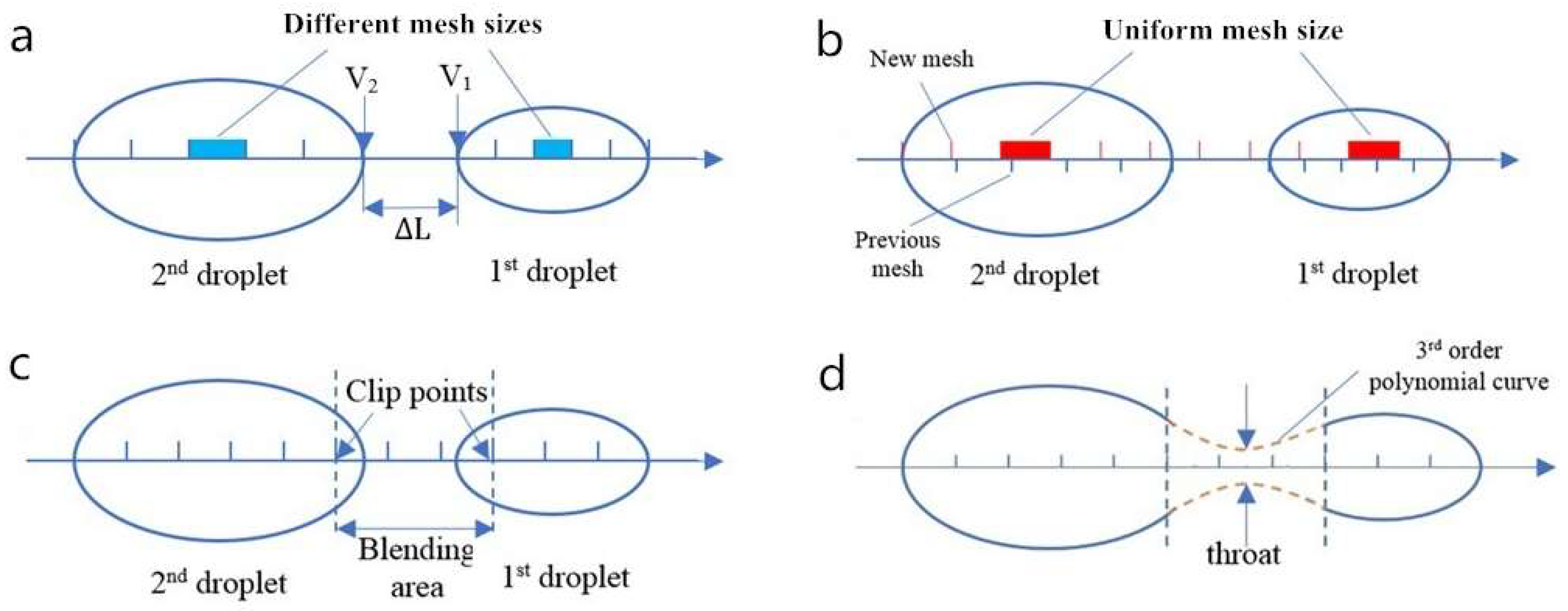
As shown in Figure 4a, v1, v2, dt, and ΔL in Equation (24) are velocity of the tail node in the first droplet, velocity of the head node in the second droplet, time step, and distance between two droplets, respectively. The coefficient of 0.8 in Equation (24) is chosen from our numerical tests. Note that although mesh is always evenly distributed in a droplet, different droplets usually have different mesh size due to the extension and the contraction during fluid motion. As a result, the whole space occupied by the merged droplet needs to be first remeshed with a uniform mesh size (i.e., the original mesh size dz0), as shown in Figure 4b. Similar to the case of the remeshing, due to the severe contraction and the extension, the shape-preserving piecewise cubic interpolation is also used to evaluate height and velocity at new nodes. After that, two nodes nearest to the approaching ends can be identified, as shown in Figure 4c. We call these two nodes clip points, because the area between them, namely the blending area, will be clipped out for shape reconstruction. The smoothness of the blending area is paramount for numerical stability [41], therefore, a third-order polynomial curve is used to construct a smooth contour in the blending area. It means that at least two more equations are needed to determine this curve except the clip points. These two equations are given by a throat which is located in the center of blending area, with a height of 1% of orifice radius r0 and a slope of zero. Figure 4d shows the result of drop coalescence with a highlight on the blending area and the throat. While this blending method is reliable and robust, it does add a small amount of mass into the system. We examined several instances, and found that the additional mass is less than 0.1% of the two merging droplets, and hence, is negligible.
3.4. Coupling of Nozzle Dynamics and Droplet Formation
Meniscus is the interface between the fluid in the nozzle and the ambient air. The meniscus can recede inside the nozzle or protrude out of the nozzle plane, as shown in Figure 5. When the extension of the liquid from the nozzle plane (i.e., the dashed line in Figure 5) is less than a threshold distance (i.e., the nozzle radius), the liquid motion can be solved just using the nozzle dynamics model (discussed in Section 2.2). However, if the liquid protrudes out of the nozzle beyond the threshold, the liquid motion outside the nozzle plane has to be solved using the droplet formation model (discussed in Section 2.1), whereas the liquid motion inside the nozzle is still solved by the nozzle dynamics model. As a result, the solution of droplet formation needs to be coupled with the solution of the nozzle dynamics.
The pressure porifice produced by the outer flow, i.e., meniscus and droplets, are taken into consideration for the calculation of the pressure gradient in the nozzle region [32]. porifice is the capillary pressure and can be determined by the shape of the outer flow. The non-dimensional pressure gradient in the nozzle region can be obtained by
Then with the help of Equation (17), the velocity profile in the nozzle can be obtained, which in turn will be applied as the boundary condition for the droplet formation model. A detailed flow chart of the coupling method of the nozzle dynamics and the droplet formation is shown in Figure 6.
Although the accurate shape of meniscus demands many points along radial direction to depict, we only use a segment of the sphere determined by the position of vertex to represent it, as shown in Figure 5b. This simplification can greatly ease the calculation, because we only need to consider the centerline velocity v*center and the capillary pressure porifice at the orifice plane.
The RN and RT and a in Equation (27) are the normal and tangential principle radius of meniscus, as well as the extension of vertex. Equation (28) is the Young–Laplace equation.
Nevertheless, a segment of the sphere is unable to represent the meniscus if the displacement of the vertex inside the nozzle is larger than the orifice radius, such as the case in Figure 5a. Actually, this scenario often occurs at the beginning of the driving pressure wave, where a strong negative pressure sucks the meniscus into the nozzle. As a result, in this case, we switch to a hemi-ellipsoid to represent the meniscus. The expression of RN and RT are given in Equation (29).
When the extension of the vertex outside the nozzle plane is equal to the orifice radius, i.e., the shape of meniscus reaches a positive hemisphere, it triggers the coupling of the droplet formation and nozzle dynamics. At this moment, for the droplet formation model, the initial condition is provided by the discretization of the meniscus hemisphere in a uniform staggered mesh and the assumption that the hemisphere moves uniformly with the mean velocity, and the boundary condition is always determined by the mean velocity at the orifice v*mean.
4. Numerical Tests
In this section, we present four numerical tests to validate our 1D model. The first example is an infinite microthread under different sinusoidal perturbation. The second example involves a single sphere droplet flying without any disturbance, aiming to evaluate the calculation of surface tension and the conservation of the mass and momentum. The third example is a contracting filament with different Ohnesorge number. The fourth example is a DOD inkjet under a step driving pressure to check the overall performance of the 1D simulation. The numerical results are compared with established simulation data available from the literature and the high fidelity 2D axisymmetric simulations using our in-house developed code which has been used in modeling of various surface-tension driven flows in inkjet technologies [27,50,51,52,53].
4.1. Infinite Microthread
Since Rayleigh’s linear theory [54], the stationary infinite thread of liquid with harmonic disturbance has become a standard model to investigate the temporal instability of a liquid jet [55], because the behavior of the jets is substantially independent of the forward motion common to all its parts [56]. A lot of data has been established by previous publications. Here, we compare the breakup time predicted from our code with Ashgriz’s 2D finite element simulation [55] and Furlani’s 1D finite difference simulation [42].
With wavelength λ, scaled wavenumber k+ = 2πr0/λ and amplitude ratio ε, the shape of the microthread is described by
Instead of using the Oh number in our equations of motion (9), Ashgriz and Furlani adopt the Re number to determine the property of the microthread. Actually, they are equivalent, viz. the Re number is the reciprocal of the Oh number, because the microthread is stationary and the capillary velocity vc is applied into the Re number.
A series of scaled time t+ = t/tc (capillary time tc = (ρr03/σ)1/2) of breakup are obtained with different k+ and Re under ε = 0.05. Table I lists the breakup times predicted from our simulations, as well as Ashgriz’s [55] and Furlani’s [42] simulations. A very good agreement between our study and these published studies can be found from Table 1. Figure 7 shows the evolution of the droplet profile at the breakup moment and post-breakup for k+ = 0.7 and Re = 10.
4.2. Free Flying Droplet
The DOD inkjet is a surface-tension dominated flow [22,27]. The calculation of the surface tension on the free surface is critical to the successful modeling of the droplet ejection process. To test how well our model deals with the surface tension as well as the conservation of the mass and the momentum, we carry out a simulation of a sphere droplet flying straight without any disturbance. Because we neglect the drag force caused by the air, the exact solution is straightforward, i.e., the sphere droplet should keep its spherical shape and have a uniform linear motion. Therefore, by monitoring the mass, the momentum, and the droplet shape during numerical solution, we can easily evaluate the accuracy of the surface-tension calculation and the numerical algorithm proposed in this study.
The initial velocity and radius of droplet is set as v0 = 10 m/s, r0 = 10 μm, and Oh = 0.01. To check the mesh convergence, three mesh sizes (i.e., the number of nodes are 51, 101, and 201, respectively) are applied. The time histories of the momentum and the mass of the flying droplet are plotted in Figure 8c,d, respectively. Note that the y axis is the deviation compared with analytical solution with unit of ‰. We can find that even for the coarsest mesh, the error is less than 0.3‰. The momentum increases very slightly at the beginning and then becomes stable. When the mesh size is refined further, the momentum is almost strictly conserved in the whole motion. The sphere shape of droplet is also very well maintained in the entire process for all mesh sizes. The shape at t+ = 1 and t+ = 2 for mesh size of 101 nodes are shown in Figure 8a,b. It is clear from Figure 8 that the droplet shape is identical to the initial shape.
4.3. Liquid Filament Contraction
When the droplet pinches off from the orifice of a DOD inkjet device, the droplet is a nearly symmetrical filament about its equatorial midplane [44]. Therefore, the study on the contracting liquid filament can give insight on how satellite (secondary) droplets are formed, which is of great importance in inkjet printing. The most widely studied filament shape comprises an axisymmetric cylinder body and two hemispherical cap at both ends, and is initially taken to be at rest [57]. Thus a test on the contraction of this kind of filament can shed some light on the performance of our 1D model in predicting the evolution of satellite droplets. Since there are only two parameters governing this problem [44], the aspect ratio α = L0/2r0 (where L0 and r0 is the length and radius of the filament, respectively), and the Oh number. In this test, a short filament and a long filament are examined respectively, and three Oh numbers are applied in the long filament. The results are compared with the 2D axisymmetric simulations which are carried out using the modified open-source code Gerris [27].
When the filament is short and the viscosity is not very high, it will ultimately contract into a sphere and oscillate several times before reaching the stable state. The parameters for the short filament are α = 4.5 and Oh = 0.1. Figure 9a plots the initial filament shape and the final liquid shape after contraction. As expected, for the short filament, the liquid filament collapses into a perfect spherical droplet. The time histories of filament length predicted from 1D and 2D simulations are shown in Figure 9b, where y axis is the scaled length L+ = L/r0. It is clear that the 1D simulation result agrees very well with the 2D simulation during the contracting phase. The result from the 1D model begins to diverge from that predicted by the 2D model during the oscillation stage. This is because of the large vorticity generated during oscillation, which makes the 1D assumption invalid [44,58].
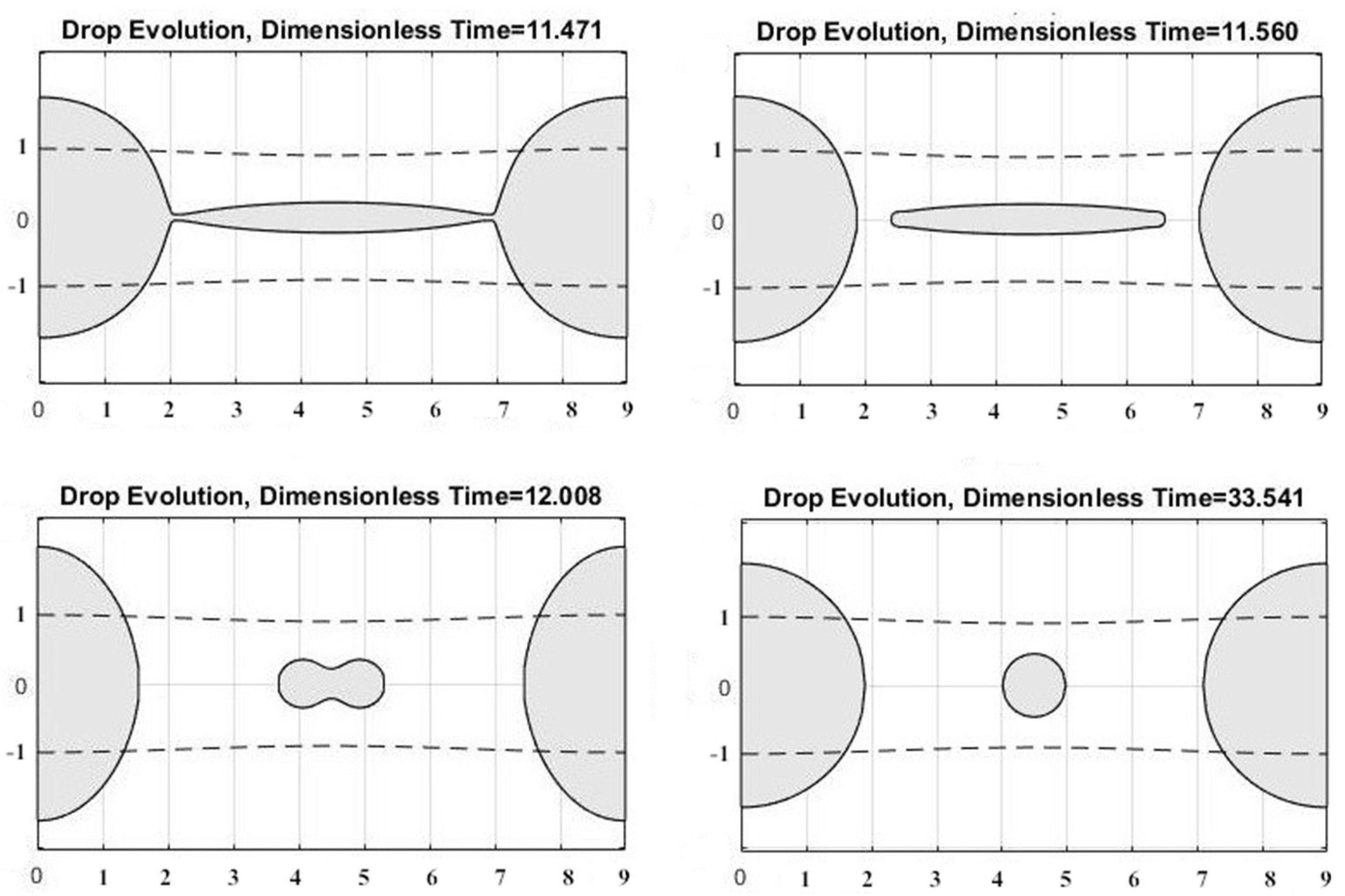
For a long filament, behavior varies with the Oh number. With a low Oh number (i.e., strong surface tension and weak viscosity), the long filament tend to breakup at the tip in contraction and produce multiple droplets in the end, instead of recoiling into a single droplet in the high Oh number scenario. Thus, similar simulations are carried out using a large aspect ratio α = 15 and Oh = 0.1, 0.01, and 0.001. Both 1D and 2D simulation results show that the filament breaks up in Oh number of 0.01 and 0.001, which agrees, very well, with Castrejon-Pita’s experimental result [59] and Hoath’s critical aspect ratio of 4.2 for low viscosity fluid [60]. The comparison of the evolution of the filament shape predicted by the 1D and 2D simulations is shown in Figure 10a,c,d,e,g. Since the liquid filament for cases of Oh = 0.01 and 0.001 eventually breaks up into multiple droplets, we only plot the entire evolution of the filament for Oh = 0.1.
It is clear that the dashed line (2D simulations) and the solid line (1D simulations) are almost axisymmetric to each other in Figure 10a,c,e,g. It is noticeable that there are some differences in Figure 10d for Oh = 0.1. The filament predicted by the 2D method contracts more intensively than that from 1D solution, and has an overturned surface when t+ = 16 and 17. This is caused by the intrinsic limitation of the 1D method, i.e., the inability to describe a multivalued curve. The comparisons of the filament length predicted by the 1D and 2D simulations for different Oh numbers are shown in Figure 10b,f,h. It is observed that the red line with circle mark (1D) nearly overlaps the blue line with triangle mark (2D) in most of the solution time.
4.4. Step Driving Pressure
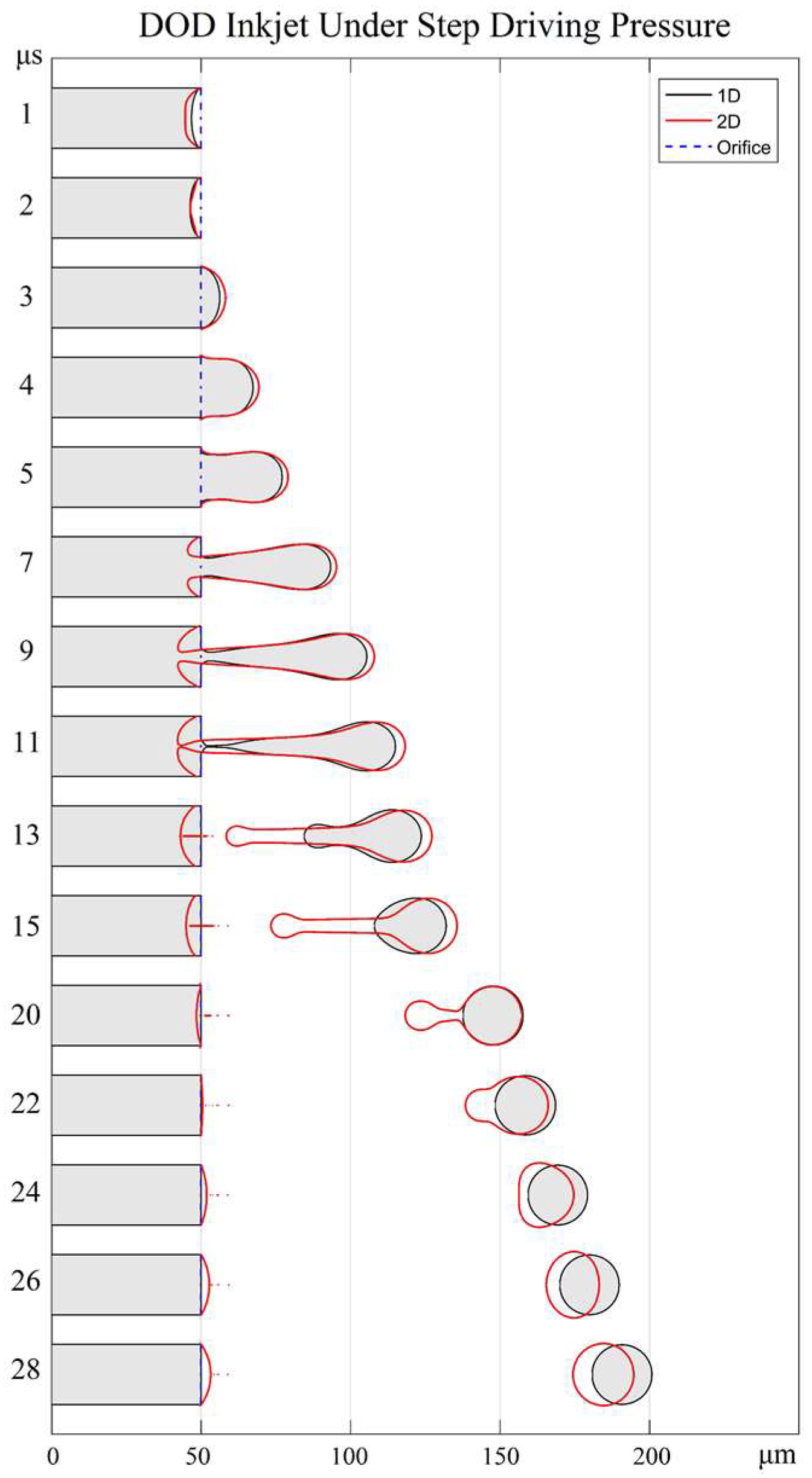
To validate the overall performance of our 1D model for an inkjet process, a droplet ejection is simulated with 1D model with real nozzle dimensions of r0 = 10 μm, Ln = 50 μm. Ink properties are ρ = 1.135 g/cm3, σ = 67.26 dyn/cm, μ = 0.0615 P. A simplified step driving pressure (shown in Table 2 and Figure 11) is employed in the test, which is used by Fromm [34] and Adams [32], as well. The results are compared with the 2D simulation.
The comparison of the evolutions of droplet ejection between 1D and 2D simulations are shown in Figure 12. As shown in Figure 12, there is a very good agreement between the 1D and 2D methods in the first 5 μs in terms of the meniscus movement and droplet formation. This indicates that the simplification of meniscus shape mentioned in Section 3.4 is a reasonable approximation for the droplet ejection in DOD inkjet technologies. A noticeable difference begins to appear after 7 μs. The meniscus of the 2D method has an overturned surface around the orifice, which cannot be described by the1D method. However, the droplet shape out of the orifice plane from 1D simulation is in a good agreement with that from 2D simulation. Besides, it is noteworthy that both models predict nearly the same droplet pinch-off time of ~11 μs, which demonstrates a good temporal accuracy of the 1D method. At 20 μs, the relative position of both droplets changes. Due to its longer tail and larger mass, the droplet predicted by the 2D method is surpassed by that of the 1D method. As the two methods predict a slight difference in terminal velocity, the distance between them keeps increasing after 28 μs.
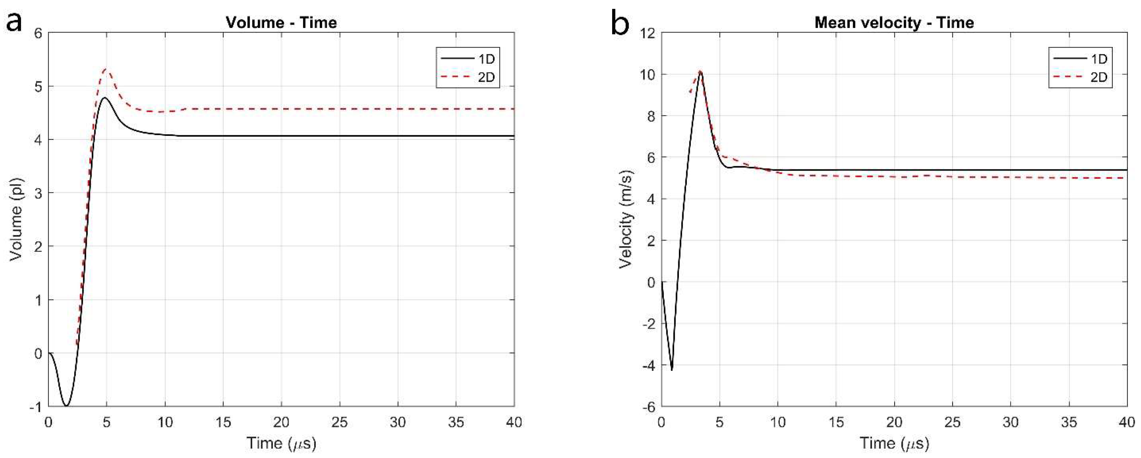
The time history of the accumulative liquid volume from the orifice plane predicted by the 1D simulation is compared with that by the 2D simulation as shown in Figure 13a. The final volume in each curve of Figure 13a indicates the final droplet volume, which is 4.06 pL for the 1D simulation and 4.56 pL for the 2D simulation. The 11% difference between the 1D and 2D methods is acceptable, given the fact that the inevitable mass loss is caused by the overturned surface in the 1D method. The time histories of the average velocity of the droplet during ejection process predicted from the two methods are plotted in Figure 13b. It is clear that there is a very good agreement in droplet velocity between the two methods during the initial ejection phase. The 1D method predicts the final velocity as 538 cm/s, whereas the 2D method has a final average velocity of 492 cm/s. Given the same driving pressure, the smaller mass predicted by the 1D results in a slightly higher final velocity.
We also need to point out that the 1D simulation takes less than one minute to finish, whereas a 2D asymmetrical simulation takes about 18 min. The significant advantage of 1D model over 2D model in terms of computational cost makes the 1D model a very useful tool for the massive screening and optimization for inkjet devices.
5. Example of Droplet Ejection Simulation
In reality, the driving pressure of printhead is a damping sinusoidal wave instead of a simple step function. For the squeeze mode PIJ, the pressure waveform is usually the superposition of two waves: 1. a negative wave caused by the charging of PZT which is then reflected into a positive wave by the ink reservoir; 2. a positive wave result from the de-charging of PZT used to amplify the reflected wave [61]. To demonstrate the capability of our 1D model in dealing with the real inkjet condition and the effect of Oh number on the droplet formation, a typical PIJ pressure waveforms (as shown in Figure 14) is applied to the nozzle inlet and fluid properties are given as ρ = 1 g/cm3, σ = 40 dyn/cm, μ = 0.2 cP, 1 cP, 2 cP corresponding to Oh = 0.01, 0.05, 0.1. The nozzle dimensions are r0 = 10 μm, Ln = 50 μm. The waveform starts from a negative pressure with the minimum of −1.23 Mpa and the duration of 1.1 μs. At 2.0 μs, the first waveform is amplified by a higher pressure, reaching the extremum of 2.19 Mpa and −1.76 Mpa at 2.3 μs and 4.0 μs, respectively. Finally, the pressure waves are damped to zero.
Figure 15 shows the droplet ejection process with three different Oh numbers. The times of pinching off from the orifice are 5.3 μs, 5.4 μs, and 6.4 μs for Oh = 0.01, 0.05, and 0.1, respectively. The higher viscosity leads to a longer pinch-off time of the ligament, which is in agreement of Dong et al.’s experimental study [62]. In the case of Oh = 0.01, the droplet experienced large oscillation after being pinched off from the orifice, due to the low viscosity. On the contrary, in the highest viscosity case (i.e., Oh = 0.1), the main droplet almost did not oscillate much, and had a satellite droplet following it. However, due to the higher velocity, the satellite droplet caught up and merged with the main droplet at 16.1μs. In the case of modest viscosity (i.e., Oh = 0.05), surface tension and viscosity are balanced, thus, the oscillation is damped fast and no satellite droplet is produced.
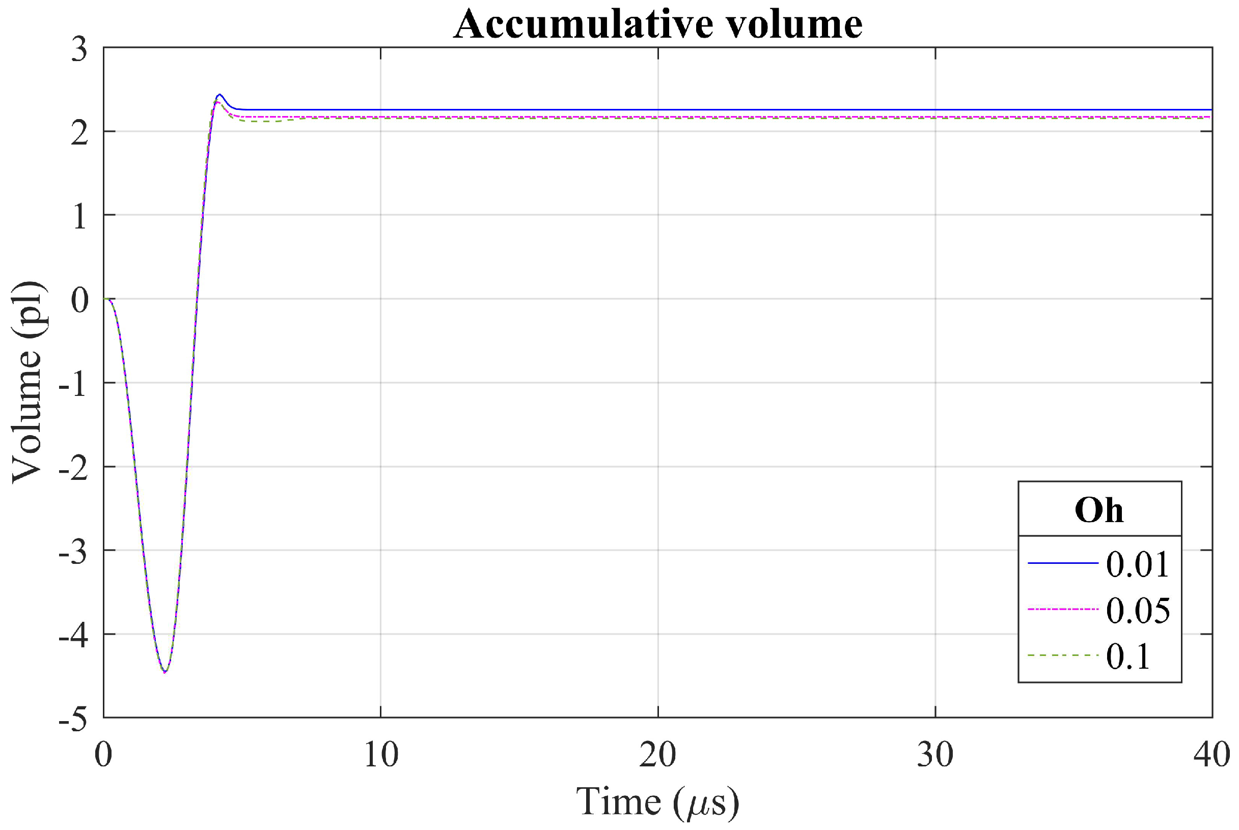
Figure 16 plots the accumulative volume of the three ejections. The total volume in Oh = 0.01, 0.1, and 0.5 are 2.254 pL, 2.170 pL, and 2.053 pL, respectively. The droplet velocity for three Oh numbers are 7.8 m/s, 7.1 m/s, and 6.2 m/s, respectively. The decreased mass is the result of the increased viscosity. This result is also consistent with Dong et al.’s experimental study [62].
6. Conclusions
A 1D numerical simulation of droplet ejection in DOD inkjet is presented in this paper. The whole process is divided into two coupled models: droplet formation and nozzle dynamics. Only the liquid phase is considered in the droplet formation model. The NS equations are reduced into two coupled 1D PDEs by the slender jet analysis. The governing equations are discretized by a uniform staggered mesh and solved by a finite-difference based ALE method. The fluid dynamics in the nozzle are described by the 2D axisymmetric unsteady Poiseuille flow, in which an analytical solution can be found. The droplet formation and the nozzle dynamics are coupled together once the meniscus extends from the orifice plane beyond the threshold value. Numerical treatment of the droplet ends, and the breakup location is proposed to avoid the singularity of the curvature calculation at these locations. The shape-preserving piecewise cubic interpolation and third-order polynomial curve are employed to treat the coalescence of multiple droplets during solution. These algorithms are implemented in an in-house developed MATLAB code.
Four numerical tests are carried out to comprehensively evaluate the performance of the 1D model for inkjet process. The breakups of an infinitely long microscopic liquid thread with different initial perturbations are first solved by the 1D model. The results show great agreement with previously published data. Then, the accuracy of the surface-tension calculation in the 1D model is proven in the example of a free flying droplet, in which the momentum and the mass are conserved very well with a very stable droplet profile. For the contracting liquid filament, the simulation results from the 1D model are compared against the 2D axisymmetric simulations. During the contracting phase, the evolution of the filament shape predicted by 1D and 2D methods is almost identical, whereas in the oscillation phase the droplet in the 1D method shows faster damping rate, due to the intrinsic limitation of the 1D method. The last test example is a 1D simulation of the droplet ejection under a simple step driving pressure. Close agreement of droplet shape and breakup time between 1D and 2D methods are found in this test. Finally, droplet ejections under a more realistic sinusoidal pressure waveform and with three different Oh number are presented to show the effect of Oh number on the droplet ejection. The simulations presented in this paper usually take less than one minute, which makes it very useful to quickly explore large design parameters of inkjet devices, including nozzle geometry, fluid properties, operation conditions (e.g., frequency, pressure waveform, etc.).
Acknowledgments
The authors would like to thank the Office of Research Support & Operations of Washington State University (WSU) for their support through the New Faculty Seed Grant Program (#128044-001). We also would like to thank the Office of Academic Affairs of WSU-Vancouver for additional financial support. The work is funded in part by US National Science Foundation award CBET-1701339.
Author Contributions
H.T. proposed the coupling algorithm and validation examples used in the paper; H.J. developed the simulation code and analyzed the data; H.J. and H.T. wrote the paper together.
Conflicts of Interest
The authors declare no conflict of interest.
References
- Calvert, P. Inkjet Printing for Materials and Devices. Chem. Mater. 2001, 13, 3299–3305. [Google Scholar] [CrossRef]
- Thomas, H.R.; Hopkinson, N.; Erasenthiran, P. High speed sintering—continuing research into a new rapid manufacturing process. In Proceedings of the 17th SFF Symposium, Austin TX, USA, 14–16 August 2006; pp. 682–691. [Google Scholar]
- Yoshihiro, K.; Hodges, S.; Cook, B.S.; Zhang, C.; Abowd, G.D. Instant inkjet circuits: Lab-based Inkjet Printing to Support Rapid Prototyping of UbiComp Devices. In Proceedings of the 2013 ACM International Joint Conference on Pervasive and Ubiquitous Computing, Zurich, Switzerland, 08–12 September 2013; pp. 363–372. [Google Scholar] [CrossRef]
- Daly, R.; Harrington, T.S.; Martin, G.D.; Hutchings, I.M. Inkjet printing for pharmaceutics—A review of research and manufacturing. Int. J. Pharm. 2015, 494, 554–567. [Google Scholar] [CrossRef] [PubMed]
- Derby, B. Printing and prototyping of tissues and scaffolds. Science 2012, 338, 921–926. [Google Scholar] [CrossRef] [PubMed]
- Bash, C.E.; Patel, C.D.; Sharma, R.K. Inkjet assisted spray cooling of electronic. In Proceedings of the ASME 2003 International Electronic Packaging Technical Conference and Exhibition, Maui, Hawaii, USA, 6–11 July 2003; Volume 2, pp. 119–127. [Google Scholar]
- Hoath, S.D. Fundamentals of Inkjet Printing: The Science of Inkjet and Droplets; John Wiley & Sons: Hoboken, NJ, USA, 2016. [Google Scholar]
- Dong, H.; Carr, W.W.; Morris, J.F. Visualization of drop-on-demand inkjet: Drop formation and deposition. Rev. Sci. Instrum. 2006, 77, 085101. [Google Scholar] [CrossRef]
- Hutchings, I.M.; Martin, G.D.; Hoath, S.D. High speed imaging and analysis of jet and drop formation. J. Imaging Sci. Technol. 2007, 51, 438–444. [Google Scholar] [CrossRef]
- Van der Bos, A.; van der Meulen, M.J.; Driessen, T.; van den Berg, M.; Reinten, H.; Wijshoff, H.; Versluis, M.; Lohse, D. Velocity profile inside piezoacoustic inkjet droplets in flight: Comparison between experiment and numerical simulation. Phys. Rev. Appl. 2014, 1, 014004. [Google Scholar] [CrossRef]
- Staat, H.J.J.; van der Bos, A.; van den Berg, M.; Reinten, H.; Wijshoff, H.; Versluis, M.; Lohse, D. Ultrafast imaging method to measure surface tension and viscosity of inkjet-printed droplets in flight. Exp. Fluids 2017, 58. [Google Scholar] [CrossRef]
- Fromm, J.E. Numerical Calculation of the Fluid Dynamics of Drop-on-Demand Jets. IBM J. Res. Dev. 1984, 28, 322–333. [Google Scholar] [CrossRef]
- Morrison, N.F.; Harlen, O.G. Viscoelasticity in inkjet printing. Rheol. Acta 2010, 49, 619–632. [Google Scholar] [CrossRef]
- Castrejón-Pita, J.R.; Morrison, N.F.; Harlen, O.G.; Martin, G.D.; Hutchings, I.M. Experiments and Lagrangian simulations on the formation of droplets in drop-on-demand mode. Phys. Rev. E 2011, 83, 036306. [Google Scholar] [CrossRef] [PubMed]
- Castrejon-Pita, J.R.; Morrison, N.F.; Harlen, O.G.; Martin, G.D.; Hutchings, I.M. Experiments and Lagrangian simulations on the formation of droplets in continuous mode. Phys. Rev. E 2011, 83, 16301. [Google Scholar] [CrossRef] [PubMed]
- Morrison, N.F.; Harlen, O.G.; Hoath, S.D. Towards satellite free drop-on-demand printing of complex fluids. In 2014 International Conference on Digital Printing Technologies; Society for Imaging Science and Technology: Springfield, VA, USA, 2014; pp. 162–165. [Google Scholar]
- Knight, B. Computer modeling of a thermal inkjet device. In IS&T Seventh International Congress on Advances in Non-Impact Printing Technologies; Society for Imaging Science: Springfield, VA, USA, 1991. [Google Scholar]
- Asai, A. Three-Dimensional Calculation of Bubble Growth and Drop Ejection in a Bubble Jet Printer. J. Fluids Eng. 1992, 114, 638. [Google Scholar] [CrossRef]
- Liou, T.M.; Shih, K.C.; Chau, S.W.; Chen, S.C. Three-dimensional simulations of the droplet formation during the inkjet printing process. Int. Commun. Heat Mass Transf. 2002, 29, 1109–1118. [Google Scholar] [CrossRef]
- Wu, H.-C.; Hwang, W.-S.; Lin, H.-J. Development of a three-dimensional simulation system for micro-inkjet and its experimental verification. Mater. Sci. Eng. A 2004, 373, 268–278. [Google Scholar] [CrossRef]
- Wu, H.-C.; Lin, H.-J.; Kuo, Y.-C.; Hwang, W.-S. Simulation of Droplet Ejection for a Piezoelectric Inkjet Printing Device. Mater. Trans. 2004, 45, 893–899. [Google Scholar] [CrossRef]
- Tan, H.; Torniainen, E.; Markel, D.P.; Browning, R.N.K. Numerical simulation of droplet ejection of thermal inkjet printheads. Int. J. Numer. Methods Fluids 2015, 77, 544–570. [Google Scholar] [CrossRef]
- Yu, J.-D.; Sakai, S.; Sethian, J. A coupled level set projection method applied to ink jet simulation. Interfaces Free Bound. 2003, 5, 459–482. [Google Scholar] [CrossRef]
- Der Yu, J.; Sakai, S.; Sethian, J. A coupled quadrilateral grid level set projection method applied to ink jet simulation. J. Comput. Phys. 2005, 206, 227–251. [Google Scholar] [CrossRef]
- Suh, Y.; Son, G. A Level-Set Method for Simulation of a Thermal Inkjet Process. Numer. Heat Transf. Part B Fundam. 2008, 54, 138–156. [Google Scholar] [CrossRef]
- Harlen, O.G.; Morrison, N.F. Simulations of drop formation in complex rheological fluids-can rheology improve jetting performance? In NIP & Digital Fabrication Conference; Society for Imaging Science and Technology: Springfield, VA, USA, 2016; pp. 378–381. [Google Scholar]
- Tan, H. An adaptive mesh refinement based flow simulation for free-surfaces in thermal inkjet technology. Int. J. Multiph. Flow 2016, 82, 1–16. [Google Scholar] [CrossRef]
- Feng, J. A general fluid dynamic analysis of drop ejection in drop-on-demand ink jet devices. J. Imaging Sci. Technol. 2002, 46, 398–408. [Google Scholar]
- Sen, A.K.; Darabi, J. Droplet ejection performance of a monolithic thermal inkjet print head. J. Micromech. Microeng. 2007, 17, 1420–1427. [Google Scholar] [CrossRef]
- Lindemann, T.; Sassano, D.; Bellone, A.; Zengerle, R.; Koltay, P. Three-Dimensional CFD-Simulation of a Thermal Bubble Jet Printhead. In Proceedings of the NSTI Nanotechnology Conference and Trade Show, Boston, MA, USA, 7–11 March 2004; Volume 2, pp. 227–230. [Google Scholar]
- Zhou, H.; Gué, A.M. Simulation model and droplet ejection performance of a thermal-bubble microejector. Sens. Actuators B Chem. 2010, 145, 311–319. [Google Scholar] [CrossRef]
- Adams, R.L.; Roy, J. A One-Dimensional Numerical Model of a Drop-On-Demand Ink Jet. J. Appl. Mech. 1986, 53, 193. [Google Scholar] [CrossRef]
- Lee, H.C. Drop Formation in a Liquid Jet. IBM J. Res. Dev. 1974, 18, 364–369. [Google Scholar] [CrossRef]
- Fromm, J. A numerical study of drop-on-demand ink jets. In Proceedings of the 2nd International Colloquium on Drops and Bubbles, San Jose, CA, USA, 1 March 1982. [Google Scholar]
- Shield, T.W.; Bogy, D.B.; Talke, F.E. A numerical comparison of one-dimensional fluid jet models applied to drop-on-demand printing. J. Comput. Phys. 1986, 67, 327–347. [Google Scholar] [CrossRef]
- Green, A.E. On the non-linear behaviour of fluid jets. Int. J. Eng. Sci. 1976, 14, 49–63. [Google Scholar] [CrossRef]
- Wallace, D. A Method of Characteristics Model of a Drop-on-Demand Ink-Jet Device Using an Integral Method Drop Formation Model; ASME Publication: New York, NY, USA, 1989. [Google Scholar]
- Eggers, J.; Dupont, D.F. Drop formation in a one-dimensional approximation of the Navier-Stokes equation. J. Fluid Mech. 1994, 262, 205–221. [Google Scholar] [CrossRef]
- Ambravaneswaran, B.; Wilkes, E.D.; Basaran, O.A. Drop formation from a capillary tube: Comparison of one-dimensional and two-dimensional analyses and occurrence of satellite drops. Phys. Fluids 2002, 14, 2606–2621. [Google Scholar] [CrossRef]
- Yildirim, O.E.; Xu, Q.; Basaran, O.A. Analysis of the drop weight method. Phys. Fluids 2005, 17, 1–13. [Google Scholar] [CrossRef]
- Hanchak, M. One Dimensional Model of Thermo-Capillary Driven Liquid Jet Break-up with Drop Merging; University of Dayton: Dayton, OH, USA, 2009. [Google Scholar]
- Furlani, E.P.; Hanchak, M.S. Nonlinear analysis of the deformation and breakup of viscous microjets using the method of lines. Int. J. Numer. Methods Fluids 2011, 65, 563–577. [Google Scholar] [CrossRef]
- Van Hoeve, W.; Gekle, S.; Snoeijer, J.H.; Versluis, M.; Brenner, M.P.; Lohse, D. Breakup of diminutive Rayleigh jets. Phys. Fluids 2010, 22, 122003. [Google Scholar] [CrossRef]
- Notz, P.K.; Basaran, O.A. Dynamics and breakup of a contracting liquid filament. J. Fluid Mech. 2004, 512, 223–256. [Google Scholar] [CrossRef]
- Driessen, T.; Jeurissen, R.; Wijshoff, H.; Toschi, F.; Lohse, D. Stability of viscous long liquid filaments. Phys. Fluids 2013, 25, 062109. [Google Scholar] [CrossRef]
- Shin, D.Y.; Grassia, P.; Derby, B. Numerical and experimental comparisons of mass transport rate in a piezoelectric drop-on-demand inkjet print head. Int. J. Mech. Sci. 2004, 46, 181–199. [Google Scholar] [CrossRef]
- Lee, Y. Analytical solutions of channel and duct flows due to general pressure gradients. Appl. Math. Model. 2017, 43, 279–286. [Google Scholar] [CrossRef]
- Jiang, H.; Tan, H. One Dimensional Simulation of Droplet Ejection of Drop-on-Demand Inkjet; IMECE, ASME: Tampa, FL, USA, 2017. [Google Scholar]
- Schiesser, W. The Numerical Method of Lines: Integration of Partial Differential Equations; Elsevier: New York, NY, USA, 2012. [Google Scholar]
- Tan, H. Numerical study on splashing of high-speed microdroplet impact on dry microstructured surfaces. Comput. Fluids 2017, 154, 142–166. [Google Scholar] [CrossRef]
- Tan, H. Absorption of picoliter droplets by thin porous substrates. AIChE J. 2017, 63, 1690–1703. [Google Scholar] [CrossRef]
- Kong, X.; Xi, Y.; LeDuff, P.; Li, E.; Liu, Y.; Cheng, L.-J.; Rorrer, G.L.; Tan, H.; Wang, A.X. Optofluidic sensing from inkjet-printed droplets: The enormous enhancement by evaporation-induced spontaneous flow on photonic crystal biosilica. Nanoscale 2016, 8, 17285–17294. [Google Scholar] [CrossRef] [PubMed]
- Tan, H. Three-dimensional simulation of micrometer-sized droplet impact and penetration into the powder bed. Chem. Eng. Sci. 2016, 153, 93–107. [Google Scholar] [CrossRef]
- Rayleigh, L. On the instability of jets. Proc. Lond. Math. Soc. 1878, s1-10, 4–13. [Google Scholar] [CrossRef]
- Ashgriz, N.; Mashayek, F. Temporal analysis of capillary jet breakup. J. Fluid Mech. 1995, 291, 163–190. [Google Scholar] [CrossRef]
- Strutt, J.W. The Theory of Sound; Cambridge University Press: London, UK, 2011; Volume 2. [Google Scholar] [CrossRef]
- Schulkes, R.M.S.M. The contraction of liquid filaments. J. Fluid Mech. 1996, 309, 277. [Google Scholar] [CrossRef]
- Hoepffner, J.; Paré, G. Recoil of a liquid filament: Escape from pinch-off through creation of a vortex ring. J. Fluid Mech. 2013, 734, 183–197. [Google Scholar] [CrossRef]
- Castrejón-Pita, A.A.; Castrejón-Pita, J.R.; Hutchings, I.M. Breakup of Liquid Filaments. Phys. Rev. Lett. 2012, 108, 74506. [Google Scholar] [CrossRef] [PubMed]
- Hoath, S.D.; Jung, S.; Hutchings, I.M. A simple criterion for filament break-up in drop-on-demand inkjet printing. Phys. Fluids 2013, 25, 021701. [Google Scholar] [CrossRef]
- Wijshoff, H. The dynamics of the piezo inkjet printhead operation. Phys. Rep. 2010, 491, 77–177. [Google Scholar] [CrossRef]
- Dong, H.; Carr, W.W.; Morris, J.F. An experimental study of drop-on-demand drop formation. Phys. Fluids 2006, 18, 072102. [Google Scholar] [CrossRef]
Figure 1.
Schematics of inkjet systems: (a) continuous inkjet (CIJ) inkjet; (b) drop-on-demand (DOD) inkjet.
Figure 1.
Schematics of inkjet systems: (a) continuous inkjet (CIJ) inkjet; (b) drop-on-demand (DOD) inkjet.

Figure 2.
Uniform staggered mesh of droplet formation: a droplet connecting to the nozzle.
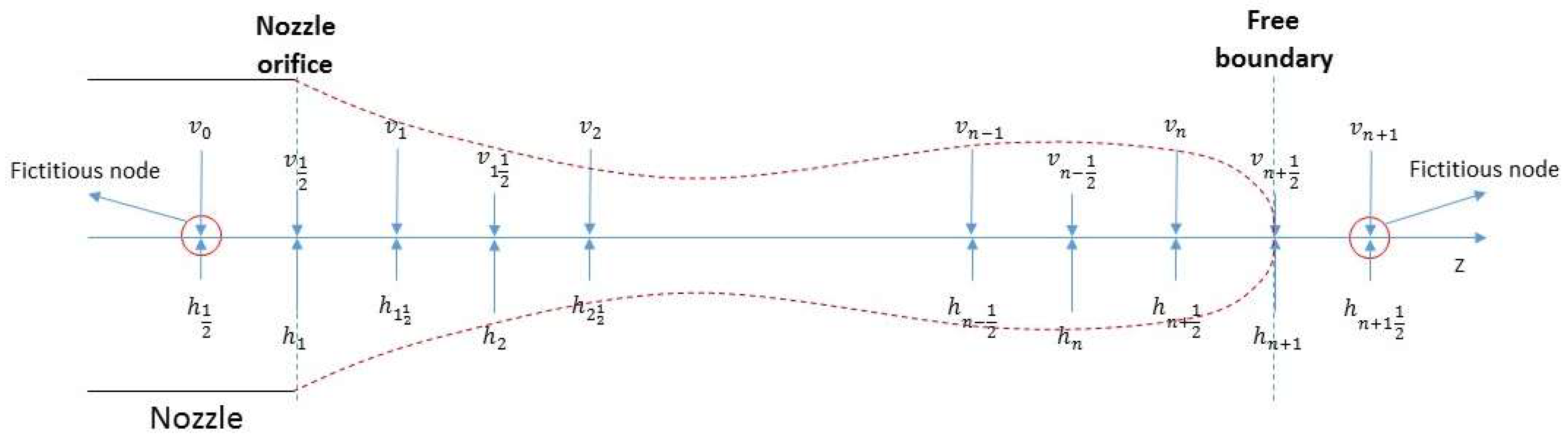
Figure 3.
Schematic of droplet breakup.
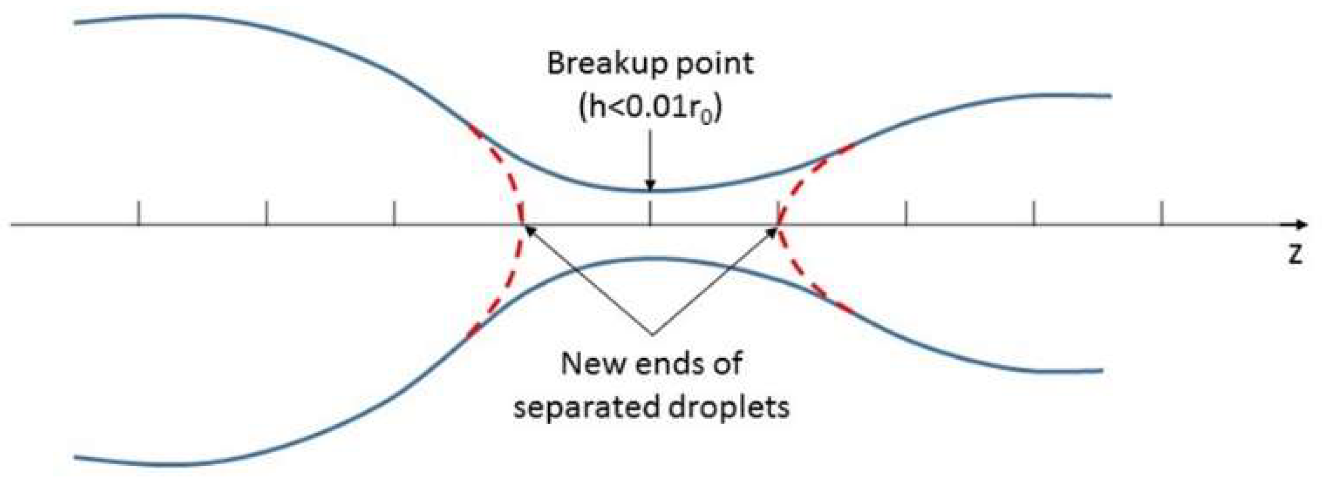
Figure 4.
Numerical procedure of droplet coalescence: (a) Two approaching droplets with different mesh sizes; (b) Remesh the whole space occupied by the merged droplet with a uniform mesh size; (c) Find clip points and blending area; (d) A merged droplet after the reconstruction of blending area.
Figure 4.
Numerical procedure of droplet coalescence: (a) Two approaching droplets with different mesh sizes; (b) Remesh the whole space occupied by the merged droplet with a uniform mesh size; (c) Find clip points and blending area; (d) A merged droplet after the reconstruction of blending area.

Figure 5.
Different stages of meniscus: (a) Hemi-ellipsoid: the extension of vertex is less than the negative orifice radius, due to negative driving pressure at the start of a pulse; (b) Segment of sphere: the extension of vertex is shorter than the positive orifice radius; (c) First coupling moment: the extension of vertex reaches positive orifice radius, and the hemisphere is discretized by a uniform staggered mesh. The boundary condition of droplet formation model is the mean velocity at nozzle orifice. The blue dashed line is the position of orifice plane, and the red circle is the position of vertex.
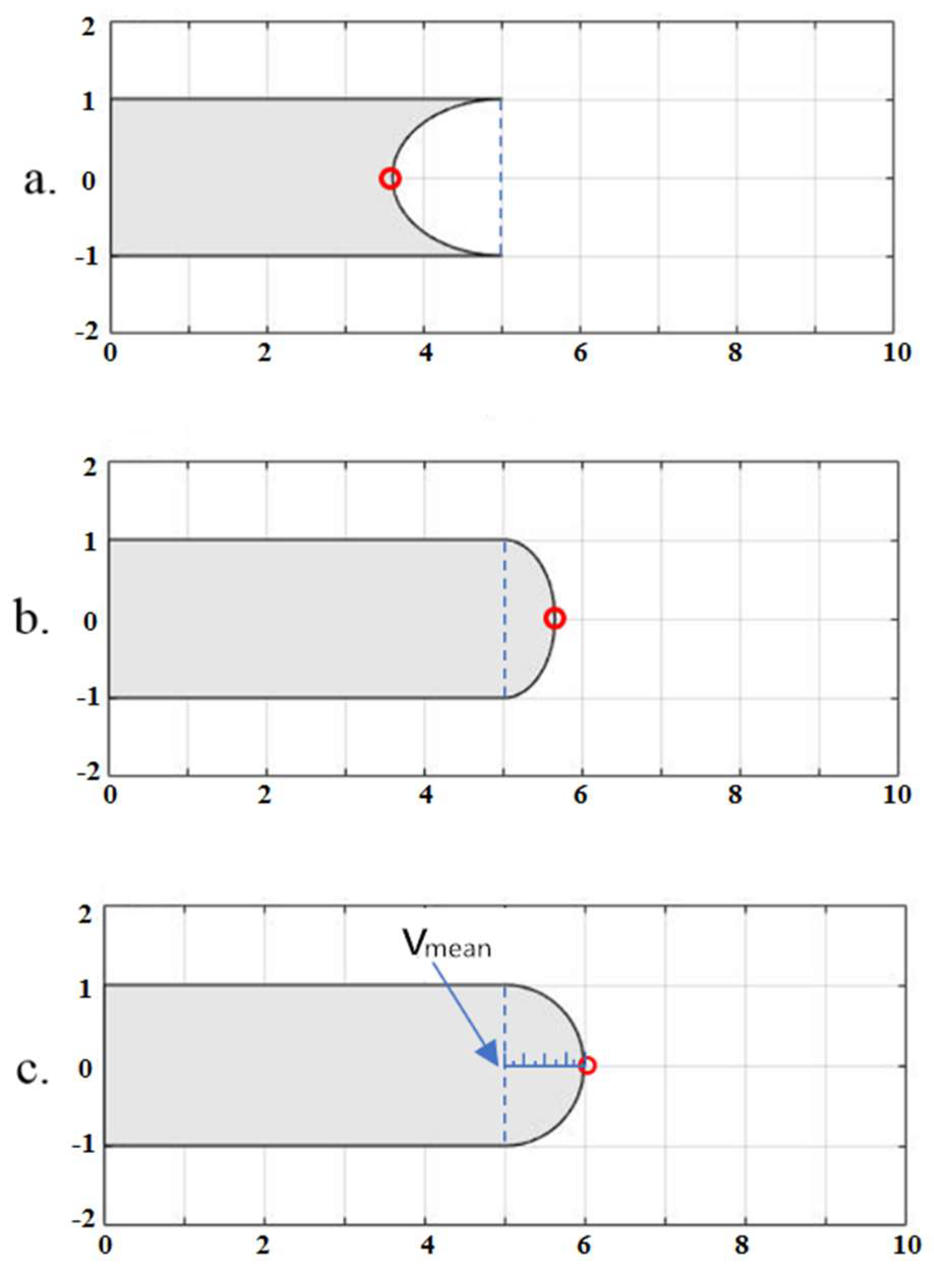
Figure 6.
Flow chart of 1D simulation of droplet ejection in DOD inkjet.
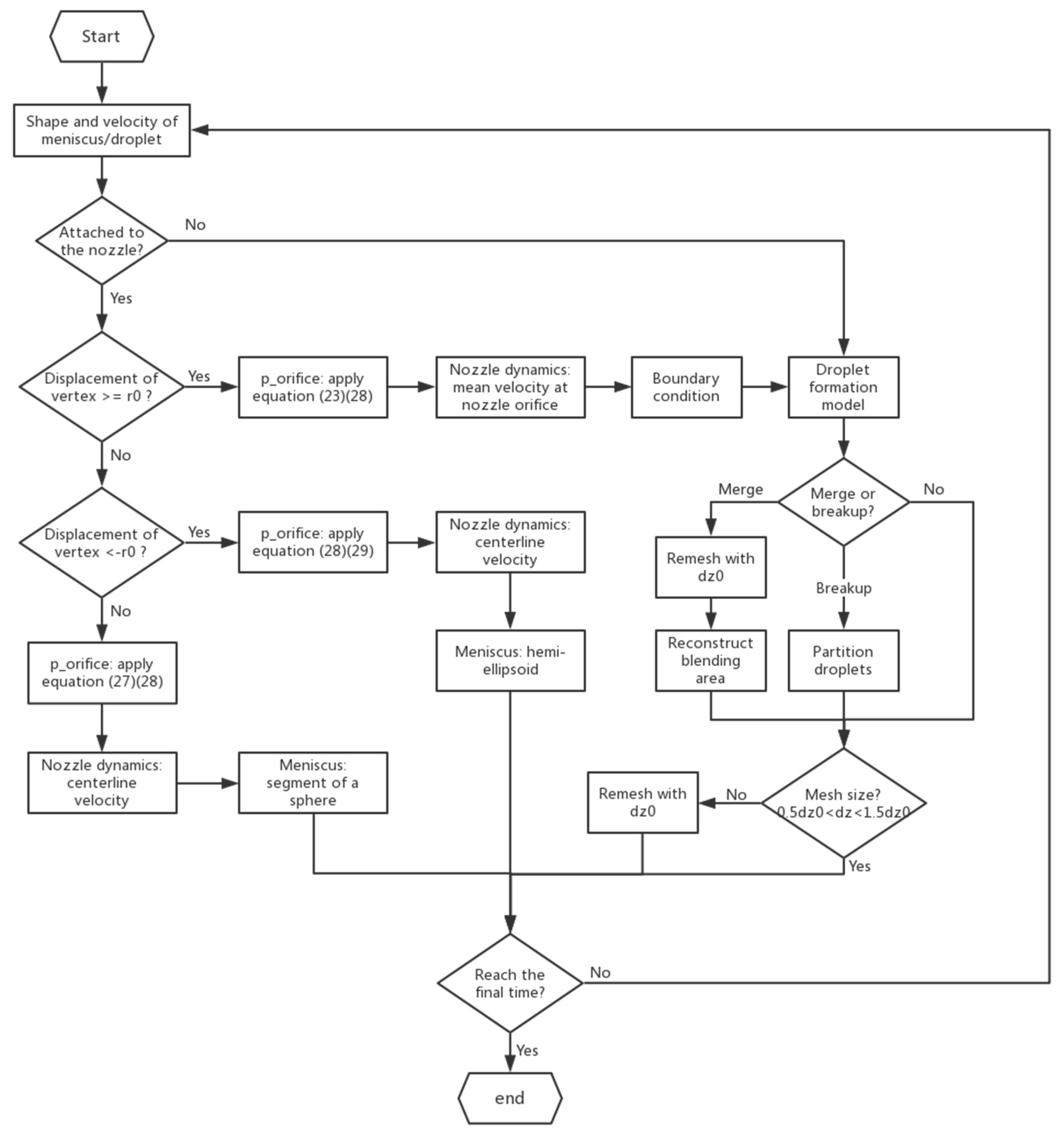
Figure 7.
Evolution of an infinite microthread under harmonic perturbation (k+ = 0.7, Re = 10, ε = 0.05): (a) Breakup moment; (b–d) Post-breakup moments. The dash line represents initial shape of the microthread.
Figure 7.
Evolution of an infinite microthread under harmonic perturbation (k+ = 0.7, Re = 10, ε = 0.05): (a) Breakup moment; (b–d) Post-breakup moments. The dash line represents initial shape of the microthread.

Figure 8.
Single sphere droplet flying without disturbance: (a) Droplet shape at t+ = 1; (b) Droplet shape at t+ = 2; (c) Momentum history; (d) Mass history.
Figure 8.
Single sphere droplet flying without disturbance: (a) Droplet shape at t+ = 1; (b) Droplet shape at t+ = 2; (c) Momentum history; (d) Mass history.
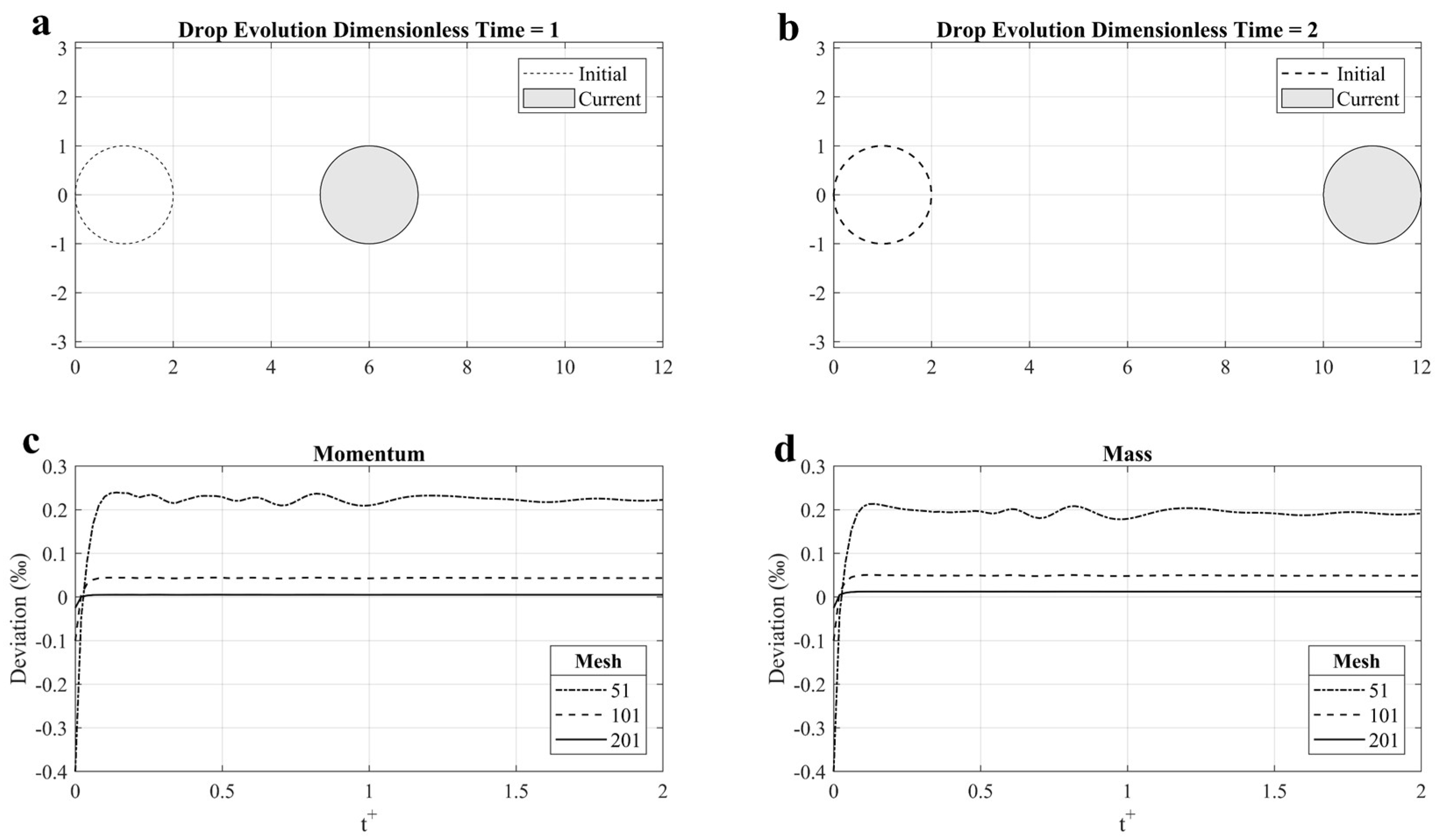
Figure 9.
Short filament contraction (α = 4.5, Oh = 0.1): (a) Comparison of initial and current shape; (b) Comparison of time histories of the filament length between 1D and 2D simulations.
Figure 9.
Short filament contraction (α = 4.5, Oh = 0.1): (a) Comparison of initial and current shape; (b) Comparison of time histories of the filament length between 1D and 2D simulations.
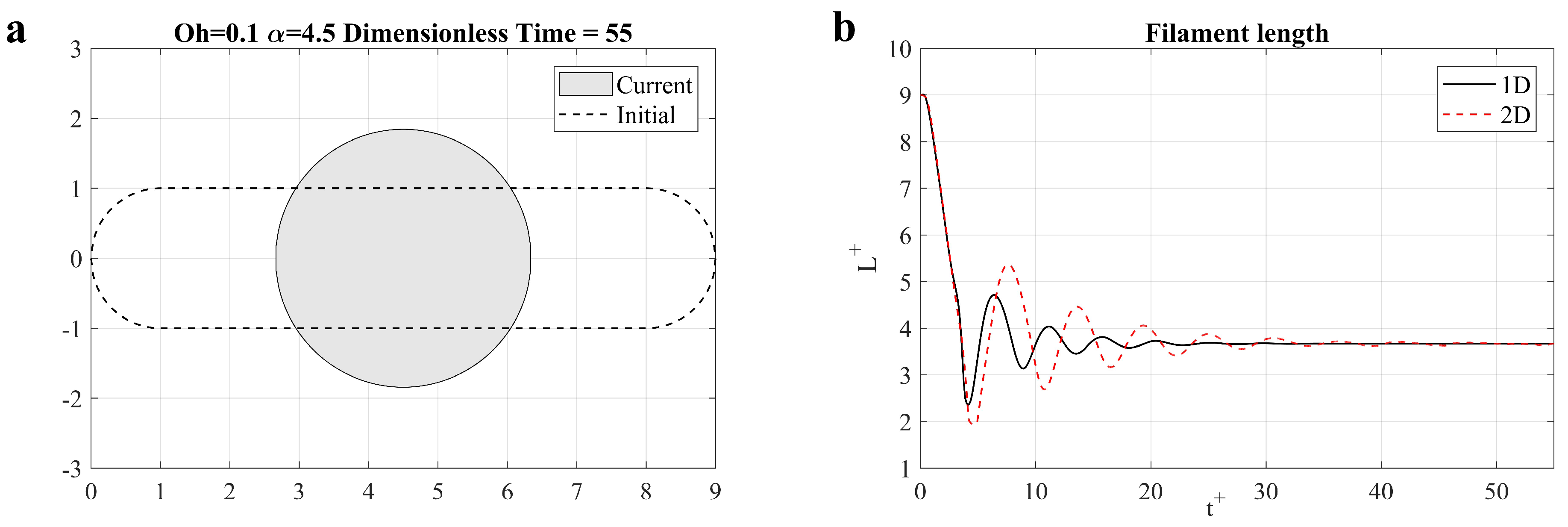
Figure 10.
Contraction of long liquid filament: (a,c,d,e,g) Shape evolution with different Oh; (b,f,h) Filament length vs time with different Oh.
Figure 10.
Contraction of long liquid filament: (a,c,d,e,g) Shape evolution with different Oh; (b,f,h) Filament length vs time with different Oh.
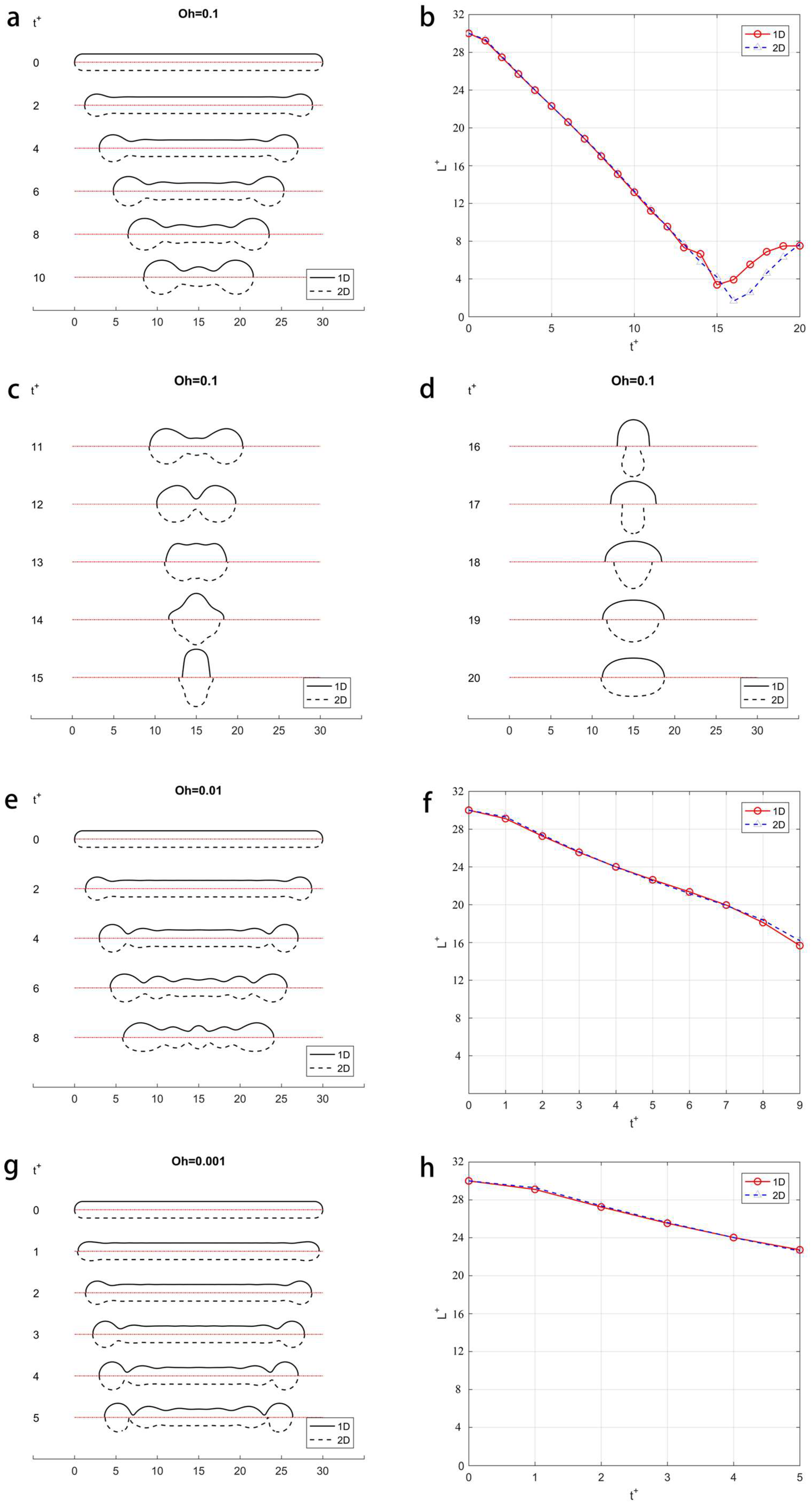
Figure 11.
A typical step driving pressure.
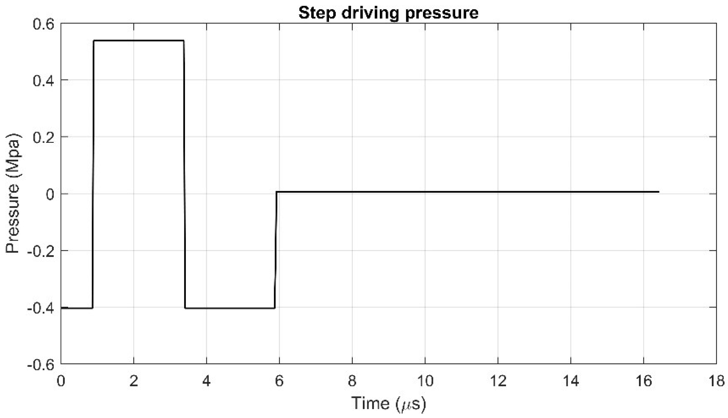
Figure 12.
Single droplet ejection in DOD inkjet under a typical step driving pressure.

Figure 13.
Comparison between 1D and 2D methods: (a) Accumulative liquid volume from the orifice plane; (b) Mean velocity.
Figure 13.
Comparison between 1D and 2D methods: (a) Accumulative liquid volume from the orifice plane; (b) Mean velocity.

Figure 14.
Two typical PIJ driving pressure waveforms.
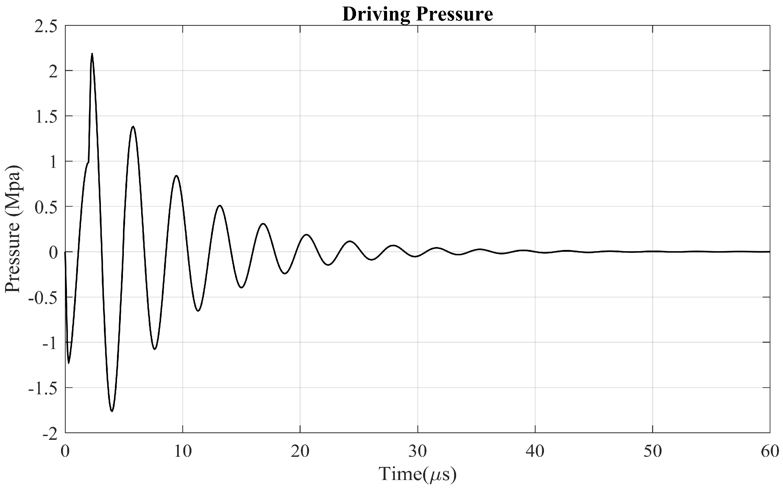
Figure 15.
Droplet ejection with (a) Oh = 0.01; (b) Oh = 0.05; (c) Oh = 0.1.
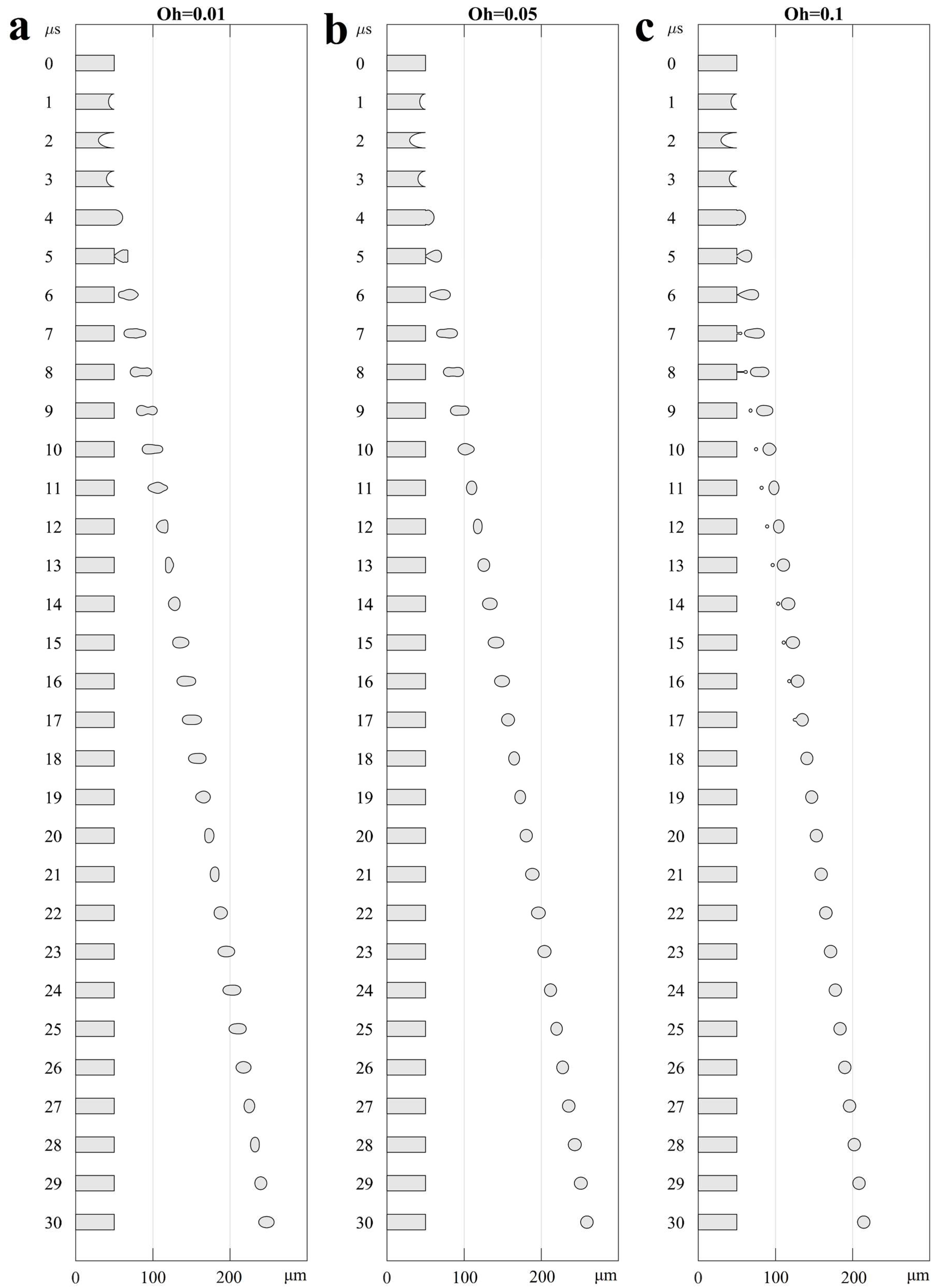
Figure 16.
Comparison of accumulative volume from three ejection.

Table 1.
Comparison of scaled breakup times from our 1D simulation (third row) with Ashgriz’s (first row) 2D simulation and Furlani’s 1D simulation (second row).
Table 1.
Comparison of scaled breakup times from our 1D simulation (third row) with Ashgriz’s (first row) 2D simulation and Furlani’s 1D simulation (second row).
| ε = 0.05 | ||||
|---|---|---|---|---|
| k+ = 0.2 | k+ = 0.45 | k+ = 0.7 | k+ = 0.9 | |
| Re = 200 | 25.213 | 12.911 | 10.035 | 14.495 |
| 25.0 | 12.6 | 9.7 | 11.0 | |
| 25.036 | 12.722 | 9.767 | 11.098 | |
| Re = 10 | 26.683 | 14.299 | 11.623 | 14.83 |
| 27.9 | 14.3 | 11.4 | 14.4 | |
| 27.005 | 14.306 | 11.480 | 14.523 | |
| Re = 0.1 | 230.6 | 243.2 | 311.9 | 628.2 |
| 227 | 238 | 305 | 634 | |
| 234.025 | 245.748 | 313.740 | 642.686 | |
Table 2.
A typical step driving pressure.
| 0.00–0.21 | −60 |
| 0.21–0.82 | +80 |
| 0.82–1.43 | +60 |
| 1.43– | +1 |
© 2018 by the authors. Licensee MDPI, Basel, Switzerland. This article is an open access article distributed under the terms and conditions of the Creative Commons Attribution (CC BY) license (http://creativecommons.org/licenses/by/4.0/).
Share and Cite
MDPI and ACS Style
Jiang, H.; Tan, H. One Dimensional Model for Droplet Ejection Process in Inkjet Devices. Fluids 2018, 3, 28. https://doi.org/10.3390/fluids3020028
AMA Style
Jiang H, Tan H. One Dimensional Model for Droplet Ejection Process in Inkjet Devices. Fluids. 2018; 3(2):28. https://doi.org/10.3390/fluids3020028
Chicago/Turabian StyleJiang, Huicong, and Hua Tan. 2018. "One Dimensional Model for Droplet Ejection Process in Inkjet Devices" Fluids 3, no. 2: 28. https://doi.org/10.3390/fluids3020028