Material Transport under a Wave Train in Interaction with Constant Wind: A Eulerian RANS Approach Combined with a Lagrangian Particle Dispersion Model

Abstract

The interaction of a developed train of gravity deep water waves with suddenly applied winds is investigated in this manuscript. The direction of the wind is the same as that of the wave train (i.e., following) and its imposed surface shear stress is constant and steady. The focus of this study is on a micro-scale water wave field where the time scale is on the order of ten wave periods and the length scale is on the order of ten wave lengths. Accurate 2D Reynolds-averaged Navier–Stokes (RANS) multi-phase simulations of Navier–Stokes equations are performed in a Eulerian framework to capture the flow features, induced by the wave field and the surface wind. The sufficiently large spatial domain in the horizontal direction, combined with the sufficiently long simulation time, permits the development of surface currents and the consequent formation of a near-surface shear layer. The interaction of surface currents with the wave orbital velocity field results in the generation of spilling breaking waves. Downstream of the domain, vertical turbulent structures are observed as the result of such breaking waves. Lagrangian particle tracking is performed, using the RANS simulation velocity and eddy diffusivity data. A second order random acceleration particle tracking method is applied with the vitally important spatial gradients of the eddy diffusivity (Journal of Marine Science and Engineering, 2018, 6, 10.3390/jmse6010007.) also included in calculations. The spatial gradients of the eddy diffusivity were proved to be a key factor in material transport simulations. Our particle tracking results exhibit strong vertical mixing downstream of the domain and by means of visualizing the spiral trajectory of neutrally buoyant particles. Such enhanced vertical mixing (caused by horizontal winds) is the result of the strong near-surface advection (induced by currents) and the turbulence (induced by breaking waves). The objectives of this paper are twofold. Firstly, a numerical approach to simulate wind breaking waves is proposed based on: using $K-ϵ$ RANS model to capture turbulence features, employing the Volume of Fluid Method (VOF) to model the free surface flow, and applying a constant shear stress body force at the interfacial cells to simulate the wind force. Such treatment of the winds eliminates the need for fully resolving the air phase. The computed eddy viscosity profiles are in good agreement with the experimental profiles reported in the literature (${\nu }_t=-\kappa u^{*}z$, Journal of Physical Oceanography, 1977, 7, pp. 248–255; Journal of Physical Oceanography, 1984, 14, pp. 855–863). Secondly, effects of the horizontally applied wind on the vertical mixing and eddy viscosity profiles on the water column are studied. It is observed that, away from the surface and outside the shear layer, the negative horizontal gradient of eddy diffusivity (induced by the dampening effect of breaking surface waves), combined with the downwards advection velocities (induced by breaking waves), results in an enhanced vertical mixing and reduced horizontal drift of transported material.

1. Introduction

The interaction of surface gravity waves and surface winds results in some of the most important oceanographic processes such as: breaking waves, material transport and vertical mixing, Langmuir cells, momentum and scalar transfer at the air–sea interface and coastal upwelling [1,2,3]. Strong winds generate shear layers in the upper mixing layer, which interact with the wave orbital velocity field [4,5]. In shallow waters, where the orbital wave velocities are strong enough to affect the bottom shear layer, the bottom boundary can be affected by strong surface wind. There is a wealth of knowledge, gained by field measurements, laboratory experiments, or numerical simulations, about the effects of the wind induced surface shear current on the bottom boundary layer in shallow waters. In a broader context, the theory of near-surface response of wave fields to wind currents is quite well developed with the key feature being reported as the vertical variations of eddy viscosity. The earliest of such studies in the literature is the classical wind-driven currents by Eckman [6] in which the eddy viscosity was assumed constant across the entire vertical column. Thomas [7] proposed a more realistic model for eddy viscosity: ${\nu }_t=-\kappa u_b^{*}{z}_b$ where $\kappa$ is von Kármán’s constant and $u_b^{*}$ is the bottom surface friction velocity, given by $u_b^{*}={({\tau }_b/\rho )}^{1/2}$, where ${\tau }_b$ is bottom shear stress and $\rho$ is water density. Madsen [8] proposed a modified equation for eddy viscosity, which was based on the surface friction velocity $u_s^{*}$ given by ${\nu }_t=\kappa u_s^{*}(h-z_b)$, where h is the water depth. The model was based on the assumption that eddy viscosity increases linearly with the depth. Using acoustic bubble measurements, Thorpe [9] reported that eddy viscosity profile is of the form proposed by [8], except for a near-surface zone, where it is directly affected by breaking waves. Such near-surface behavior will later shown to be the case in this manuscript.

As far as the vertical material or properties transport in such flows are concerned, eddy viscosity was shown [10,11] to greatly affect the transport phenomenon and was reported as the key feature in such wave and wind interactions. Extensive studies have dealt with the problem of deep water wave and wind interactions [4,12,13]; however, the problem of air–sea interaction continues to be a key unresolved issue for over half a century [14]. This is particularly true in regard to the numerical simulation studies and given the two-stage, unsteady, and abrupt characteristics of the breaking phenomena. In an ideal setup and to fully represent the resulting breaking waves, the air phase must be fully resolved prior to being imposed on a train of waves. To eliminate such an expensive requirement, a new numerical method is proposed here. Such a method is based on applying the wind shear stress as a body force at the air–water interface.

Although recent studies have been successfully implementing Direct Numerical Simulation (DNS) to deep water breaking waves in the absence of winds [3,15,16,17], there are very few DNS or Large Eddy Simulation (LES) studies in which wind breaking waves in deep water are simulated [18,19]. Some studies model air flows over idealized waves [20,21], while others perform very accurate Direct Numerical Simulations over very small domains and short periods [22]. Pizzo et al. [15], as the closet example to this current work, studied the Lagrangian drift of particles under dispersive focusing breaking waves (with no winds involved), using their accurate DNS data. The present study, on the contrary, uses the less accurate RANS method to model a more realistic wave flow situation and without the irrotational flow assumption. To assess the material transport in this work, Lagrangian particle tracking is performed on the previously resolved RANS data. Given their simplicity, Lagrangian approaches are very suitable for studying geophysical and environmental processes such as: material transport in oceans [23,24], fate of air pollutant particles [25], and oil slick movement during oil spills [26]. However, the effect of transport induced by smaller turbulent scales should be properly implemented when applying Lagrangian particle tracking methods. Otherwise, inaccurate results could be obtained, as was reported in [27,28], where the effect of the inclusion of the gradient of diffusivity in the Random Walk Method was studied. It was demonstrated [27,28] that, by not including the gradient of diffusivity in the calculation, particles accumulate in the areas with lower diffusivity. This problem should be handled by direct calculation of the spatial gradients of eddy diffusivity tensor components and its inclusion in the random process [29,30,31,32]. It is shown here that the negative horizontal gradient of eddy diffusivity, induced by the damping effect of the breaking waves, is the key factor in the enhanced vertical mixing under wind breaking waves. This study is the continuation of our previous work [27] where the effect of non-breaking waves on oil droplet transport was studied.

2. Governing Equations and Problem Setup

2.1. Eulerian RANS Framework

For an unsteady, viscous, incompressible, two-dimensional flow, the Reynolds averaged Navier-Stokes equations are given as:

$$\frac{\partial \rho u_j}{\partial x_j}=0,$$

(1)

$$\frac{\partial \rho u_i}{\partial t}+u_j\frac{\partial \rho u_i}{\partial x_j}=-\frac{\partial P}{\partial x_i}+\frac{\partial }{\partial x_j}[(\mu +{\mu }_t)\frac{\partial u_j}{\partial x_j}]+f_i,$$

(2)

$$\frac{\partial \rho K}{\partial t}+\frac{\partial \rho K{u}_j}{\partial x_j}=\frac{\partial }{\partial x_j}[{\alpha }_k(\mu +{\mu }_t)\frac{\partial K}{\partial x_j}]+P_k-\rho ϵ,$$

(3)

$$\frac{\partial \rho ϵ}{\partial t}+\frac{\partial \rho ϵu_j}{\partial x_j}=\frac{\partial }{\partial x_j}[{\alpha }_{ϵ}(\mu +{\mu }_t)\frac{\partial ϵ}{\partial x_j}]+C_{1ϵ}\frac{ϵ}{K}{P}_K-C_{2ϵ}\rho \frac{{ϵ}^2}{K}-R_{ϵ},$$

(4)

where Equations (1) and (2) represent the conservation of mass and conservation of momentum in two spatial directions, respectively. Equations (3) and (4) represent the turbulence k-epsilon model consisting of a transport equation for turbulent kinetic energy (TKE) (Equation (3)) and a transport equation for TKE dissipation (Equation (4)) [33]. In the equations above, $i=1,2$ with index 1 corresponding to streamwise and 2 to wall-normal directions, respectively. A repeated index indicates summation over the index. Here, t is time, $u_i$ is the Reynolds-averaged fluid velocity vector, P is the Reynolds-averaged pressure, $f_i$ is the body force term, $\rho$ is constant density of the fluid, $\mu$ is dynamic viscosity, K is TKE, $ϵ$ is TKE dissipation rate, $P_k$ is TKE production rate due to the mean velocity shear, ${\alpha }_k$ and ${\alpha }_{ϵ}$ are the inverse Prandtl numbers for K and $ϵ$, respectively, $C_{1ϵ}=1.42$ and $C_{2ϵ}=1.68$ are model constants, and ${\mu }_t$ is eddy viscosity. Note that the eddy viscosity tensor is taken to be diagonal with equal diagonal entries, thus we consider an isotropic eddy diffusivity. The $K-ϵ$ model’s isotropic eddy viscosity is given by

$${\mu }_t=\rho C_{\mu }\frac{K^2}{ϵ},$$

(5)

with $C_{\mu }=0.0845$. The last term on the right-hand side of Equation (4) is specific to the Re-Normalisation Group (RNG) $K-ϵ$ model [34] and is given as

$$R_{ϵ}=\frac{C_{\mu }\rho {\eta }^3(1-\eta {\eta }_0)}{1+\beta {\eta }^3}\frac{{ϵ}^2}{K},$$

(6)

with $\eta \equiv SKϵ$ with ${\eta }_0=4.38$ and $\beta =0.012$ being model constants. Note that $S={(2S_{ij}{S}_{ji})}^{1/2}$ with $S_{i,j}=\frac{1}{2}(\frac{\partial u_i}{\partial x_j}+\frac{\partial u_j}{\partial x_i})$. To model the multi-phase free-surface flow, the Volume Of Fluid (VOF) method is used. The two-phase fluid is composed of air and water. The governing equations (described above) for both of the phases are the same. However, the density, dynamic viscosity, and eddy viscosity depend on the phase in the local cell and may vary between adjacent cells. At each cell, the dynamic viscosity and density are calculated by:

$$\begin{array}{c}\hfill \rho ={\alpha }_w{\rho }_w+(1-{\alpha }_w){\rho }_a,\\ \hfill \mu ={\alpha }_w{\mu }_w+(1-{\alpha }_w){\mu }_a,\end{array}$$

(7)

where ${\alpha }_w$ is a scalar value representing volume fraction of water with value of 1 corresponding to a full water cell and 0 corresponding to an air cell. An extra transport equation for ${\alpha }_w$ is solved to track the interface during the simulation [35].

2.2. Lagrangian Particle Dispersion Framework

The governing advection diffusion in a Eulerian framework [36] can be written as

$$\frac{\partial C}{\partial t}+(u_j)\frac{\partial C}{\partial x_j}=\frac{\partial }{\partial x_j}(D_j\frac{\partial C}{\partial x_j}),$$

(8)

where C is the Reynolds-averaged tracer concentration (e.g., oil with C being oil mass per unit volume of water), $D_i$ is the turbulent eddy diffusivity in the corresponding directions and, given the difficulties associated with numerical solutions of highly advective flows [37], the solution of Equation (8) can require artificial numerical diffusion leading to inaccurate concentration solutions. By the passive tracers assumption (i.e., the oil particle motion has no effect on the dynamics of the carrier fluid phase), the oil is treated as a discrete phase that is only dispersed and diffused by the flow. Such flow induced particle advection and diffusion are studied using the Random Walk Method. The method consists of time integration of the Lagrangian velocity and acceleration equations for individual particles (i.e., Random acceleration method). To track a particle located at the position $x_i^{(n)}$ and at the starting time $t^{(n)}$, the location at the time $t^{(n)}+\Delta t$ is found by the following pair of stochastic equations [38] needing to be solved:

$$u_p^{(n)}=u_p^{(n-1)}+F_D(u_i^{(n-1)}-u_p^{(n-1)})\Delta t+(\frac{g({\rho }_p-\rho )}{{\rho }_p})\Delta t,$$

(9)

$$x_i^{(n+1)}=x_i^{(n)}+u_p^{(n)}\Delta t+\frac{\partial D_i}{\partial x_i}\Delta t+R\sqrt{2D_i\Delta t},$$

(10)

where R is a random Gaussian distribution. The second term on the right-hand side of Equation (10) represents the advection induced by the carrier velocity field. The third term is the divergence of the eddy diffusivity whose significance will be discussed later in the manuscript. The last term is a stochastic model representing the fluctuating turbulent field constructed from the RANS simulation data. Using the Boussinesq hypothesis and assuming that the eddy diffusivity is isotropic [33,39,40], we drop its index and model the eddy diffusion coefficient as

$$D=\nu +{\nu }_t\approx {\nu }_t=C_{\mu }\frac{K^2}{ϵ},$$

(11)

with $\nu =\mu /\rho$ being the kinematic viscosity of fluid. Note that for a high Reynolds number flow, the eddy viscosity is orders of magnitude larger than dynamic viscosity and hence the latter could be neglected.

Furthermore, in (9), $u_p$ and ${\rho }_p$ are particles velocity and density and the drag force acting on the particle by the surrounding fluid id simulated by $F_D(u_i-u_p)$ given by:

$$F_D=\frac{18\mu }{{\rho }_p{d}_p^2}\frac{C_D{R}_e}{24},$$

(12)

where $d_p$ is particles diameter, $C_D$ the drag coefficient for spherical objects, and $R_e$ the relative Reynolds number, defined as $R_e=\rho d_p|u_i-u_p|/\mu$.

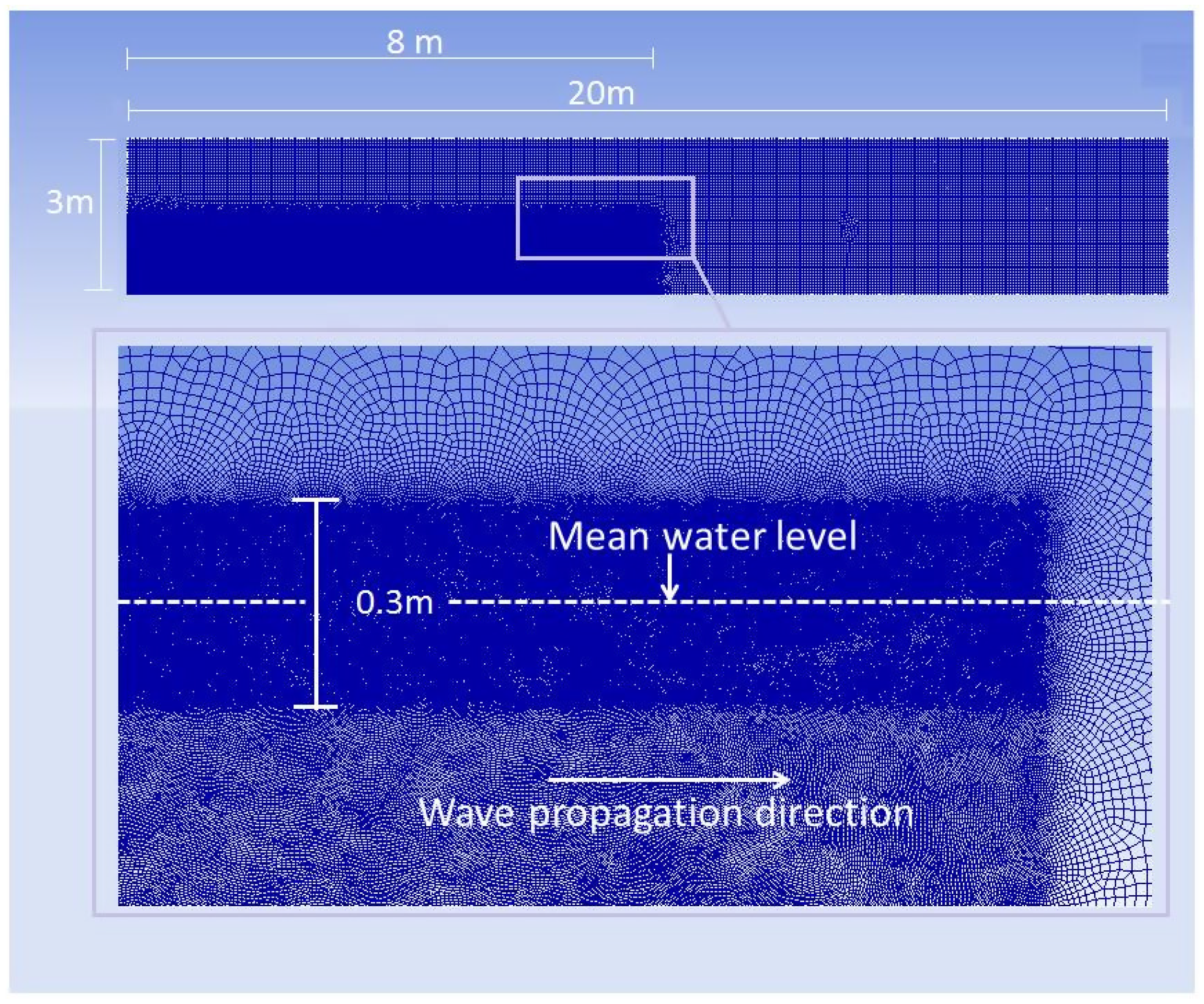
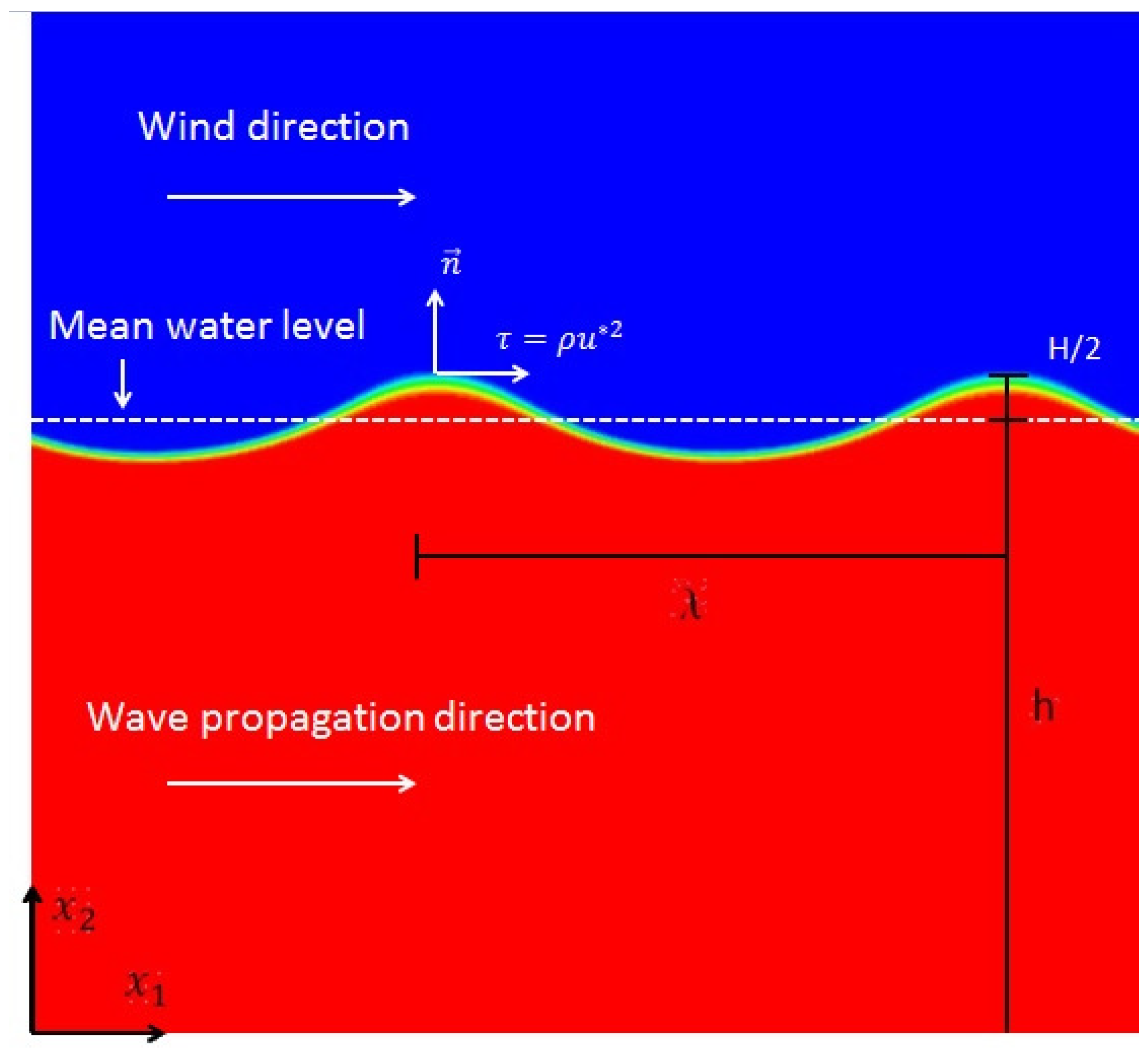
2.3. Flow Configuration

The domain of simulation consists of a rectangular box of 20 m × 3 m in $x_1$ and $x_2$ directions, respectively (see Figure 1). A mesh comprising 835,229 nodes and 834,239 mixed quadrilateral cells was used for the simulation. Given the sensitivity of the VOF method to coarse meshes near the interface area, the mesh was refined significantly near the free surface. The refinement was performed within a rectangular region. The size of the rectangular region was 8 × 0.3 m in the $x_1$ and $x_2$ directions, respectively, with the middle of the region corresponding to the mean water level. Within this rectangular region, the mesh size varied between 0.001 m and 0.005 m. Outside of this region, the mesh size varied between 0.001 m and 0.01 m. Flow simulations were performed using the commercial package ANSYS FLUENT (ANSYS${}^{\circledR }$ Academic Research, Release 15, Canonsburg, PA, USA) [35].

The numerical discretization was based on the Finite Volume Method employing the VOF technique to capture the air–water interface and the RNG $K-ϵ$ turbulence model. The Finite Volume Method was used with second-order upwind schemes to discretize the equations in space. The implicit and first order SIMPLE method is employed for the time discretization, given its stability and fast convergence [35]. The particularly small chosen time step of $0.0005s$ to capture the unsteadiness of the flow [41] and to fulfill the CFL number conditions and restrictions. The solution was started from the rest and with an initial water level equal to h. At the input boundary (the left edge in Figure 1), a Dirichlet velocity boundary condition is imposed. The velocity value at the input boundary is calculated using Equation (14). Standard wall models are applied at the right and bottom edges of the rectangular domain, while the pressure outlet boundary condition is applied on the top edge.

2.3.1. Wave Formulation

The simulation was started initially with the modeling of non-breaking deep water waves. The setup is depicted in Figure 2 with the characteristic wave length $\lambda$ being the horizontal distance between the crests (or troughs), wave height H is the vertical distance between the crest and trough of the wave, and the wave period is T. The wave number is defined as $k=2\pi /\lambda$ and the angular frequency is given by $\sigma =2\pi /T$. For deep water waves, the wave length is linked to the frequency using the dispersion relation [42] as

$$\sigma =\sqrt{kg},$$

(13)

where g is acceleration due to gravity. The analytical solution for velocities using the first order linear wave theory is given as

$$\begin{array}{c}{u}_i(x_1,x_2,t)=\hfill \\ {\delta }_{1,i}\left(\frac{kgH}{2\sigma }\frac{cosh(k{x}_2)}{cosh(kh)}cos(k{x}_1-\sigma t)+\frac{3H^2\sigma k}{16}\frac{cosh(2k{x}_2)}{sin{h}^4(kh)}cos2(k{x}_1-\sigma t)\right)+\hfill \\ {\delta }_{2,i}\left(\frac{kgH}{2\sigma }\frac{sinh(k{x}_2)}{cosh(kh)}sin(k{x}_1-\sigma t)+\frac{3H^2\sigma k}{16}\frac{sinh(2k{x}_2)}{sin{h}^4(kh)}sin2(k{x}_1-\sigma t)\right),\hfill \end{array}$$

(14)

where h is the mean water depth. The chosen wave for simulation has a period of $T=1s$ and a height of $H=0.15$ m. The wave length calculated by the dispersion relation in (13) is equal to $\lambda =1.56$ m. To ensure a deep water wave condition, the mean water depth was set equal to $h=1.2$ m. Furthermore, water density was taken as 998.2 kg/m${}^3$, air density as 1.225 kg/m${}^3$, water dynamic viscosity as 1.003 × 10${}^{-3}$ kg/ms, and air dynamic viscosity as 1.7894 × 10${}^{-5}$ kg/m^−s.

2.3.2. Wind–Wave Interaction Simulation

The constant wind that blows in the positive $x_1$ direction is simulated by adding a volume body force to the momentum Equation (2) as given by the following equation:

$$f_i=u^{\ast 2}\frac{\rho \overline{\kappa }}{({\rho }_a+{\rho }_w)/2}\frac{\partial {\alpha }_w}{\partial x_i},$$

(15)

where $\overline{\kappa }$ is the gradient of the normal vector at the interface, $\rho$ is the cell density given by Equation (7) and $u^{*}$ is the friction velocity based on the surface shear stress. To assess the response of near-surface current profile to the wind strength and also to study the resulting vertical mixing, two different cases with different winds are simulated. For the weaker wind, the surface body force is 0.5 [N/m] and, for the stronger wind, the surface body force is 0.6 [N/m]. Friction Reynolds number can be calculated by $R{e}_{\tau }=u^{*}\delta /\nu$ with an average friction velocity for each wind case calculated using Equation (15) and $\delta$ the turbulent length scale. Choosing the shear layer thickness (≈0.1 as shall be seen) as the turbulent length scale, our calculated Reynolds numbers for each wind case are 2280 and 2500 for the developed flow.

2.3.3. Particle Tracking

After simulating the flow, the results were imported into a particle tracking code. The imported results included velocity components, eddy viscosity or diffusivity and water volume fraction ${\alpha }_w$. The code is capable of constructing a triangular unstructured mesh over any set of points and using linear interpolation to calculate the in-between values of the variables. The particle search algorithm locates the particle and links it to the corresponding triangle in which the particle has traveled to. Moreover, the transient input data are updated at each tracking time step. Using an unstructured linear mesh provides the capability of constructing the spatial gradients of eddy diffusivity. Often overlooked, the gradient of eddy diffusivity is particularly important in mass transport studies and must not be neglected [27,28]. Particle tracking in general can be performed for light and buoyant (e.g., oil droplets, bubbles) or denser and submerging (e.g., sediment ) particles. To avoid the complication brought about with buoyancy and inertia effects, given that the main goal is to compare two cases with different wind strengths, we choose to conduct the experiment on a group of 1000 of neutrally buoyant particles. Furthermore, the tracking was performed over a 10 wave period time span after the wind was activated. The particles were uniformly distributed and seeded at two different streamwise locations; the first particle group was distributed in the spatial domain of $x_1\in [4.5,5]$ m and the fixed elevation of $x_2=1.15$ m, while the second group occupied the spatial span of $x_1\in [5.5,6]$ m while sharing the same vertical location with the first group.

3. Results

3.1. Numerical Simulation Validation

The solution procedure in this study comprises the application of a sudden constant following wind on a developed regular wave train. The simulation of the regular wave was started from the rest. The simulation was continued until a fully developed flow was attained. To collect the essential data to perform the test particle tracking, the simulation was continued for another 10 wave periods. These numerical results were compared with the analytical solutions, obtained by the linear wave theory [42]. Our previous paper [27] showed the validity of the simulations and therefore such results are not repeated here. To simulate wind breaking waves, the wind body force was added on and the simulation is conducted for another 10 wave periods. Note that, as two different winds scenarios are simulated, two different simulations are conducted with the same initial conditions and different wind body forces.

3.1.1. Non-Breaking Wave Simulation

In our previous work [27], the validity of non-breaking wave simulations were demonstrated by providing the plots for: comparison of the time series of velocity components with the analytical solution from second order linear wave theory, and the comparison of vertical profiles of velocity components with their analytical profiles. Furthermore, the calculated averaged Stokes drift velocity (based on the particle tracking results) showed good agreement with the theoretical value (based on Stokes drift theory). To present the following results, the wind force was applied to the previous non-breaking wave simulations results.

3.1.2. Wind–Wave Simulation

As was mentioned earlier, the following wind was suddenly applied to a train of developed deep water waves. The interaction of the surface winds and the orbital velocity of waves results in small spilling breaking waves as shown in Figure 3. By choosing the characteristic wave slope $S=ak$, our calculated initial wave slope is $0.302$. As the result of wind-induced surface current, the wave steepens slightly until the crest becomes unstable. The slight increase of the steepness, however, is not significant enough to push the breaking wave type into the more extreme plunging or collapsing scenarios. Based on our observations, the fourth wave in the train exhibits the most severe cases of breaking and the fifth wave suffers height loss and energy dissipation (which results in its flattening). This is figuratively consistent with the observations of [17], where the total dissipation of the wave in the first four periods were reported (although the breaking wave generation mechanism in that study was completely different and was based on the Dispersive Focusing Method). The dissipation of the fifth wave is evident in Figure 3. The figure illustrates the water volume fraction ${\alpha }_w$ at the time $t=7[s]$ after the winds were started. The plot is zoomed in at the horizontal span of $x_1\in [6,7.6]$ m (where the fifth wave is located and also where an enhanced vertical mixing will be observed in Figure 4). Furthermore, velocity vectors are superposed to the contours in order to illustrate the relative strength of advective currents for each wind case. The figure illustrates formation of the surface currents which are stronger near the crest ($x_1\in [7,7.6]$ m, $x_2\in [1.1,1.3]$ m) and with higher magnitude for the stronger wind (bottom panel). Furthermore, this figure shows an area with strong downward vertical velocity vectors ($x_1\in [6.6,6.9]$ m, $x_2\in [0.9,1.3]$ m). The downward velocity magnitude is higher for the case with weaker wind. The lower velocity magnitude for the case with stronger wind can be related to the stronger near-surface current that affects the vectors by means of energy dissipation. Moreover, the breaking occurs as the result of the collision of upwards orbital velocities, induced by the waves, and the positive horizontal current flow, induced by the wind. The aforementioned collision phenomenon is evident in the area $x_1\in [7.4,7.6]$ m, $x_2\in [1.2,1.3]$ m. Given the stronger near-surface current for the case with stronger wind, stronger breakers are observed for this case.

Figure 5 shows the wave-length and time averaged profiles of wall-normal eddy viscosity. Time averaging is performed over time span of the last three wave periods and wave-length averaging is performed over the third (occupying the streamwise span of $x_1\in [3.5,5]$) and the fourth (occupying the streamwise span of $x_1\in [5,6.5]$) waves in the train. The plot corresponds to both of the cases with weaker (solid and dotted blue lines) and stronger (solid and dotted red lines) winds as well as the cases with no wind (regular waves). To demonstrate that the observed dissipation is indeed a direct result of wind–wave interactions and not a numerical induced dissipation, the profiles of eddy viscosity corresponding to both the third and fourth waves for the case with no wind are also included (solid and dotted green lines).

Based on Figure 5, downstream of the domain where the turbulence is developed, the wall-normal profiles of time averaged eddy viscosity show close agreement with Madson’s relation [8] and for both the wind cases. Based on Madson’s relation [8], the eddy viscosity is assumed to be proportional to the depth

$$\nu =-\kappa u^{*}\widehat{x_2},$$

(16)

where $\kappa$ is von Kármán’s constant (≈0.4) and $\widehat{x_2}$ is the vertical component of a coordinate system which originates at the free surface and is positive downwards. By transforming such vertical coordinate to our chosen Cartesian system (which origins at the bottom wall and is positive upwards), we can write: $\widehat{x_2}=(\eta +h)-x_2$. Note that $\eta$ is the free surface elevation measured from the mean water level. As the eddy viscosity profile is presented in a time averaged manner, it is fair to assume that the averaged value of $<\eta {>}_{x_1,t}$ should be approximately equal to 0. Given this, the averaged profiles should start at the vertical axis at $x_2=h-\widehat{\zeta }$ where $\widehat{\zeta }$ is the thickness of the shear layer, the layer which is directly affected by breaking waves. Using acoustic bubble measurements, Thorpe [9] showed that eddy viscosity profile is of the form (16), except for a near-surface zone where the flow is directly affected by breaking waves, with the estimated thickness of this zone $\widehat{\zeta }$ to be approximately 10 times the $(g/{\sigma }^2)H$ value. Given our simulated wave data, the calculated shear layer thickness, $\widehat{\zeta }$ is $0.2236[m]$, which is based on the location where the eddy viscosity reaches its maximum value and its vertical gradient changes sign. This value matches the “medium profile” of Jenkins [43] ($\widehat{\zeta }=6(g/{\sigma }^2)H$). For the matching profiles (downstream and shown in solid red and blue lines) in Figure 5, the calculated shear layer thickness is approximately the same as the theoretical value. For illustration purposes and to show the slope match, we had to slightly shift the profiles in Figure 5. Furthermore, the gradual decrease of eddy viscosity value in streamwise $x_1$ direction is the direct result of the dissipation induced by the breaking waves. Such drastic decline in eddy viscosity values produces a negative horizontal gradient of eddy diffusivity, which, as will be shown, causes enhanced mixing and greatly affects material transport. Downstream of the domain ($x_1=7$ [m]), the eddy viscosity reaches the equilibrium value (solid red line) and hence matches a theoretical value given by (16).

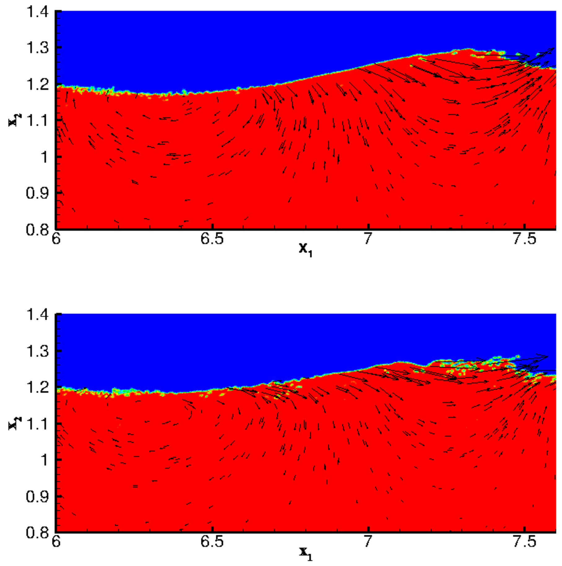
3.2. Drift Current Formation

Our results attest to the formation and further development of near-surface drift currents as the direct result of applied winds. Figure 6 presents the instantaneous snapshots of streamwise velocity component ($u_1$ [m/s]) at $t=5$ [s] (left-hand side panels) $t=10$ [s] (right-hand side panels). The top panels correspond to the case with the weaker wind and bottom panels correspond to the case with the stronger wind. To illustrate details of the surface current, the plot is zoomed in a domain of $x_1\in [5,6.5]$ m and $x_2\in [0.8,1.4]$ m. As it can be seen, the evolution of drift currents in time results in the negative velocity areas ($x_1\in [6,6.5]$ m, $x_2\in [0.8,1]$ m) shrinking and the velocity magnitudes decreasing. On the other hand, the positive velocity areas ($x_1\in [5,6.5]$ m, $x_2\in [1,1.2]$ m) start to grow and the velocity magnitudes start to increase. The effect is more pronounced for the case with the stronger wind (bottom panels). Furthermore, by comparing the wave heights between the cases with different winds, it can be concluded that the stronger wind blows the waves flat [44].

Figure 7 presents the instantaneous snapshots of wall-normal velocity component ($u_2$ m/s) at $t=5$ [s] (left-hand side panels) $t=10$ [s] (right-hand side panels). The top panels correspond to the case with the weaker wind and bottom panels correspond to the case with the stronger wind. To illustrate more details, the plot is zoomed in on a horizontal domain of $x_1\in [5,6.5]$ m. As it can be seen, the formation of the drift currents results in generations of narrow streaks of negative vertical velocity ($x_1\in [5.4,5.8]$ m, $x_2\in [1,1.2]$ m). Details of the vertical structures are shown in Figure 8.

To assess the drift current velocity, Figure 9 is presented. The figure shows the horizontal structure of the drift currents during a wave period and in three streamwise locations. Based on this figure, upstream of the domain (the top panel corresponding to $x_1=3$ [m]), the surface current has the maximum local velocity (approximately 1 [m/s] for the weaker wind and 1.2 [m/s] for the stronger wind). Towards downstream, the streamwise velocities at the surface start to decrease (as the result of breaking waves and the ensuing dissipation) and the negative wall-normal velocity components start to increase. Note that the high local values at the interface are the result of lower density at the interface and hence the average current velocity should be calculated by integrating the local values in wall normal direction and only after filtering the wave velocity. Finally, the observed high horizontal velocities at the surface greatly affect the light material that can float on water surface (e.g., oil) and greatly increase their drift motion, as was shown in [15] where added drifts as large as 10 times the Stokes drift were reported for the particles at the surface. As it will be seen in the upcoming section, our particle tracking experiments take place deeper in the water column and the particles therefore are seeded and tracked outside the surface shear layer. The primary focus in our studies is on the vertical mixing and to demonstrate the drastically different effect of turbulence on the material transport in such regions.

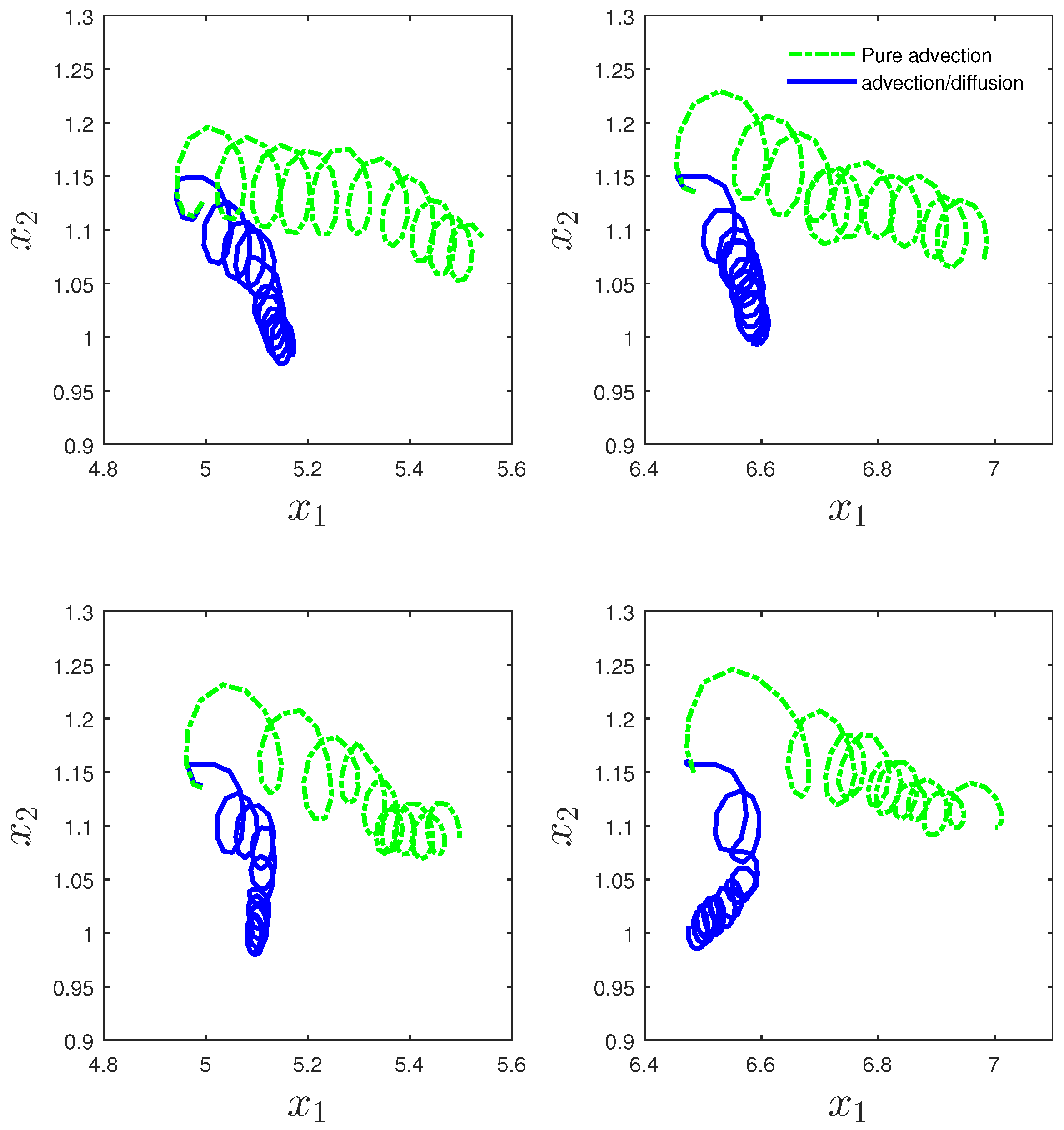
3.3. Particle Tracking and Vertical Mixing

In this section, Lagrangian ensemble-averaged particle trajectories are presented in order to better understand the combined effect of advective velocities (induced by the breaking wave motion) and the diffusion (induced by turbulence). Results are obtained by tracking 1000 individual neutrally buoyant particles and calculating the plume trajectory by averaging the trajectories over all of the particles. The chosen number of particles was sufficiently large to ensure that the results are not affected by a further increase of the number of particles. Figure 4 presents the ensemble averaged trajectories for particles released at two different streamwise locations, $x_1\in [4.5,5]$ m, $x_1\in [6.5,7]$ m while all the particle sets had the identical wall-normal location of $x_2=1.15$ m. The chosen location is outside the surface shear layer as was observed in Figure 5. As was mentioned, the primary focus is on the vertical mixing. The dashed-dotted lines in the graphs correspond to the trajectories due to the pure advection and their values are calculated by setting eddy diffusivity and its gradients equal to 0 (i.e., the last two terms in the right-hand side of Equation (10)). Comparing the wind–wave induced particle trajectories in Figure 4 with the classical wave induced drift motion trajectories spirals, one realizes that the horizontally blown wind induces enhanced vertical mixing. Such mixing is induced through the downward strong advection in areas where wave breaking occurs (upstream of the domain) and through the strong turbulence diffusion prior to breaking (downstream of the domain). Downstream of the domain the turbulence diffusion is not affected by the breaking waves. Thereby a thicker near-surface shear layer is formed. Such layer contains higher eddy viscosity/diffusivity values (evident in Figure 5, blue lines). Comparing the particle trajectories in upstream (left top and bottom panels) and downstream (right top and bottom panels) of the domain, one realizes that in the upstream region both the drift motion and vertical mixing affect the trajectories. Downstream of the domain, however, vertical mixing is the dominating force that results in enhanced mixing and negative drift motion for the stronger wind case (bottom right panel). For the case with the stronger wind, sudden drops in trajectories are associated with the stronger breakers on the surface. As a result of wind breaking waves, turbulent diffusion plays a more significant role in the material transport. This is evident in all the bottom panels of Figure 4 where there are clear different trends of particle movements when the cases with pure advection (green lines) are compared with the cases with advection/diffusion (blue lines). To better understand the effect of turbulence diffusion, we next present the averaged wall-normal profile of eddy diffusivity.

Figure 10 presents the vertical profile of streamwise-time averaged eddy diffusivity profiles for the case with wind body force $f=0.5$ [N/M] (blue labeled as “Weaker wind”), the case with the wind body force $f=0.6$ [N/M] (red labeled as “Stronger wind”) and the case with no wind stress and with non-breaking waves. Interestingly, the streamwise-time averaged eddy diffusivity matches a theoretical line similar to that of eddy viscosity reported in ([8]).

The surface shear layer is significantly thinner for the case with pure waves and no wind. The thinner boundary layer results in much sharper gradients of eddy viscosity/diffusivity at the surface. Sharp gradients of the aforementioned quantities result in vertical diffusion mixing near the surface for the case with no wind. However, as it was mentioned before, a combination of two factors results in stronger mixing for the cases with blowing winds—firstly, the strong downward advection downstream of the domain, which is induced by the breaking waves; secondly, the thicker near-surface shear layer with stronger turbulence activities upstream of the domain, observed in Figure 5. The negative drift downstream of the domain for the case with stronger wind (right bottom panel of Figure 4) is to be explained as the result of the combined effect of the weakened downward wave orbital motion and the negative stream-wise gradient of eddy diffusion $\partial D/\partial x_1$ (as the result of wind induced dissipation that is higher upstream) manifesting as a negative streamwise advective velocity.

4. Conclusions

Material transport under the wind breaking waves was investigated. The present study was focused on micro-scale spatial and temporal scales compared to our previous work [27], which focused on material transport under non-breaking waves without the presence of wind. Based on our current results, in the water column and outside the shear layer, mass transport is significantly affected by the wind and through the breaking waves on the surface. A combination of two different mechanisms, namely, the enhanced downwards advection induced by the interaction of the breaking waves with the surface current, and the diffusion that is induced by turbulence, results in enhanced mixing in the water column. A key issue explored in our previous work [27,45,46,47,48] was vertical variations of eddy viscosity and the effect of the inclusion of the gradient of eddy diffusivity in the Random Walk particle dispersion practices. While studying the vertical distribution of particles in the water column induced solely by turbulence diffusion, Visser [28] described the mechanism by which the center of mass of the particles move in the direction of increasing diffusivity. As a result, material is transported from areas of lower eddy diffusivity to areas of higher diffusivity.This mechanism was once again proved to be a very important factor in the material transport studies and therefore should not be overlooked. The results of the current study also agree with our previous findings and confirm the necessity of the inclusion of the gradient of eddy diffusivity in the Random Walk Method. Another important result presented in this paper was the use of the Volume of Fluid method to simulate the wind flow by applying a wind body force in interfacial cells (e.g., Finite Volumes, Finite Elements, etc.) The proposed approach results in a significant decrease in terms of degrees of freedom by eradicating the need to fully model the wind in the air phase. The proposed method led to computation of vertical eddy viscosity profiles, which show good agreement with those from the literature that are based on experimental studies. Our result also manifested the evolution of a surface current, which, by its interaction with the wave motion, results in breaking surface waves. Breaking waves result in the development of an upper mixing layer with the estimated thickness reported in the literature [9,43]. Our calculated thickness shows agreement with those from the literature. To relate the wind stress to the wind velocity for practical applications, given the well-developed theory of response of near-surface current to wind, the appropriate values of surface shear velocity $u^{*}$ could be calculated based on the desired wind speed. Finally, since some of the flow features can not be captured in a 2D simulation, it is vitally important to extend this work to a 3D framework. The proposed method can be used in a 3D framework to study a variety of oceanographic phenomena such as generation of Langmuir cells and wind-induced coastal upwelling. The approach could be applied to shallow water waves to assess the effect of wind on increasing the bottom shear stress and linking it to disruption of the log layer. Turbulence greatly affects material transport; recently, Ghodke et al. [49,50] in their groundbreaking and fully resolved numerical study reported the effects of turbulence on incipient material transport mechanisms. Such high-fidelity simulations can further provide time-accurate eddy viscosity data that otherwise are extremely challenging to obtain using experiments.

References

1. Melville, W.K.; Veron, F.; White, C.J. The velocity field under breaking waves: coherent structures and turbulence. J. Fluid Mech. 2002, 454, 203–233. [Google Scholar] [CrossRef]
2. Peirson, W.L.; Banner, M.L. Aqueous surface layer flows induced by microscale breaking wind waves. J. Fluid Mech. 2003, 479, 1–38. [Google Scholar] [CrossRef]
3. Pizzo, N.E.; Melville, W.K. Vortex generation by deep-water breaking waves. J. Fluid Mech. 2013, 734, 198–218. [Google Scholar] [CrossRef] [Green Version]
4. Grare, L.; Peirson, W.L.; Branger, H.; Walker, J.W.; Giovanangeli, J.P.; Makin, V. Growth and dissipation of wind-forced, deep-water waves. J. Fluid Mech. 2013, 722, 5–50. [Google Scholar] [CrossRef] [Green Version]
5. Sajjadi, S.G.; Thomas, N.H.; Hunt, J.C.R. Wind-over-Wave Couplings: Perspectives and Prospects; Institute of Mathematics and Its Applications: Southend-on-Sea, UK, 1999. [Google Scholar]
6. Ekman, V.W. On the influence of the earth’s rotation on ocean currents. Arkiv för Matematik Astronomi Och Fysik 1950, 2, 1–53. [Google Scholar]
7. Thomas, J.S. A theory of steady wind-driven currents in shallow water with variable eddy viscosity. J. Phys. Oceanogr. 1975, 5, 136–142. [Google Scholar] [CrossRef]
8. Madsen, O.S. A realisitic model of the wind-induced ekman boundary layer. J. Phys. Oceanogr. 1977, 7, 248–255. [Google Scholar] [CrossRef]
9. Thorpe, S.A. On the determination of kv in the near-surface ocean from acoustic measurements of bubbles. J. Phys. Oceanogr. 1984, 14, 855–863. [Google Scholar] [CrossRef]
10. Longuet-Higgins, M.S. Mass transport in water waves. Phil. Trans. R. Soc. Lond. A 1953, 245, 535–581. [Google Scholar] [CrossRef]
11. Longuet-Higgins, M.S. Mass transport in the boundary layer at a free oscillating surface. J. Fluid Mech. 1960, 8, 293–306. [Google Scholar] [CrossRef]
12. Sullivan, P.P.; McWilliams, J.C. Dynamics of winds and currents coupled to surface waves. Annu. Rev. Fluid Mech. 2010, 42, 19–42. [Google Scholar] [CrossRef]
13. Thais, L.; Magnaudet, J. Turbulent structure beneath surface gravity waves sheared by the wind. J. Fluid Mech. 1996, 328, 313–344. [Google Scholar] [CrossRef]
14. Peirson, W.L.; Garcia, A.W. On the wind-induced growth of slow water waves of finite steepness. J. Fluid Mech. 2008, 608, 243–274. [Google Scholar] [CrossRef]
15. Deike, L.; Pizzo, N.; Melville, W.K. Lagrangian transport by breaking surface waves. J. Fluid Mech. 2017, 829, 364–391. [Google Scholar] [CrossRef]
16. Fuster, D.; Agbaglah, G.; Josserand, C.; Popinet, S.; Zaleski, S. Numerical simulation of droplets, bubbles and waves: State of the art. Fluid Dyn. Res. 2009, 41, 065001. [Google Scholar] [CrossRef]
17. Pizzo, N.E.; Deike, L.; Melville, W.K. Current generation by deep-water breaking waves. J. Fluid Mech. 2016, 803, 275–291. [Google Scholar] [CrossRef]
18. Sullivan, P.P.; Edson, J.B.; Hristov, T.; McWilliams, J.C. Large eddy simulations and observations of atmospheric marine boundary layers above non-equilibrium surface waves. J. Atmos. Sci. 2008, 65. [Google Scholar] [CrossRef]
19. Sullivan, P.P.; McWilliams, J.C.; Moeng, C.H. Simulation of turbulent flow over idealized water waves. J. Fluid Mech. 2000, 404, 47–85. [Google Scholar] [CrossRef]
20. Kihara, N.; Hanazaki, H.; Mizuya, T.; Ueda, H. Relationship between airflow at the critical height and momentum transfer to the traveling waves. Phys. Fluids 2007, 19. [Google Scholar] [CrossRef]
21. Shen, L.; Zhang, X.; Yue, D.K.P.; Triantafyllou, M.S. Turbulent flow over a flexible wall undergoing a streamwise travelling wave motion. J. Fluid Mech. 2003, 484, 197–221. [Google Scholar] [CrossRef]
22. Hafsi, A.; Tejada-Martínez, A.E.; Veron, F. Dns of scalar transfer across an air–water interface during inception and growth of langmuir circulation. Comput. Fluids 2017, 158, 49–56. [Google Scholar] [CrossRef]
23. Berloff, P.S.; McWilliams, J.C. Material transport in oceanic gyres. part i: Phenomenology. J. Phys. Oceanogr. 2002, 32, 764–796. [Google Scholar] [CrossRef]
24. Berloff, P.S.; McWilliams, J.C. Material transport in oceanic gyres. part II: Hierarchy of stochastic models. J. Phys. Oceanogr. 2002, 32, 797–830. [Google Scholar] [CrossRef]
25. Wilson, J.D.; Sawford, B.L. Review of lagrangian stochastic models for trajectories in the turbulent atmosphere. Bound.-Lay. Meteorol. 1996, 78, 191–210. [Google Scholar] [CrossRef]
26. Korotenko, K.A.; Mamedovc, R.M.; Kontarb, A.E.; Korotenkob, L.A. Particle tracking method in the approach for prediction of oil slick transport in the sea: modelling oil pollution resulting from river input. J. Mar. Syst. 2004, 48, 159–170. [Google Scholar] [CrossRef]
27. Golshan, R.; Boufadel, M.C.; Rodriguez, V.A.; Geng, X.; Gao, F.; King, T.; Robinson, B.; Tejada-Martínez, A.E. Oil droplet transport under non-breaking waves: An eulerian rans approach combined with a lagrangian particle dispersion model. J. Mar. Sci. Eng. 2018, 6, 7. [Google Scholar] [CrossRef]
28. Visser, W.A. Using random walk models to simulate the vertical distribution of particles in a turbulent water column. Mar. Ecol. Prog. Ser. 1997, 158, 275–281. [Google Scholar] [CrossRef] [Green Version]
29. Dimou, K. 3-D Hybrid Eulerian-LagRangian/Particle Tracking Model For Simulating Mass Transport in Coastal Water Bodies. Ph.D. Thesis, Massachusetts Institute of Technology, Department of Civil and Environmental Engineering, Hong Kong, China, 1992. [Google Scholar]
30. Ermak, D.L.; Nasstrom, J.S. A lagrangian stochastic diffusion method for inhomogeneous turbulence. Atmos. Environ. 2000, 34, 1059–1068. [Google Scholar] [CrossRef]
31. Gouesbet, G.; Berlemont, A. Eulerian and lagrangian approaches for predicting the behaviour of discrete particles in turbulent flows. Prog. Energy Combust. Sci. 1999, 25, 133–159. [Google Scholar] [CrossRef]
32. Hunter, J.R.; Craig, P.D.; Phillips, H.E. On the use of random walk models with spatially variable diffusivity. J. Comput. Phys. 1993, 106, 366–376. [Google Scholar]
33. Chen, Y.S.; Kim, S.W. Computations of Turbulent Flows Using an Extended k − ϵ Turbulence Closure Model; Report NASA CR-179204; NASA-Marshall Space Flight Center: Huntsville, AL, USA, 1987.
34. Yakhot, V.; Orszag, S.A.; Thangam, S.; Gatski, T.B.; Speziale, C.G. Development of turbulence models for shear flows by a double expansion technique. Phys. Fluids A 1992, 4, 1510–1520. [Google Scholar] [CrossRef] [Green Version]
35. ANSYS. ANSYS 15.0.0, Theory Guide; ANSYS, Inc.: Canonsburg, PA, USA, 2013. [Google Scholar]
36. Taylor, G. Diffusion by continuous movement. Proc. Lond. Math. Soc. 1921, 20, 196–212. [Google Scholar] [CrossRef]
37. Tejada-Martínez, A.E.; Akkerman, I.; Bazilevs, Y. Large-eddy simulation of shallow water langmuir turbulence using isogeometric analysis and the residual-based variational multiscale method. J. Appl. Mech. 2012, 79, 010909. [Google Scholar] [CrossRef]
38. Gardiner, C.W. Handbook of Stochastic Methods: For Physics, Chemistry, and the Natural Sciences (Springer Series in Synergetics); Springer: New York, NY, USA, 1990. [Google Scholar]
39. Lai, A.C.K.; Nazaroff, W.W. Modeling indoor particle deposition from turbulent flow onto smooth surfaces. J. Aerosol Sci. 2000, 31, 463–476. [Google Scholar] [CrossRef]
40. Wilcox, D.C. Reassessment of the scale determining equation for advanced turbulence models. AIAA 1988, 26, 1299–1310. [Google Scholar] [CrossRef]
41. Laccarino, G.; Ooi, A.; Durbin, P.A.; Behnia, M. Reynolds averaged simulation of unsteady separated flow. Int. J. Heat Fluid Flow 2003, 24, 147–156. [Google Scholar] [CrossRef]
42. Dean, R.G.; Dalrymple, R.A. Water Wave Mechanics for Engineers and Scientists; World Scientific: Singapore, 1991. [Google Scholar]
43. Jenkins, A.D. Wind and wave induced currents in a roatating sea with depth-varying eddy viscosity. J. Phys. Oceanogr. 1986, 14, 938–951. [Google Scholar]
44. Jenkins, A.D. Do strong winds blow waves flat? Proc. Ocean Wave Meas. Anal. 2001, 494–500. [Google Scholar] [CrossRef]
45. Golshan, R. Residual-Based Variational Multiscale LES with Wall-Modeling for Oceanic Boundary Layers in Shallow Water. Ph.D. Thesis, University of South Florida, Department of Civil and Environmental Engineering, Tampa, FL, USA, 2014. [Google Scholar]
46. Golshan, R.; Tejada-Martínez, A.E.; Juha, M.J.; Bazilevs, Y. LES and RANS simulation of wind and wave forced oceanic turbulent boundary layers using the residual-based variational multiscale method with near-wall modeling. Comput. Fluids 2017, 142, 96–108. [Google Scholar] [CrossRef]
47. Sinha, N. Towards RANS Parameterization of Vertical Mixing by Langmuir Turbulence in Shallow Coastal Shelves Doctoral Dissertation. Ph.D. Thesis, University of South Florida, Department of Civil and Environmental Engineering, Tampa, FL, USA, 2013. [Google Scholar]
48. Sinha, N.; Tejada-Martínez, A.E.; Akan, C.; Grosch, C.E. Toward a k-profile parameterization of langmuir turbulence in shallow coastal shelves. J. Phys. Oceanogr. 2015, 45. [Google Scholar] [CrossRef]
49. Ghodke, C.; Apte, S. Dns study of particle-bed-turbulence interactions in an oscillatory wall-bounded flow. J. Fluid Mech. 2016, 792, 232–251. [Google Scholar] [CrossRef]
50. Ghodke, C.; Apte, S. The effects of roughness on second-order turbulence statistics in oscillatory flows. Comput. Fluids 2018, 162, 160–170. [Google Scholar] [CrossRef]
Figure 1. Details of the problem domain (top panel) and mesh refinement near the surface (bottom panel). The darker blue represents areas with more refined mesh. The mesh downstream of the domain is not well resolved in order to dissipate the wave energy before reaching the end wall at x 1 = 20 m and to ensure the wall is non-reflecting.
Fluids 03 00040 g001
Figure 2. Details of multi-phase wave simulation. The areas colored in red represent cells with water phase (i.e., α w = 1 in Equation (7)) and areas colored in blue represent cells with air phase (i.e., α w = 0). Note that the air–water interface is characterized by a thickness associated with the Volume Of Fluid (VOF) method.
Fluids 03 00040 g002
Figure 3. Instantaneous snapshot of the water volume fraction α w at the time t = 7 [s] superposed with the velocity vectors for the case with wind body force f = 0.5 [N/M] (top panel), the case with the wind body force f = 0.6 [N/M] (bottom panel).
Fluids 03 00040 g003
Figure 4. Ensemble averaged plume trajectory (over 1000 particles of each size) of neutrally buoyant particles . The particles were released at two different locations, x 1 [ 5.5 , 6 ] m, x 1 [ 6.5 , 7 ] m, x 2 = 1.15 m. The top panels correspond to the case with the wind body force f = 0.5 [N/M] and bottom panels correspond to the case with the wind body force f = 0.6 [N/M]. The panels on the left correspond to the particles in the x 1 [ 5.5 , 6 ] m location. The panels on the right correspond to the particles in the x 1 [ 6.5 , 7 ] m location.
Fluids 03 00040 g004
Figure 5. Wall-normal profiles ( x 2 [m]) of streamwise and wave-length averaged eddy viscosity [kg/ms] for the third waves (dashed-dotted lines) and the fourth waves (solid lines) and the case with the stronger wind body force f = 0.6 [N/M] (colored in red) and the case with weaker wind body force f = 0.5 [N/M] (colored in red). Green dashed lines correspond to the case with regular waves with no wind and black dashed-dotted lines correspond to theoretical values of eddy viscosity.
Fluids 03 00040 g005
Figure 6. Instantaneous snapshots of horizontal velocity component ( u 1 [m/s]) at t = 5 [s] (left-hand side panels) t = 10 [s] (right-hand side panels). The top panels correspond to the case with the wind body force f = 0.5 [N/M] and bottom panels correspond to the case with the wind body force f = 0.6 [N/M].
Fluids 03 00040 g006
Figure 7. Instantaneous snapshot of wall-normal velocity component ( u 2 [m/s]) at t = 5 [s] (left-hand side panels) t = 10 [s] (right-hand side panels). The top panels correspond to the case with the wind body force f = 0.5 [N/M] and bottom panels correspond to the case with the wind body force f = 0.6 [N/M].
Fluids 03 00040 g007
Figure 8. Details of the instantaneous snapshot of wall-normal velocity component (2 [m/s]) at t = 10 [s] for the case with the wind body force f = 0.6 [N/M].
Fluids 03 00040 g008
Figure 9. Velocity ( u 2 [m/s)) structures of the drift current during a wave period at x 1 = 3 [m] (top panel), x 1 = 5 [m] (middle panel), x 1 = 7 [m] (bottom panel) at time t = 5 [s] for the case with wind body force f = 0.5 [N/M] (blue labeled as “Weaker wind”) and the case with the wind body force f = 0.6 [N/M] (red labeled as “Stronger wind”). All the circle points in plots correspond to the points with wall-normal x 2 = 1.16 [m], rectangle points correspond to the points with wall-normal x 2 = 1.08 [m] and triangle points correspond to the points with wall-normal x 2 = 1.0 [m].
Fluids 03 00040 g009
Figure 10. Vertical profile of streamwise-time averaged eddy diffusivity [m 2 /s] for the case with wind body force f = 0.5 [N/M] (blue labeled as “Weaker wind”), the case with the wind body force f = 0.6 [N/M] (red labeled as “Stronger wind”) and the case with no wind stress and with non-breaking waves.
Fluids 03 00040 g010